Laterality Classification of Fundus Images Using Interpretable Deep Neural Network

Abstract

In this paper, we aimed to understand and analyze the outputs of a convolutional neural network model that classifies the laterality of fundus images. Our model not only automatizes the classification process, which results in reducing the labors of clinicians, but also highlights the key regions in the image and evaluates the uncertainty for the decision with proper analytic tools. Our model was trained and tested with 25,911 fundus images (43.4% of macula-centered images and 28.3% each of superior and nasal retinal fundus images). Also, activation maps were generated to mark important regions in the image for the classification. Then, uncertainties were quantified to support explanations as to why certain images were incorrectly classified under the proposed model. Our model achieved a mean training accuracy of 99%, which is comparable to the performance of clinicians. Strong activations were detected at the location of optic disc and retinal blood vessels around the disc, which matches to the regions that clinicians attend when deciding the laterality. Uncertainty analysis discovered that misclassified images tend to accompany with high prediction uncertainties and are likely ungradable. We believe that visualization of informative regions and the estimation of uncertainty, along with presentation of the prediction result, would enhance the interpretability of neural network models in a way that clinicians can be benefitted from using the automatic classification system.

Introduction

Retinal fundus image is readily used by ophthalmologists and other medical professionals for detecting and monitoring vision-threatening eye diseases (e.g., age-related macular degeneration [1] and glaucoma) and ocular complication of systemic diseases (e.g., diabetic retinopathy [2] and hypertensive retinopathy). Until now, classification of retinal fundus images has been performed manually by human experts using a pre-determined set of rules by looking at the location of optic disc and the surrounding retinal blood vessels. Macular-centered images share a property which makes them relatively easy to be classified by human experts: laterality of fundi and location of optic disc match. However, non-macular-centered images (e.g., seven standard fields defined by the Early Treatment Diabetic Retinopathy Study (ETDRS) group [3]) require more information than the location of optic disc for classification.

In this paper, we present a convolutional neural network [4] (CNN) model for laterality classification of fundus images that performs close to clinician level. Furthermore, we illustrate activation maps that highlight important features of fundi in laterality classifications so that clinicians can understand where the network attends for the prediction. Finally, we measured uncertainties in predictions to examine statistical difference between correctly classified images and misclassified images.

Materials and Methods

Dataset

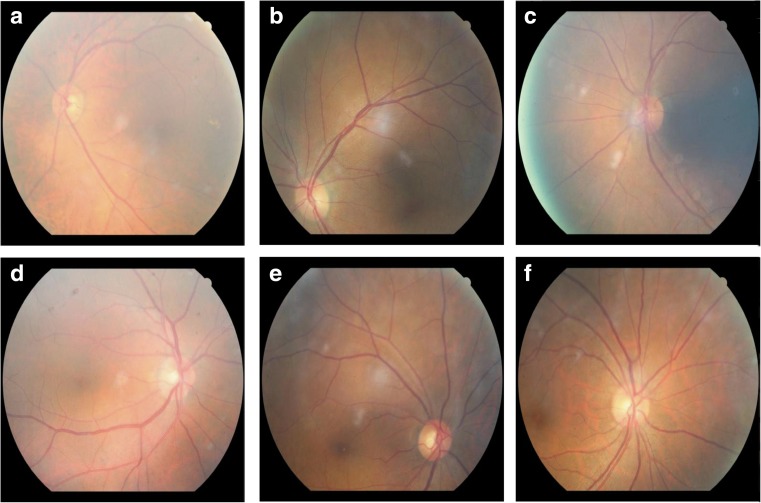
We used the retinal fundus image database of Seoul National University Bundang Hospital after removing all patient-specific information (e.g., patient identification number, name, date of birth, age, sex, study date, diagnosis, other clinical information). The images in the database were converted into Joint Photographic Experts Group (JPEG) format with randomly generated, laterality-indicative filenames. We included 25,911 retinal fundus images in the present study; 43.4% of these images were macula-centered images and the remaining 28.3% each were superior and nasal images. Figure 1 illustrates several examples of macular-centered, superior, and nasal images. This study was approved by the Institutional Review Board (IRB) of Seoul National University Bundang Hospital (IRB no. B-1508-312-107), and requirement of informed consent was waived from the IRB. The study complied with the guidelines of the Declaration of Helsinki.

Fig. 1.

Examples of fundus images in the Retinal Fundus Photo Database in SNU Bundang Hospital. Each column illustrates example images of center, superior, and nasal fundi, respectively. a–c correspond to ocular sinister (left) and d–f correspond to ocular dexter (right)

Pre-Processing

Before the training phase, every RGB channel of an input image was normalized to a z-score [5]. This ensures that classification results to be invariant of intensities and color contrasts of the images and therefore enables the model to make predictions solely based on the shape configurations of the fundi. The black background of the fundus images was excluded in normalization.

Model Architecture

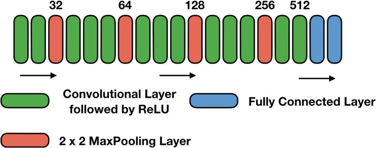
Our model consists of five blocks of convolutional layers of 3 × 3 kernels, 2 × 2 strides with a ReLU activation function, followed by two fully connected layers with a softmax activation function that has two nodes in the output layer (illustrated in Fig. 2).

Fig. 2.

Overview of our neural network architecture. Starting from 32 convolution filters, the number of filters increases by a factor of 2 after every max pooling layer (indicated by the numbers above the boxes). The first FC layer uses a ReLU activation function with 256 filters, followed by the second FC layer with a softmax activation function and two filters. The last layer is a softmax output with two nodes

Also, the cross-entropy loss function is used with L2 regularization for weights in the network, given by Eq. (1):

$$C\left(\widehat{y},y\right)=-\frac{1}{n}{\sum }_i\left[y_{i}log{\widehat{y}}_i+\left(1-y_i\right)log\left(1-{\widehat{y}}_i\right)\right]+\frac{\mathrm{\lambda }}{2n}{\sum }_k{w}_k^2$$ 1

where n denotes the number of samples in the training data, y_i is the output label (indicated by 0 or 1 in binary classification task), and ${\widehat{y}}_i$ is the output prediction for a sample image. Here, λ is set to be 0.0005, which was chosen by random search between 0.001 and 0.0001. We have also added L2 regularization for biases in a similar fashion to Eq. (1). Our model is implemented using Keras, an open-source neural network library written in Python, with Tensorflow backend. We have run the iterations for 100 epochs for training, which showed convergence of validation loss and set the keep-rate of all dropout layers to be 0.5 as widely used in the literature.

Guided Grad-Class Activation Mapping

Class Activation Mapping [6] (CAM) is useful in visualizing activation maps of features of interest, since convolutional layers are known to contain spatial information, and therefore can be treated as feature extractors. It can also be used as a debugging tool; it allows to judge if the model predictions are correct and reliable. However, CAM requires some adjustments to the existing model: removal of fully connected layers and retraining of the modified model. This modification might lead to a considerable loss in accuracy. For this reason, we employ Grad-CAM method, a generalization of CAM, which does not require any modifications nor retraining of the model.

The activation map for class c is obtained by first calculating the importance weights ${\alpha }_k^c$ via global average pooling:

$${\alpha }_k^c=\frac{1}{Z}\sum _i\sum _j\frac{\partial y^c}{\partial A_{\mathit{ij}}^k}$$

where Z is the normalizing constant, $A_{\mathit{ij}}^k$ denotes each pixel of the activation map A^k , and $w_k^c$ denotes the class feature weights.

Grad-CAM heatmap for class c, L^c, is simply a rectified, weighted combination of feature maps.

$$L^c=\mathit{\text{ReLU}}\left(\sum _k{\alpha }_k^c{A}^k\right)$$

In addition, guided backpropagation is used along with Grad-CAM, which is a slight variant of backpropagation method. It has been shown that guided Grad-CAM gives much clearer class-discriminative activation maps than CAM or Grad-CAM [7].

Dropout Uncertainty

A model confidence is not captured by standard deep learning tools and is often misinterpreted by the model prediction. It has been shown that uncertainty information can be obtained from the model predictions using dropout layers: by sampling from Bernoulli distribution of probability equal to keep rate at dropout layers. This is equivalent in practice to running several forward passes through the neural network and calculating the predictive variance. Formally, we calculate the empirical estimator for predictive mean by running T forward passes:

$$E\left[y\right]\approx \frac{1}{T}\sum _{i=1}^T{\widehat{y}}_i\left(x\right)$$

where x is the input vector and $\widehat{y}$ denotes the output vector of the prediction. The empirical estimator for predictive variance is given as follows:

$$\mathit{Var}\left[y\right]\approx {\tau }^{-1}{I}_D+\frac{1}{T}\sum _{i=1}^T{\widehat{y}}_i{\left(x\right)}^T{\widehat{y}}_i\left(x\right)-E{\left[y\right]}^{T}E\left[y\right]$$

where τ is the model precision (omitted) and I_D denotes the identity matrix. The variance information can be used to detect images for which the model is unsure of its predictions. The benefit of dropout Bayesian approximation method is that it allows to estimate the prediction uncertainties by simply collecting the results from existing neural network [8].

Experimental Setup

The dataset is randomly partitioned into training and validation sets of the ratio of 8 to 2, and we perform 5-fold cross-validation. By running the same number of epochs five times, we find the sample mean of resulting prediction probabilities. Also, we used Grad-CAM [7] technology to highlight regions that the network focuses on for the classification and dropout layers via Bayesian approximation [8] for estimation of uncertainty in predictions.

Results

Model Performance

We compared classification accuracy with VGG-16 [9] and AlexNet [4]. In both networks, only the number of nodes in the last softmax layer is changed to 2 and the networks are trained from the scratch with the same hyperparameters (weight decay, number of epochs, keep rate in dropout). Our model has achieved an accuracy of mean 98.9% with standard deviation of 0.11% (Table 1) in all types of images outperforming VGG-16 and performing similarly to AlexNet. Also, similar trends were observed when accuracy is measured separately for superior, nasal, and center images. Note that our model entails about a half as many parameters as AlexNet does but performs similarly.

Table 1.

Performance comparisons among our model, AlexNet, and VGG-16 architectures via 5-fold cross-validation

	Image type								No. of params
	Superior		Nasal		Center		All
	Mean	Standard deviation	Mean	Standard deviation	Mean	Standard deviation	Mean	Standard deviation
Our model	98.38%	0.77%	99.61%	0.10%	99.24%	0.30%	98.98%	0.11%	13,876,194
AlexNet	98.19%	0.44%	99.56%	0.01%	99.47%	0.21%	98.96%	0.08%	24,100,226
Vgg-16	97.94%	0.53%	99.47%	0.12%	99.47%	0.28%	98.50%	0.17%	89,954,626

Guided Grad-CAM Heatmaps

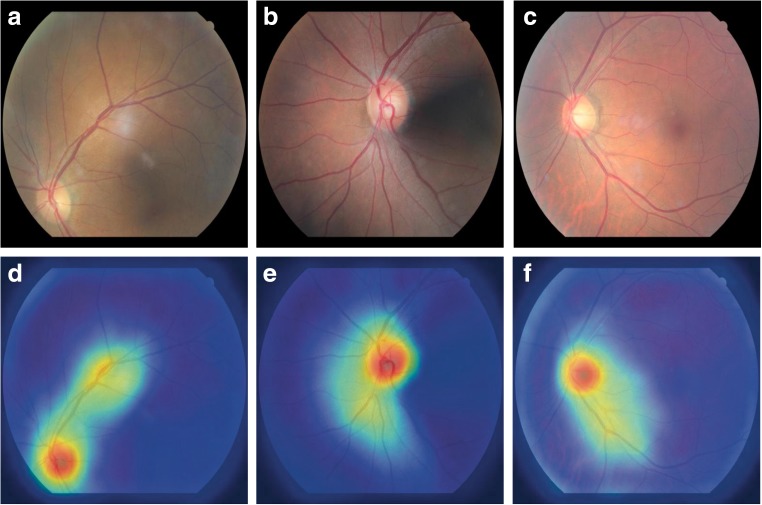
As illustrated in Fig. 3, we can generate evident and coherent activation maps for most images in the dataset using guided Grad-CAM visualization method. We observe dominant activations at optic discs and relatively lower activations along the retinal blood vessels. This corresponds to what human experts tend to see when classifying laterality of fundus images: the location of optic disc and the arrangements of blood vessels [10].

Fig. 3.

Guided Grad-CAM activation maps generated from superior, nasal, and center fundus images. a–c are original fundus images (superior, nasal, center) and d–f correspond to activation maps of superior, nasal, and center fundus, respectively. High activations are observed at the location of optic disc and the surrounding vasculature

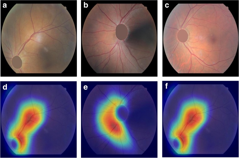
We further eliminate optic discs from fundus images and re-generate guided Grad-CAM heatmaps while maintaining the model. Since the model is trained with images of untouched optic discs, it is expected that the model could not recognize the disc. The occlusion of optic discs is done by performing segmentation with U-net [11] (trained using images in the DRION database [12]) and filling the pixels of the optic disc with the average value of the surrounding pixels. As shown in Fig. 4, when the optic disc is occluded, the activations are more widespread along retinal blood vessels, which is also interesting as clinicians would look at vessel branches around the disc when the disc is not fully visible. We also notice minimal activations at the occlusion region (i.e., the location of optic disc). This trend is consistent regardless of the macular centrality of the fundus images.

Fig. 4.

Guided Grad-CAM activation maps when the optic discs are occluded. a–c are fundus images of which the optic discs are occluded (superior, nasal, and center) and d–f correspond to activation maps of the fundus images. High activations are observed along the retinal blood vessels excluding the optic disc

We conclude that our model considers the information of optic disc as well as that of the neighboring retinal blood vessels for laterality classification of fundus images.

Prediction Uncertainties

Using the dropout Bayesian approximation method, we calculate uncertainty (i.e., sample variance) of every fundus image in the validation set through 50 forward passes through the network. We perform the Mann-Whitney U test to examine whether there is a statistically significant difference in uncertainties between groups of correctly and incorrectly classified images. Mann-Whitney U test is a non-parametric test which does not require samples to follow a known distribution, which is suitable to the purpose of our analysis. It turned out that the means of uncertainties of images from these two groups are significantly different from each other (p value < 0.0001). This result supports the claim that incorrectly classified images do have higher prediction uncertainties than correctly classified images. It has been observed that the means of the uncertainties in two groups differ by a magnitude of order of 2.

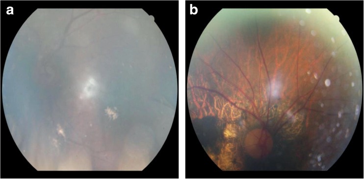
Figure 5 shows two direct examples of incorrectly classified fundus images. These images are not usable in practice for detection of fundus diseases or any other types of fundus examinations as they do not show the fundus in its entirety; for instance, optic disc and the retinal blood vessels are not clearly visible. The first image is extremely opaque, and the second image contains many black spots that substantially interfere with the image.

Fig. 5.

Two examples of incorrectly classified fundus images by our neural network

Discussion

Our convolutional neural network showed accuracy of 99%, which is comparable to the performance of clinicians as is the case for other deep learning systems for other image classification tasks. In fact, the classification of laterality is straightforward but mundane that clinicians do not favor to do. Also, there exists potential that human errors due to fatigues and mistakes in manipulation lead to wrong decisions. In that sense, the automated system would have practical benefits when deployed in clinics as the burdens of clinicians are reduced significantly.

Furthermore, it is also imperative for clinicians to understand how the decision is made from the automated system, since the results cannot be trusted otherwise. To resolve this issue, we visualized regions in the image that the neural network pays attention for the decision. We found that optic disc and the surrounding vessels are determinant regions in the images that decide the laterality. This is interesting because clinicians also look at the disc and vessels around it for making the decision.

With uncertainty analysis, it is possible to translate the degree of confidence in the decision from the neural network into a concrete number. Convolutional neural networks only do return prediction results, though it is also possible to approximate the uncertainty in the decision with the technical trick proposed recently. From our data, we discovered that misclassified images tend to have higher uncertainty than correctly classified images and misclassified images mainly consist of ungradable images. In fact, the ability to estimate uncertainty is also beneficial and critical in the clinical context as the system should refer to clinicians when unsure of its decision.

In conclusion, we expect that our model not only improves the efficiency of fundus laterality classification in clinics by delivering prompt and automatic predictions with high accuracy but also provides promising ways to interacting with an automated system for clinicians by presenting determinant regions for the decision and estimating uncertainty in the decision.

Funder/Sponsor

This study was supported by the Small Grant for Exploratory Research of the National Research Foundation of Korea (NRF), which is funded by the Ministry of Science, ICT, and Future Planning (NRF-2015R1D1A1A02062194). The funding organizations had no role in the design or conduct of this research.

Compliance with Ethical Standards

Conflict of Interest

The authors declare that they have no conflict of interest.

References

- 1.Jaya T, Dheeba J, Singh NA. Detection of hard exudates in colour fundus images using fuzzy support vector machine-based expert system. J Digit Imaging. 2015;28(6):761–768. doi: 10.1007/s10278-015-9793-5. [DOI] [PMC free article] [PubMed] [Google Scholar]
- 2.Oloumi F, Rangayyan RM, Ells AL. Computer-aided diagnosis of proliferative diabetic retinopathy via modeling of the major temporal arcade in retinal fundus images. J Digit Imaging. 2013;26(6):1124–1130. doi: 10.1007/s10278-013-9592-9. [DOI] [PMC free article] [PubMed] [Google Scholar]
- 3.Group, E.T.D.R.S.R Grading diabetic retinopathy from stereoscopic color fundus photographs--an extension of the modified Airlie house classification. ETDRS report number 10. Early treatment diabetic retinopathy study research group. Ophthalmology. 1991;98(5 Suppl):786–806. [PubMed] [Google Scholar]
- 4.Krizhevsky, A.a.S., Ilya and Hinton, Geoffrey E, Imagenet classification with deep convolutional neural networks, in Advances in Neural Information Processing Systems. 2012. p. 1097–1105.
- 5.Ulyanov, D.a.V., Andrea and Lempitsky, victor, Instance normalization: The missing ingredient for fast stylization. arXiv preprint arXiv:1607.08022, 2016.
- 6.Zhou, B.a.K., Aditya and Lapedriza, Agata and Oliva, Aude and Torralba, Antonio. Learning deep features for discriminative localization. in IEEE conference on computer vision and pattern recognition. 2016.
- 7.Selvaraju, R.R.a.C., Michael and Das, Abhishek and Vedantam, Ramakrishna and Parikh, Devi and Batra, Dhruv, Grad-CAM: Visual Explanations from Deep Networks via Gradient-based Localization. arXiv preprint arXiv:1610.02391, 2016.
- 8.Gal, Y.a.G., Zoubin. Dropout as a Bayesian approximation: Representing model uncertainty in deep learning. in International conference on machine learning. 2016.
- 9.Simonyan, K.a.Z., Andrew, Very deep convolutional networks for large-scale image recognition. arXiv preprint arXiv:1409.1556, 2014.
- 10.Schneiderman, H., The Funduscopic Examination, in Clinical Methods: The History, Physical, and Laboratory Examinations, rd, et al., Editors. 1990: Boston.
- 11.Ronneberger, O.a.F., Philipp and Brox, Thomas, U-net: Convolutional networks for biomedical image segmentation, in International Conference on Medical Image Computing and Computer-Assisted Intervention. 2015, Springer. p. 234–241.
- 12.Carmona EJ, Rincón M, García-Feijoó J, Martínez-de-la-Casa JM. Identification of the optic nerve head with genetic algorithms. Artif Intell Med. 2008;43(3):243–259. doi: 10.1016/j.artmed.2008.04.005. [DOI] [PubMed] [Google Scholar]