NeuralNetTools: Visualization and Analysis Tools for Neural Networks

Abstract

Supervised neural networks have been applied as a machine learning technique to identify and predict emergent patterns among multiple variables. A common criticism of these methods is the inability to characterize relationships among variables from a fitted model. Although several techniques have been proposed to “illuminate the black box”, they have not been made available in an open-source programming environment. This article describes the NeuralNetTools package that can be used for the interpretation of supervised neural network models created in R. Functions in the package can be used to visualize a model using a neural network interpretation diagram, evaluate variable importance by disaggregating the model weights, and perform a sensitivity analysis of the response variables to changes in the input variables. Methods are provided for objects from many of the common neural network packages in R, including caret, neuralnet, nnet, and RSNNS. The article provides a brief overview of the theoretical foundation of neural networks, a description of the package structure and functions, and an applied example to provide a context for model development with NeuralNetTools. Overall, the package provides a toolset for neural networks that complements existing quantitative techniques for data-intensive exploration.

1. Introduction

A common objective of data-intensive analysis is the synthesis of unstructured information to identify patterns or trends “born from the data” (Bell, Hey, and Szalay 2009; Kelling, Hochachka, Fink, Riedewald, Caruana, Ballard, and Hooker 2009; Michener and Jones 2012). Analysis is primarily focused on data exploration and prediction as compared to hypothesistesting using domain-specific methods for scientific exploration (Kell and Oliver 2003). Demand for quantitative toolsets to address challenges in data-rich environments has increased drastically with the advancement of techniques for rapid acquisition of data. Fields of research characterized by high-throughput data (e.g., bioinformatics; Saeys, Inza, and Larrañaga 2007) have a strong foundation in computationally-intensive methods of analysis, whereas disciplines that have historically been limited by data quantity (e.g., field ecology; Swanson, Kosmala, Lintott, Simpson, Smith, and Packer 2015) have also realized the importance of quantitative toolsets given the development of novel techniques to acquire information. Quantitative methods that facilitate inductive reasoning can serve a complementary role to conventional, hypothesis-driven approaches to scientific discovery (Kell and Oliver 2003).

Statistical methods that have been used to support data exploration are numerous (Jain, Duin, and Mao 2000; Recknagel 2006; Zuur, Ieno, and Elphick 2010). A common theme among data intensive methods is the use of machine-learning algorithms where the primary objective is to identify emergent patterns with minimal human intervention. Neural networks, in particular, are designed to mimic the neuronal structure of the human brain by “learning” inherent data structures through adaptive algorithms (Rumelhart, Hinton, and Williams 1986; Ripley 1996). Although the conceptual model was introduced several decades ago (McCulloch and Pitts 1943), neural networks have had a central role in emerging fields focused on data exploration. The most popular form of neural network is the feed-forward multilayer perceptron (MLP) trained using the backpropagation algorithm (Rumelhart et al. 1986). This model is typically used to predict the response of one or more variables given one to many explanatory variables. The hallmark feature of the MLP is the characterization of relationships using an arbitrary number of parameters (i.e., the hidden layer) that are chosen through iterative training with the backpropagation algorithm. Conceptually, the MLP is a hyper-parameterized non-linear model that can fit a smooth function to any dataset with minimal residual error (Hornik 1991).

An arbitrarily large number of parameters to fit a neural network provides obvious predictive advantages, but complicates the extraction of model information. Diagnostic information such as variable importance or model sensitivity are necessary aspects of exploratory data analysis that are not easily obtained from a neural network. As such, a common criticism is that neural networks are “black boxes” that offer minimal insight into relationships among variables (e.g., Paruelo and Tomasel 1997). Olden and Jackson (2002) provide a rebuttal to this concern by describing methods to extract information about variable relationships from neural networks. Many of these methods were previously described but not commonly used. For example, Olden and Jackson (2002) describe the neural interpretation diagram (NID) for plotting (Özesmi and Özesmi 1999), the Garson algorithm for variable importance (Garson 1991), and the profile method for sensitivity analysis (Lek, Delacoste, Baran, Dimopoulos, Lauga, and Aulagnier 1996). These quantitative tools “illuminate the black box” by disaggregating the network parameters to characterize relationships between variables that are described by the model. Although MLP neural networks were developed for prediction, methods described in Olden and Jackson (2002) leverage these models to describe data signals. Increasing the accessibility of these diagnostic tools will have value for exploratory data analysis and may also inform causal inference.

This article describes the NeuralNetTools package (Beck 2018) for R (R Core Team 2018) that was developed to better understand information obtained from the MLP neural network. Functions provided by the package are those described in Olden and Jackson (2002) but have not been previously available in an open-source programming environment. The reach of the package is extensive in that generic functions were developed for model objects from the most popular neural network packages available in R. The objectives of this article are to 1) provide an overview of the statistical foundation of the MLP network, 2) describe the theory and application of the main functions in the NeuralNetTools package, and 3) provide an applied example using neural networks and NeuralNetTools in data exploration. The current released package version is available from the Comprehensive R Archive Network (CRAN) at https://CRAN.R-project.org/package=NeuralNetTools, whereas the development version is maintained as a GitHub repository.

2. Theoretical foundation and existing R packages

The typical MLP network is composed of multiple layers that define the transfer of information between input and response layers. Information travels in one direction where a set of values for variables in the input layer propagates through one or more hidden layers to the final layer of the response variables. Hidden layers between the input and response layers are key components of a neural network that mediate the transfer of information. Just as the input and response layers are composed of variables or nodes, each hidden layer is composed of nodes with weighted connections that define the strength of information flow between layers. Bias layers connected to hidden and response layers may also be used that are analogous to intercept terms in a standard regression model.

Training a neural network model requires identifying the optimal weights that define the connections between the model layers. The optimal weights are those that minimize prediction error for a test dataset that is independent of the training dataset. Training is commonly achieved using the backpropagation algorithm described in Rumelhart et al. (1986). This algorithm identifies the optimal weighting scheme through an iterative process where weights are gradually changed through a forward- and backward-propagation process (Rumelhart et al. 1986; Lek and Guégan 2000). The algorithm begins by assigning an arbitrary weighting scheme to the connections in the network, followed by estimating the output in the response variable through the forward-propagation of information through the network, and finally calculating the difference between the predicted and actual value of the response. The weights are then changed through a backpropagation step that begins by changing weights in the output layer and then the remaining hidden layers. The process is repeated until the chosen error function is minimized, as in standard model-fitting techniques for regression (Cheng and Titterington 1994). A fitted MLP neural network can be represented as (Bishop 1995; Venables and Ripley 2002):

$$y_k=f_o\left(\sum _h{w}_{hk}{f}_h\left(\sum _i{w}_{ih}{x}_i\right)\right),$$ (1)

where the estimated value of the response variable yk is a sum of products between the respective weights w for i input variables x and h hidden nodes, mediated by the activation functions fh and fo for each hidden and output node.

Methods in NeuralNetTools were written for several R packages that can be used to create MLP neural networks: neuralnet (Fritsch and Guenther 2016), nnet (Venables and Ripley 2002), and RSNNS (Bergmeir and Benítez 2012). Limited methods were also developed for neural network objects created with the train function from the caret package (Kuhn 2008). Additional R packages that can create MLP neural networks include AMORE that implements the “TAO-robust backpropagation algorithm” for model fitting (Castejón Limas, Ordieres Meré, González Marcos, de Pisón Ascacibar, Pernía Espinoza, Alba Elías, and Perez Ramos 2014), FCNN4R that provides an R interface to the FCNN C++ library (Klima 2016), monmlp for networks with partial monotonicity constraints (Cannon 2017), and qrnn for quantile regression neural networks (Cannon 2011). At the time of writing, the CRAN download logs (Csardi 2015) showed that the R packages with methods in NeuralNetTools included 95% of all downloads for the available MLP packages, with nnet accounting for over 78%. As such, methods have not been included in NeuralNetTools for the remaining packages, although further development of NeuralNetTools could include additional methods based on popularity. Methods for each function are currently available for ‘mlp’ (RSNNS), ‘nn’ (neuralnet), ‘nnet’ (nnet), and ‘train’ (caret; only if the object also inherits from the ‘nnet’ class) objects. Additional default methods or methods for class ‘numeric’ are available for some of the generic functions.

3. Package structure

The stable release of NeuralNetTools can be installed from CRAN and loaded as follows:

R> install.packages(“NeuralNetTools”)
R> library(“NeuralNetTools”)

NeuralNetTools includes four main functions that were developed following similar techniques in Olden and Jackson (2002) and references therein. The functions include plotnet to plot a neural network interpretation diagram, garson and olden to evaluate variable importance, and lekprofile for a sensitivity analysis of neural network response to input variables. Most of the functions require the extraction of model weights in a common format for the neural network object classes in R. The neuralweights function can be used to retrieve model weights for any of the model classes described above. A two-element list is returned with the first element describing the structure of the network (number of nodes in the input, hidden, and output layers) and the second element as a named list of model weights. The function is used internally within the main functions but may also be useful for comparing networks of different classes.

A common approach for data pre-processing is to normalize the input variables and to standardize the response variables (Lek and Guégan 2000; Olden and Jackson 2002). A sample dataset that follows this format is included with NeuralNetTools. The neuraldat dataset is a simple data.frame with 2000 rows of observations and five columns for two response variables (Y1 and Y2) and three input variables (X1, X2, and X3). The input variables are random observations from a standard normal distribution and the response variables are linear combinations of the input variables with additional random components. The response variables are also scaled from zero to one. Variables in additional datasets can be pre-processed to this common format using the scale function from base to center and scale input variables (i.e., z-scores) and the rescale function from scales to scale response variables from zero to one. The examples below use three models created from the neuraldat dataset and include ‘mlp’ (RSNNS), ‘nn’ (RSNNS), and ‘nnet’ (nnet) objects.

R> set.seed(123)
R> library(“RSNNS”)
R> x <- neuraldat[, c(“X1”, “X2”, “X3”)]
R> y <- neuraldat[, “Y1”]
R> mod1 <- mlp(x, y, size = 5)
R> library(“neuralnet”)
R> mod2 <- neuralnet(Y1 ~ X1 + X2 + X3, data = neuraldat, hidden = 5)
R> library(“nnet”)
R> mod3 <- nnet(Y1 ~ X1 + X2 + X3, data = neuraldat, size = 5)

3.1. Visualizing neural networks

Existing plot functions in R to view neural networks are minimal. Such tools have practical use for visualizing network architecture and connections between layers that mediate variable importance. To our knowledge, only the neuralnet and FCNN4R packages provide plotting methods for MLP networks in R. Although useful for viewing the basic structure, the output is minimal and does not include extensive options for customization.

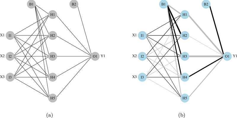
The plotnet function in NeuralNetTools plots a neural interpretation diagram (NID; Özesmi and Özesmi 1999) and includes several options to customize aesthetics. A NID is a modification of the standard conceptual illustration of the MLP network that changes the thickness and color of the weight connections based on magnitude and sign, respectively. Positive weights between layers are shown as black lines and negative weights as gray lines. Line thickness is proportional to the absolute magnitude of each weight (Figure 1).

Figure 1:

Examples from the plotnet function showing neural networks as a standard graphic (1a) and using the neural interpretation diagram (1b). Labels outside of the nodes represent variable names and labels within the nodes indicate the layer and node (I: input, H: hidden, O: output, B: bias).

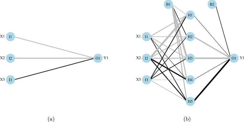
A primary and skip layer network can also be plotted for ‘nnet’ models with a skip layer connection (Figure 2). Models with skip layers include additional connections from the input to output layers that bypass the hidden layer (Ripley 1996). The default behavior of plotnet is to plot the primary network, whereas the skip layer can be viewed separately with skip = TRUE. If nid = TRUE, the line widths for both the primary and skip layer plots are relative to all weights. Plotting a network with only a skip layer (i.e., no hidden layer, size = 0 in nnet) will include bias connections to the output layer, whereas these are included only in the primary plot if size is greater than zero.

Figure 2:

Examples from the plotnet function showing a neural network with a separate skip layer between the input and output layers. The skip layer (2a) and primary neural network (2b) can be viewed separately with plotnet by using skip = TRUE or skip = FALSE.

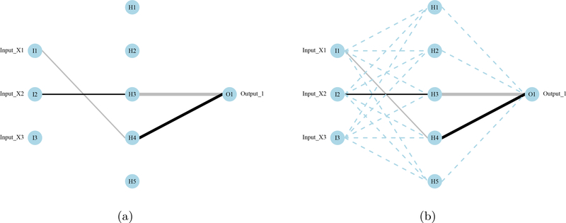
The RSNNS package provides algorithms to prune connections or nodes in a neural network (Bergmeir and Benítez 2012). This approach can remove connection weights between layers or input nodes that do not contribute to the predictive performance of the network. In addition to visualizing connections in the network that are not important, connections that are pruned can be removed in successive model fitting. This reduces the number of free parameters (weights) that are estimated by the model optimization algorithm, increasing the likelihood of convergence to an estimable numeric solution for the remaining connection weights that minimizes prediction error (i.e., model identifiability; Ellenius and Groth 2000). Algorithms in RSNNS for weight pruning include magnitude-based pruning, optimal brain damage, and optimal brain surgeon, whereas algorithms for node pruning include skeletonization and the non-contributing units method (Zell, Mamier, Vogt, Mache, Hübner, Döring, Herrmann, Soyez, Schmalzl, Sommer, Hatzigeorgiou, Posselt, Schreiner, Kett, Clemente, Wieland, and Gatter 1998). The plotnet function can plot a pruned neural network, with options to omit or display the pruned connections (Figure 3).

Figure 3:

A pruned neural network from RSNNS (Bergmeir and Benítez 2012) using the “optimal brain surgeon” algorithm described in Zell et al. (1998). The default plotting behavior of plotnet is to omit pruned connections (3a), whereas they can be viewed as dashed lines by including the prune_col argument (3b).

R> pruneFuncParams <- list(max_pr_error_increase = 10.0,
+ pr_accepted_error = 1.0, no_of_pr_retrain_cycles = 1000,
+ min_error_to_stop = 0.01, init_matrix_value = 1e-6,
+ input_pruning = TRUE, hidden_pruning = TRUE)
R> mod <- mlp(x, y, size = 5, pruneFunc = “OptimalBrainSurgeon”,
+ pruneFuncParams = pruneFuncParams)
R> plotnet(mod, rel_rsc = c(3, 8))
R> plotnet(mod, prune_col = “lightblue”, rel_rsc = c(3, 8))

Note that the pruned network obtained with RSNNS and thus this plot might vary depending on the platform used.

3.2. Evaluating variable importance

The primary benefit of visualizing a NID with plotnet is the ability to evaluate network architecture and the variation in connections between the layers. Although useful as a general tool, the NID can be difficult to interpret given the amount of weighted connections in most networks. Alternative methods to quantitatively describe a neural network deconstruct the model weights to determine variable importance, whereas similar information can only be qualitatively inferred from plotnet. Two algorithms for evaluating variable importance are available in NeuralNetTools: Garson’s algorithm for relative importance (Garson 1991; Goh 1995) and Olden’s connection weights algorithm (Olden, Joy, and Death 2004).

Garson’s algorithm was originally described by Garson (1991) and further modified by Goh (1995). The garson function is an implementation of the method described in the appendix of Goh (1995) that identifies the relative importance of each variable as an absolute magnitude. For each input node, all weights connecting an input through the hidden layer to the response variable are identified to return a list of all weights specific to each input variable. Summed products of the connections for each input node are then scaled relative to all other inputs. A value for each input node indicates relative importance as the absolute magnitude from zero to one. The method is limited in that the direction of the response cannot be determined and only neural networks with one hidden layer and one output node can be evaluated. The olden function is a more flexible approach to evaluate variable importance using the connection weights algorithm (Olden et al. 2004). This method calculates importance as the summed product of the raw input-hidden and hidden-output connection weights between each input and output node. An advantage is the relative contributions of each connection weight are maintained in both magnitude and sign. For example, connection weights that change sign (e.g., positive to negative) between the input-hidden to hidden-output layers would have a canceling effect, whereas garson may provide different results based on the absolute magnitude. An additional advantage is that the olden function can evaluate neural networks with multiple hidden layers and response variables. The importance values assigned to each variable are also in units based on the summed product of the connection weights, whereas garson returns importance scaled from 0 to 1.

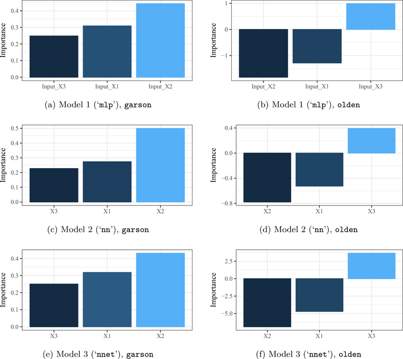
Both functions have similar implementations and require only a model object as input. The default output is a ggplot2 bar plot (i.e., geom_bar; Wickham 2009) that shows the relative importance of each input variable in the model (Figure 4). The plot aesthetics are based on internal code that can be changed using conventional syntax for ggplot2 applied to the output object. The importance values can also be returned as a data.frame if bar_plot = FALSE. Variable importance shown in Figure 4 is estimated for each model using:

Figure 4:

Variable importance for three models using Garson’s algorithm for relative importance (garson, Figures 4a, 4c and 4e; Garson 1991; Goh 1995) and Olden’s connection weights algorithm (olden, Figures 4b, 4d and 4f; Olden et al. 2004). Garson’s algorithm shows importance as absolute values from 0–1, whereas Olden’s algorithm preserves sign and magnitude. Importance values for Olden’s algorithm are from the summed product of model weights and are not rescaled.

R> garson(mod1)
R> olden(mod1)
R> garson(mod2)
R> olden(mod2)
R> garson(mod3)
R> olden(mod3)

3.3. Sensitivity analysis

An alternative approach to evaluate variable relationships in a neural network is the Lek profile method (Lek et al. 1996; Gevrey, Dimopoulos, and Lek 2003). The profile method differs fundamentally from the variable importance algorithms by evaluating the behavior of response variables across different values of the input variables. The method is generic and can be extended to any statistical model in R with a predict method. However, it is one of few methods used to evaluate sensitivity in neural networks.

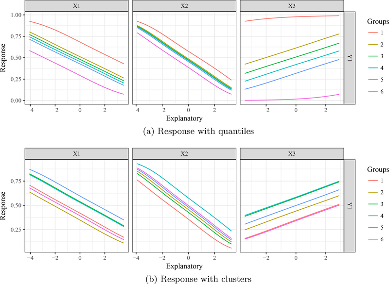
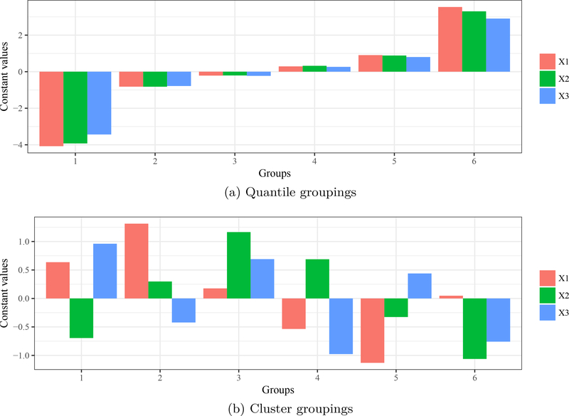
The lekprofile function evaluates the effects of input variables by returning a plot of model predictions across the range of values for each variable. The remaining explanatory variables are held constant when evaluating the effects of each input variable. The lekprofile function provides two options for setting constant values of unevaluated explanatory variables. The first option follows the original profile method by holding unevaluated variables at different quantiles (e.g., minimum, 20th percentile, maximum; Figures 5a and 6a). This is implemented by creating a matrix where the number of rows is the number of observations in the original dataset and the number of columns is the number of explanatory variables. All explanatory variables are held constant (e.g., at the median) while the variable of interest is sequenced from its minimum to maximum. This matrix is then used to predict values of the response variable from a fitted model object. This is repeated for each explanatory variable to obtain all response curves. Constant values are set in lekprofile by passing one or more values in the range 0–1 to the group_vals argument. The default holds variables at the minimum, 20th, 40th, 60th, 80th, and maximum percentiles (i.e., group_vals = c(0, 0.2, 0.4, 0.6, 0.8, 1)).

Figure 5:

Sensitivity analysis of a neural network using the Lek profile method to evaluate the effects of explanatory variables. Figure 5a groups unevaluated explanatory variables at quantiles (minimum, 20th, 40th, 60th, 80th, and maximum percentiles) and Figure 5b groups by cluster means (six groups). Values at which explanatory variables are held constant for each group are shown in Figures 6a and 6b.

Figure 6:

Bar plots for values of unevaluated explanatory variables in each group in Figures 5a and 5b. Figure 6a shows default quantile groupings set at the minimum, 20th, 40th, 60th, 80th, and maximum percentiles. For example, variables are held at negative values for group 1 (i.e., stacked bars with negative heights) for the minimum value, whereas group 6 holds variables at their maximum (largest positive heights). Figure 6b shows the cluster centers for each variable in each group. Groups in Figure 6b are random because the input variables are from a standard normal distribution.

A second implementation of lekprofile is to group the unevaluated explanatory variables by natural groupings defined by the data. Covariance among predictors may present unlikely scenarios if all unevaluated variables are held at the same level (e.g., high values for one variable may be unlikely with high values for a second variable). The second option holds unevaluated variables at means defined by natural clusters in the data (Figures 5b and 6b). Clusters are identified using k-means clustering (kmeans from the base package stats; Hartigan and Wong 1979) of the input variables if the argument passed to group_vals is an integer greater than one. The centers (means) of the clusters are then used as constants for the unevaluated variables. Beck, Wilson, Vondracek, and Hatch (2014) provide an example of the clustering method for lekprofile by evaluating response of a lake health index to different explanatory variables. Lake clusters were identified given covariance among variables, such that holding explanatory variables at values defined by clusters created more interpretable response curves. Both methods return similar plots, with additional options to visualize the groupings for unevaluated explanatory variables (Figure 6). For the latter case, group_show = TRUE will return a stacked bar plot for each group with heights within each bar proportional to the constant values. Sensitivity profiles were created using the standard approach based on quantiles and using the alternative clustering method (Figure 5), including bar plots of the relative values for unevaluated explanatory variables (Figure 6).

R> lekprofile(mod3)
R> lekprofile(mod3, group_show = TRUE)
R> lekprofile(mod3, group_vals = 6)
R> lekprofile(mod3, group_vals = 6, group_show = TRUE)

4. Applied example

Although NeuralnetTools provides several methods to extract information from a fitted neural network, it does not provide explicit guidance for developing the initial model. A potentially more challenging aspect of using MLP neural networks is understanding the effects of network architecture on model performance, appropriate use of training and validation datasets, and implications for the bias-variance tradeoff with model over- or under-fitting (Maier and Dandy 2000). A detailed discussion of these issues is beyond the scope of this paper, although an example application is presented below to emphasize the importance of these considerations. The models presented above, including the neuraldat dataset, are contrived examples to illustrate use of the NeuralNetTools package and they do not demonstrate a comprehensive or practical application of model development. In general, the following should be considered during initial development (Ripley 1996; Lek and Guégan 2000; Maier and Dandy 2000):

• Initial data pre-processing to normalize inputs, standardize response, and assess influence of outliers.

• Network architecture including number of hidden layers, number of nodes in each hidden layer, inclusion of bias or skip layers, and pruning weights or inputs.

• Separating data into training and test datasets, e.g., 2:1, 3:1, leave-one-out, etc.

• Initial starting weights for the backpropagation algorithm.

• Criteria for stopping model training, e.g., error convergence tolerance, maximum number of iterations, minimum error on test dataset, etc.

A dataset from nycflights13 (Wickham 2017) is used to demonstrate (1) the use of the functions in NeuralNetTools to gain additional insight into relationships among variables, and (2) the effects of training conditions on model conclusions. This dataset provides information on all flights departing New York City (i.e., JFK, LGA, or EWR) in 2013. The example uses all flights from the UA carrier in the month of December to identify variables that potentially influence arrival delays (arr_delay, minutes) at the destination airport. Factors potentially related to delays are selected from the dataset and include departure delay (dep_delay, minutes), departure time (dep_time, hours, minutes), arrival time (arr_time, hours, minutes), travel time between destinations (air_time, minutes), and distance flown (distance, miles). First, the appropriate month and airline carrier are selected, all explanatory variables are scaled and centered, and the response variable is scaled to 0–1.

R> library(“nycflights13”)
R> library(“dplyr”)
R> tomod <- filter(flights, month == 12 & carrier == “UA”) %>%
+ select(arr_delay, dep_delay, dep_time, arr_time, air_time,
+ distance) %>% mutate_each(funs(scale), -arr_delay) %>%
+ mutate_each(funs(as.numeric), -arr_delay) %>%
+ mutate(arr_delay = scales::rescale(arr_delay, to = c(0, 1))) %>%
+ data.frame

Then, a standard MLP with five hidden nodes was created with the nnet package to model the effects of selected variables on arrival delays. The entire dataset is used for the example but separate training and validation datasets should be used in practice.

R> library(“nnet”)
R> mod <- nnet(arr_delay ~., size = 5, linout = TRUE, data = tomod,
+ trace = FALSE)

The default output is limited to structural information about the model and methods for model predictions (see str(mod) and ?predict.nnet). Using functions from NeuralNetTools, a more comprehensive understanding of the relationships between the variables is illustrated.

R> plotnet(mod)
R> garson(mod)
R> olden(mod)
R> lekprofile(mod, group_vals = 5)
R> lekprofile(mod, group_vals = 5, group_show = TRUE)

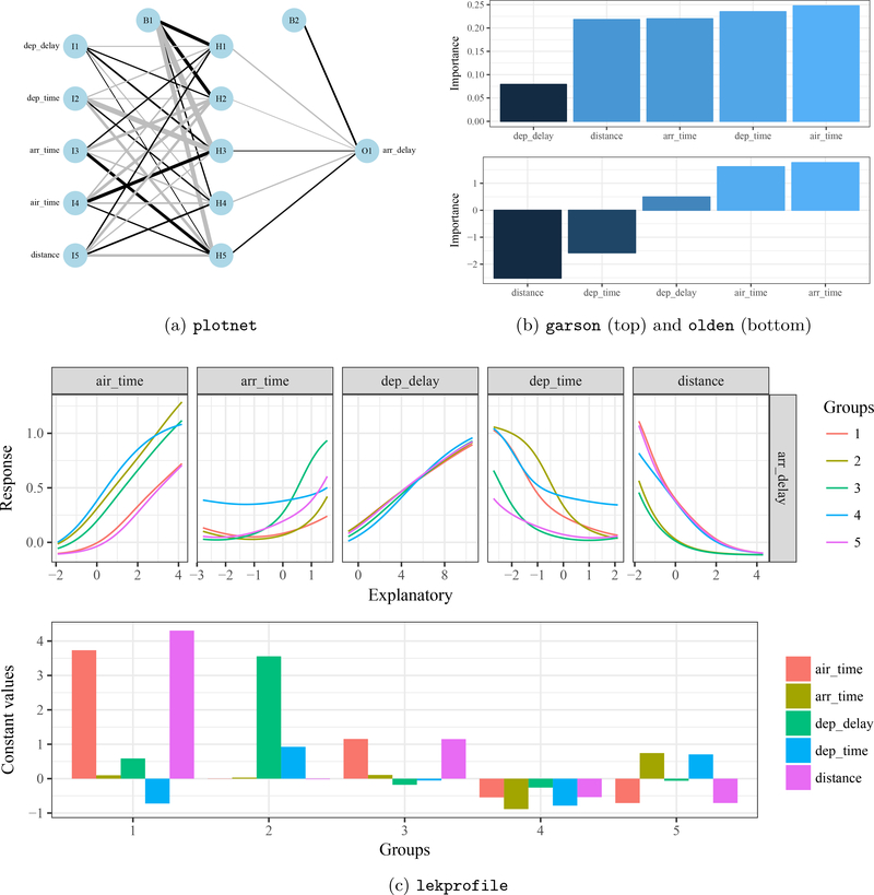
Figure 7 shows the information about arrival delays that can be obtained with the functions in NeuralNetTools. The NID (7a) shows the model structure and can be used as a general characterization of the relationships between variables. For example, most of the connection weights from input nodes I2 and I5 are strongly negative (gray), suggesting that departure time and distance traveled has an opposing relationship with arrival delays. Similarly, large positive weights are observed for I3 and I4, suggesting arrival time and time in the air are positively associated with arrival delays. However, interpreting individual connection weights between layers is challenging. Figures 7b and 7c provide more quantitative descriptions using information from both the NID and model predictions. Figure 7b shows variable importance using the garson and olden algorithms. The garson function suggests time between destinations (air_time) has the strongest relationship with arrival delays, similar to a strong positive association shown with the olden method. However, the garson function shows arrival time (arr_time) as the third most important variable for arrival delays, whereas this is ranked highest by the olden function. Similar discrepancies between the two methods are observed for other variables, which are explained below. Finally, results from the lekprofile function (Figure 7c) confirm those in Figure 7b, with the addition of non-linear responses that vary by different groupings of the data. Values for each variable in the different unevaluated groups (based on clustering) show that there were no obvious patterns between groups, with the exception being group one that generally had longer times in the air and greater distance travelled.

Figure 7:

Results from a simple MLP model of arrival delay for December airline flights versus departure delay (dep_delay), departure time (dep_time), arrival time (arr_time), travel time between destinations (air_time), and distance flown (distance). The three plots show the NID from plotnet (7a), variable importance with garson and olden (7b), and sensitivity analysis with variable groupings from lekprofile (7c). Interpretations are provided in the text.

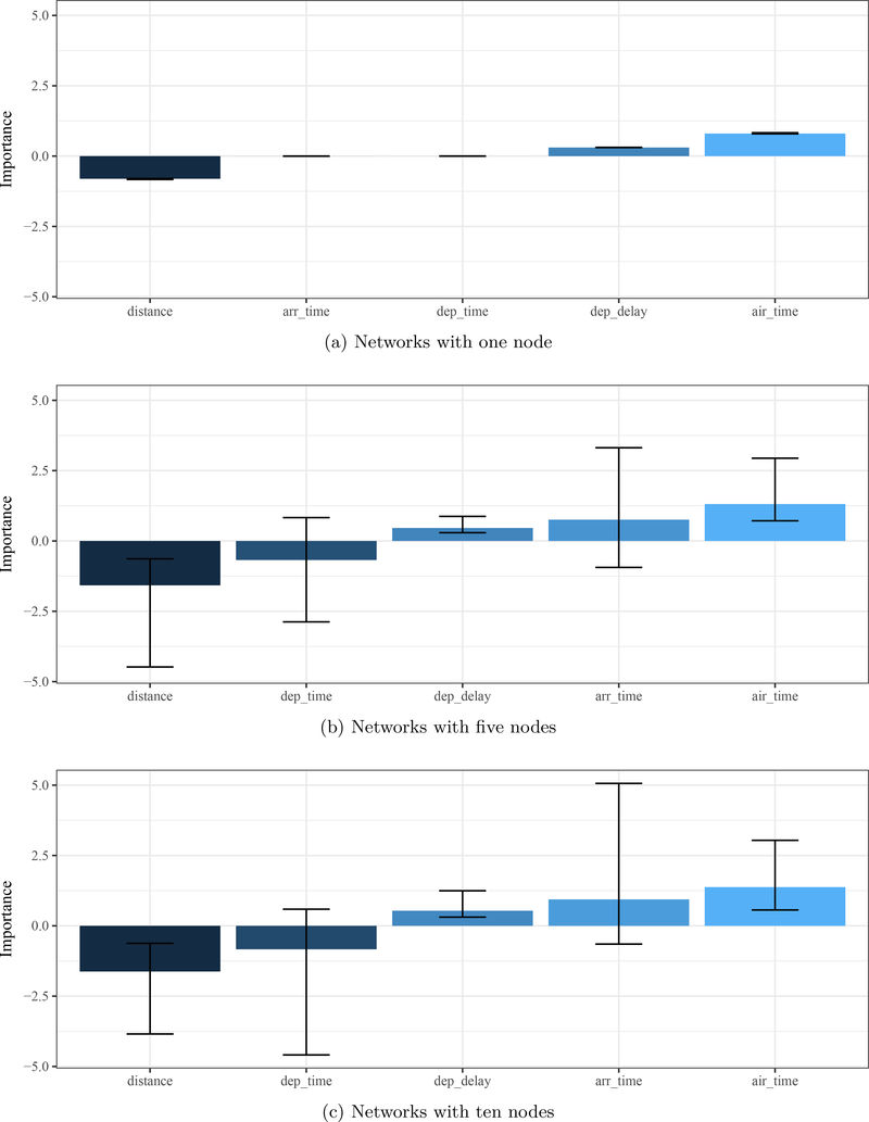
A second analysis is needed to show the effects of network architecture and initial starting weights on uncertainty in estimates of variable importance. Models with one, five, or ten hidden nodes and 100 separate models for each node level are created. Each model has a random set of starting weights for the first training iteration. Importance estimates using olden are saved for each model and combined in a single plot to show overall variable importance as the median and 5th/95th percentiles from the 100 models for each node level.

Several conclusions from Figure 8 provide further information to interpret the trends in Figure 7. First, consistent relationships can be identified such that delays in arrival time are negatively related to distance and positively related to departure delays and air time. That is, flights arrived later than their scheduled time if flight time was long or if their departure was delayed, whereas flights arrived earlier than scheduled for longer distances. No conclusions can be made for the other variables because the bounds of uncertainty include zero. Second, the range of importance estimates varies between the models (i.e., one node varies between ±1 and the others between ±3). This suggests that the relative importance estimates only have relevance within each model, whereas only the rankings (e.g., least, most important) can be compared between models. Third and most important, the level of uncertainty for specific variables can be large between model fits for the same architecture. This suggests that a single model can provide misleading information and therefore several models may be required to decrease uncertainty. Additional considerations described above (e.g., criteria for stopping training, use of training and test datasets) can also affect the interpretation of model information and should be considered equally during model development.

Figure 8:

Uncertainty in variable importance estimates for three neural networks to evaluate factors related to arrival delays for flights departing New York City. Three model types with one, five, and ten nodes were evaluated with 100 models with different starting weights for each type.

5. Conclusions

The NeuralNetTools package provides a simple approach to improve the quality of information obtained from a feed-forward MLP neural network. Functions can be used to visualize a neural network using a neural interpretation diagram (plotnet), evaluate variable importance (garson, olden), and conduct a sensitivity analysis (lekprofile). Although visualizing a neural network with plotnet is impractical for large models, the remaining functions can simplify model complexity to identify important relationships between variables. Methods are available for the most frequently used CRAN packages that can create neural networks (caret, neuralnet, nnet, RSNNS), whereas additional methods could be added based on popularity of the remaining packages (AMORE, FCNN4R, monmlp, qrnn).

A primary objective of the package is to address the concern that supervised neural networks are “black boxes” that provide no information about underlying relationships between variables (Paruelo and Tomasel 1997; Olden and Jackson 2002). Although neural networks are considered relatively complex statistical models, the theoretical foundation has many parallels with simpler statistical techniques that provide for evaluation of variable importance (Cheng and Titterington 1994). Moreover, the model fitting process minimizes error using a standard objective function such that conventional techniques to evaluate model sensitivity or performance (e.g., cross-validation) can be used with neural networks. As such, functions in NeuralNetTools can facilitate the selection of the optimal network architecture or can be used for post-hoc assessment.

Another important issue is determining when and how to apply neural networks given availability of alternative methods of analysis. The popularity of the MLP neural network is partly to blame for the generalizations and misperceptions about their benefits as modeling tools (Burke and Ignizio 1997). Perhaps an overstatement, the neural component is commonly advertised as a mathematical representation of the network of synaptic impulses in the human brain. Additionally, several examples have shown that the MLP network may provide comparable predictive performance as similar statistical methods (Feng and Wang 2002; Razi and Athappilly 2005; Beck et al. 2014). A neural network should be considered a tool in the larger toolbox of data-intensive methods that should be used after examination of the tradeoffs between techniques, with particular emphasis on the specific needs of a dataset or research question. Considerations for choosing a method may include power given the sample size, expected linear or non-linear interactions between variables, distributional forms of the response, and other relevant considerations of exploratory data analysis (Zuur et al. 2010). NeuralNetTools provides analysis tools that can inform evaluation and selection from among several alternative methods for exploratory data analysis.

References

- Beck M (2018). NeuralNetTools: Visualization and Analysis Tools for Neural Networks. R package version 1.5.2, URL https://CRAN.R-project.org/package=NeuralNetTools. [DOI] [PMC free article] [PubMed]
- Beck MW, Wilson BN, Vondracek B, Hatch LK (2014). “Application of Neural Networks to Quantify the Utility of Indices of Biotic Integrity for Biological Monitoring.” Ecological Indicators, 45, 195–208. doi:10.1016/j.ecolind.2014.04.002. [Google Scholar]
- Bell G, Hey T, Szalay A (2009). “Beyond the Data Deluge.” Science, 323(5919), 1297–1298. doi:10.1126/science.1170411. [DOI] [PubMed] [Google Scholar]
- Bergmeir C, Benítez JM (2012). “Neural Networks in R Using the Stuttgart Neural Network Simulator: RSNNS.” Journal of Statistical Software, 46(7), 1–26. doi:10.18637/jss.v046.i07.22837731 [Google Scholar]
- Bishop CM (1995). Neuronal Networks for Pattern Recognition. Carendon Press, Oxford. [Google Scholar]
- Burke L, Ignizio JP (1997). “A Practical Overview of Neural Networks.” Journal of Intelligent Manufacturing, 8(3), 157–165. doi:10.1023/a:1018513006083. [Google Scholar]
- Cannon AJ (2011). “Quantile Regression Neural Networks: Implementation in R and Application to Precipitation Downscaling.” Computers & Geosciences, 37(9), 1277–1284. doi: 10.1016/j.cageo.2010.07.005. [Google Scholar]
- Cannon AJ (2017). monmlp: Monotone Multi-Layer Perceptron Neural Network. R package version 1.1.5, URL https://CRAN.R-project.org/package=monmlp.
- Castejón Limas M, Ordieres Meré JB, González Marcos A, de Pisón Ascacibar FJM, Pernía Espinoza AV, Alba Elías F, Perez Ramos JM (2014). AMORE: A MORE Flexible Neural Network Package. R package version 0.2–15, URL https://CRAN.R-project.org/package=AMORE.
- Cheng B, Titterington DM (1994). “Neural Networks: A Review from a Statistical Perspective.” Statistical Science, 9(1), 2–30. doi:10.1214/ss/1177010638. [Google Scholar]
- Csardi G (2015). cranlogs: Download Logs from the RStudio CRAN Mirror. R package version 2.1.0, URL https://CRAN.R-project.org/package=cranlogs.
- Ellenius J, Groth T (2000). “Methods for Selection of Adequate Neural Network Structures with Application to Early Assessment of Chest Pain Patients by Biochemical Monitoring.” International Journal of Medical Informatics, 57(2–3), 181–202. doi: 10.1016/s1386-5056(00)00065-4. [DOI] [PubMed] [Google Scholar]
- Feng CX, Wang X (2002). “Digitizing Uncertainty Modeling for Reverse Engineering Applications: Regression Versus Neural Networks.” Journal of Intelligent Manufacturing, 13(3), 189–199. doi:10.1023/a:1015734805987. [Google Scholar]
- Fritsch S, Guenther F (2016). neuralnet: Training of Neural Networks. R package version 1.33, URL https://CRAN.R-project.org/package=neuralnet.
- Garson GD (1991). “Interpreting Neural Network Connection Weights.” Artificial Intelligence Expert, 6(4), 46–51. [Google Scholar]
- Gevrey M, Dimopoulos I, Lek S (2003). “Review and Comparison of Methods to Study the Contribution of Variables in Artificial Neural Network Models.” Ecological Modelling, 160(3), 249–264. doi:10.1016/s0304-3800(02)00257-0. [Google Scholar]
- Goh ATC (1995). “Back-Propagation Neural Networks for Modeling Complex Systems.” Artificial Intelligence in Engineering, 9(3), 143–151. doi:10.1016/0954-1810(94)00011-s. [Google Scholar]
- Hartigan JA, Wong MA (1979). “Algorithm AS 136: A K-Means Clustering Algorithm. Journal of the Royal Statistical Society C, 28(1), 100–108. doi:10.2307/2346830. [Google Scholar]
- Hornik K (1991). “Approximation Capabilities of Multilayer Feedforward Networks.” Neural Networks, 4(2), 251–257. doi:10.1016/0893-6080(91)90009-t. [Google Scholar]
- Jain AK, Duin RPW, Mao JC (2000). “Statistical Pattern Recognition: A Review.” IEEE Transactions on Pattern Analysis and Machine Intelligence, 22(1), 4–37. doi:10.1109/34.824819. [Google Scholar]
- Kell DB, Oliver SG (2003). “Here Is the Evidence, Now What Is the Hypothesis? The Complementary Roles of Inductive and Hypothesis-Driven Science in the Post-Genomic Era.” BioEssays, 26(1), 99–105. doi:10.1002/bies.10385. [DOI] [PubMed] [Google Scholar]
- Kelling S, Hochachka WM, Fink D, Riedewald M, Caruana R, Ballard G, Hooker G (2009). “Data-Intensive Science: A New Paradigm for Biodiversity Studies.” BioScience, 59(7), 613–620. doi:10.1525/bio.2009.59.7.12. [Google Scholar]
- Klima G (2016). FCNN4R: Fast Compressed Neural Networks for R. R package version 0.6.2, URL https://CRAN.R-project.org/package=FCNN4R.
- Kuhn M (2008). “Building Predictive Models in R Using the caret Package.” Journal of Statistical Software, 28(5), 1–26. doi:10.18637/jss.v028.i05.27774042 [Google Scholar]
- Lek S, Delacoste M, Baran P, Dimopoulos I, Lauga J, Aulagnier S (1996). “Application of Neural Networks to Modelling Nonlinear Relationships in Ecology.” Ecological Modelling, 90(1), 39–52. doi:10.1016/0304-3800(95)00142-5. [Google Scholar]
- Lek S, Guégan JF (2000). Artificial Neuronal Networks: Application to Ecology and Evolution. Springer-Verlag, Berlin. doi:10.1007/978-3-642-57030-8. [Google Scholar]
- Maier HR, Dandy GC (2000). “Neural Networks for the Prediction and Forecasting of Water Resources Variables: A Review of Modelling Issues and Applications.” Environmental Modelling and Software, 15(1), 101–124. doi:10.1016/s1364-8152(99)00007-9. [Google Scholar]
- McCulloch WS, Pitts W (1943). “A Logical Calculus of the Ideas Imminent in Nervous Activity.” Bulletin of Mathematical Biophysics, 5(4), 115–133. doi:10.1007/bf02478259. [PubMed] [Google Scholar]
- Michener WK, Jones MB (2012). “Ecoinformatics: Supporting Ecology as a Data-Intensive Science.” Trends in Ecology and Evolution, 27(2), 85–93. doi:10.1016/j.tree.2011.11.016. [DOI] [PubMed] [Google Scholar]
- Olden JD, Jackson DA (2002). “Illuminating the “Black Box”: A Randomization Approach for Understanding Variable Contributions in Artifical Neural Networks.” Ecological Modelling, 154(1–2), 135–150. doi:10.1016/s0304-3800(02)00064-9. [Google Scholar]
- Olden JD, Joy MK, Death RG (2004). “An Accurate Comparison of Methods for Quantifying Variable Importance in Artificial Neural Networks Using Simulated Data.” Ecological Modelling, 178(3–4), 389–397. doi:10.1016/j.ecolmodel.2004.03.013. [Google Scholar]
- Özesmi SL, Özesmi U (1999). “An Artificial Neural Network Approach to Spatial Habitat Modelling with Interspecific Interaction.” Ecological Modelling, 116(1), 15–31. doi:10.1016/s0304-3800(98)00149-5. [Google Scholar]
- Paruelo JM, Tomasel F (1997). “Prediction of Functional Characteristics of Ecosystems: A Comparison of Artificial Neural Networks and Regression Models.” Ecological Modelling, 98(2–3), 173–186. doi:10.1016/s0304-3800(96)01913-8. [Google Scholar]
- Razi MA, Athappilly K (2005). “A Comparative Predictive Analysis of Neural Networks (NNs), Nonlinear Regression and Classification and Regression Tree (CART) Models.” Expert Systems and Applications, 29(1), 65–74. doi:10.1016/j.eswa.2005.01.006. [Google Scholar]
- R Core Team (2018). R: A Language and Environment for Statistical Computing. R Foundation for Statistical Computing, Vienna, Austria: URL https://www.R-project.org/. [Google Scholar]
- Recknagel F (2006). Ecological Informatics: Scope, Techniques and Applications. 2nd edition. Springer-Verlag, Berlin. doi:10.1007/3-540-28426-5. [Google Scholar]
- Ripley BD (1996). Pattern Recognition and Neural Networks. Cambridge University Press, Cambridge. [Google Scholar]
- Rumelhart DE, Hinton GE, Williams RJ (1986). “Learning Representations by BackPropagating Errors.” Nature, 323(6088), 533–536. doi:10.1038/323533a0. [Google Scholar]
- Saeys Y, Inza I, Larrañaga P (2007). “A Review of Feature Selection Techniques in Bioinformatics.” Bioinformatics, 23(19), 2507–2517. doi:10.1093/bioinformatics/btm344. [DOI] [PubMed] [Google Scholar]
- Swanson A, Kosmala M, Lintott C, Simpson R, Smith A, Packer C (2015). “Snapshot Serengeti: High-Frequency Annotated Camera Trap Images of 40 Mammalian Species in African Savanna.” Scientific Data, 2, 150026. doi:10.1038/sdata.2015.26. [DOI] [PMC free article] [PubMed] [Google Scholar]
- Venables WN, Ripley BD (2002). Modern Applied Statistics with S. 4th edition. SpringerVerlag, New York: URL http://www.stats.ox.ac.uk/pub/MASS4. [Google Scholar]
- Wickham H (2009). ggplot2: Elegant Graphics for Data Analysis. Springer-Verlag, New York: URL http://ggplot2.org/. [Google Scholar]
- Wickham H (2017). nycflights13: Data about Flights Departing NYC in 2013. R package version 0.2.2, URL https://CRAN.R-project.org/package=nycflights13.
- Zell A, Mamier G, Vogt M, Mache N, Hübner R, Döring S, Herrmann KU, Soyez T, Schmalzl M, Sommer T, Hatzigeorgiou A, Posselt D, Schreiner T, Kett B, Clemente G, Wieland J, Gatter J (1998). SNNS: Stuttgart Neural Network Simulator, User Manual, Version 4.2. University of Stuttgart and WSI, University of Tübingen, URL http://www.ra.cs.uni-tuebingen.de/SNNS/. [Google Scholar]
- Zuur AF, Ieno EN, Elphick CS (2010). “A Protocol for Data Exploration to Avoid Common Statistical Problems.” Methods in Ecology and Evolution, 1(1), 3–14. doi:10.1111/j.2041-210x.2009.00001.x. [Google Scholar]