A hidden Markov random field-based Bayesian method for the detection of long-range chromosomal interactions in Hi-C data

Abstract

Motivation: Advances in chromosome conformation capture and next-generation sequencing technologies are enabling genome-wide investigation of dynamic chromatin interactions. For example, Hi-C experiments generate genome-wide contact frequencies between pairs of loci by sequencing DNA segments ligated from loci in close spatial proximity. One essential task in such studies is peak calling, that is, detecting non-random interactions between loci from the two-dimensional contact frequency matrix. Successful fulfillment of this task has many important implications including identifying long-range interactions that assist interpreting a sizable fraction of the results from genome-wide association studies. The task – distinguishing biologically meaningful chromatin interactions from massive numbers of random interactions – poses great challenges both statistically and computationally. Model-based methods to address this challenge are still lacking. In particular, no statistical model exists that takes the underlying dependency structure into consideration.

Results: In this paper, we propose a hidden Markov random field (HMRF) based Bayesian method to rigorously model interaction probabilities in the two-dimensional space based on the contact frequency matrix. By borrowing information from neighboring loci pairs, our method demonstrates superior reproducibility and statistical power in both simulation studies and real data analysis.

Availability and implementation: The Source codes can be downloaded at: http://www.unc.edu/∼yunmli/HMRFBayesHiC.

Contact: ming.hu@nyumc.org or yunli@med.unc.edu

Supplementary information: Supplementary data are available at Bioinformatics online.

1 Introduction

Chromosomal DNA must be tightly packed to fit within the limited space of the nucleus. The intricate, highly compacted folding of the chromosomes, however, is by no means random. Chromatin architectures are closely linked to genomic functions by influencing how genetic information is accessed, read, and interpreted in a given cell and under certain local micro-environmental conditions via dynamic interactions among genes and their regulatory elements. For example, a long-range loop structure can be formed to link a distant enhancer with its target gene to regulate gene transcription. Hence, characterization of the three dimensional (3D) genome organizations is critical to understanding genomic function (Dekker et al., 2013; Sajan and Hawkins, 2012).

Recent advancements in chromosome conformation capture (3C) (Dekker et al., 2002) and derived methods (such as 3C, 4C, 5C and Hi-C) allow the study of 3D chromosome organization with increasing resolution and throughput. These 3C-based methods quantify the interaction or contact frequency, how often any pair of loci in the genome is in close spatial proximity. For 3C, a locus is the unit of analysis and corresponds to one restriction enzyme fragment (hereafter termed fragment). Approaches to analyze interaction frequencies fall largely into two complementary categories: 3D model reconstruction and peak calling. The first set of methods simultaneously model contact frequencies of all pairs of loci in the genome to reconstruct 3D structure (Bau et al., 2011; Hu et al., 2013; Jhunjhunwala et al., 2008; Marti-Renom and Mirny, 2011; Russel et al., 2012; Trieu and Cheng, 2014). The second set of methods aim to identify interaction peaks, meaning pairs of loci where the observed contact frequency is higher than expected from non-random chromatin looping or co-location events (Ay et al., 2014; Duan et al., 2010; Sanyal et al., 2012). To answer many important biological questions (e.g. pinpointing individual cis-regulatory elements), higher resolution for the contributing loci is highly desirable, if not indispensable.

This paper focuses on peak calling. Identifying non-random contacts is of fundamental biological interest to researchers due to their relevance for functional regulation. For instance, it can shed light on the functional mechanisms of non-coding complex trait associations identified in genome-wide association studies (GWAS). GWAS have been resoundingly successful, identifying thousands of variants associated with complex traits. Only a small proportion (7–12%) fall in protein coding regions (Hindorff et al., 2009; Kumar et al., 2012; Pennisi, 2011; Ward and Kellis, 2012) making interpretation of non-coding variants imperative. Although a large number of regulatory elements have been annotated (Bernstein et al., 2012; Maurano et al., 2012), their target genes are largely unknown (Jin et al., 2013; Niu et al., 2014). Recent 3C-based studies are generating an increasingly comprehensive catalog of interactions between genes and their regulatory elements in different cell types at varying resolution across multiple organisms including drosophila, yeast, mouse and human (Hou et al., 2012; Lieberman-Aiden et al., 2009; Sexton et al., 2012; Smallwood and Ren, 2013). Such information will be fundamental to understanding functional mechanisms. For example, a recent study (Smemo et al., 2014) used 4C data to identify long-range (at megabase distances) interactions between the obesity-associated intronic variants in FTO and the homeobox gene IRX3, with the expression of IRX3 rather than FTO being directly linked to body mass. This study showcased the value of interactions identified from the 3C-based studies for shedding light on the functional mechanisms of genetic variants implicated by GWAS.

Several computational and statistical methods have been developed for this important peak calling task for data generated from 3C-based methods. Sanyal et al. (2012) developed a 5C peaking calling algorithm where they first estimated the null contact frequencies (average and standard deviation) using nonparametric lowess smoothing over genomic distance (using all pairs with the assumption that the vast majority of interactions are random collisions), then calculated standardized z-scores and raw P-values by fitting the z-scores to a Weibull distribution, followed finally by converting the raw P-values into q-values for FDR analysis. Duan et al. (2010) binned pairs of loci according to genomic distance, estimated null contact probabilities within each bin, and called peaks by assuming the contact frequency of every pair in each bin followed an identical binomial distribution. Jin et al. (2013) developed a pipeline to estimate the expected contact frequency accounting for locus length, inter-locus distance, mappability and GC content, and then tested for significant interaction by assuming the observed contact frequency followed a negative binomial distribution. Most recently, Ay et al. (2014) refined the binning method in Duan et al. (2010) and to develop Fit-Hi-C. Specifically, Fit-Hi-C provided more accurate estimates of the contact probabilities by fitting nonparametric spline curves across genomic distances (instead of discrete binning), re-fitting spline curves after filtering non-random collisions based on the initial spline, and modeling other Hi-C biases by incorporating locus-specific correction factors inferred from a previously published iterative correction and eigenvector decomposition method (Imakaev et al., 2012).

These existing methods have advanced the field by improving the accuracy in the estimation of the expected contact frequencies under the null (i.e. random collisions). All these methods take into account genomic distance between the pair of loci under inference during the estimation, with some (Ay et al., 2014; Jin et al., 2013) incorporating other genomic biases. However, all existing methods, by testing each individual pair of loci independently, ignore the potential correlation among pairs of loci. This was less of an issue with lower resolution data when multiple fragments combined into meta-fragments served as the units of analysis.

When analyzing a fragment resolution Hi-C data, Jin et al. (2013) recognized this potential issue and developed the anchor-fragment caller (AFC), an ad hoc approach to accommodate the correlation of peak status among neighboring fragment pairs. In AFC, one anchor was fixed (either a fragment or mega-fragment from consecutive smaller fragments) and one-dimensional peak calling was performed. For each anchor, the algorithm started with the identification of candidate peak regions. A candidate peak region could encompass multiple consecutive fragments with moderate marginal evidence for non-random interaction with the anchor and, importantly, AFC allows for small gaps. Peaks were called by aggregating information across the entire candidate peak region via assigning thresholds on read counts and P-values from contributing fragment pairs as well as from the entire region cumulatively. As an initial attempt to model the spatial dependency of the underlying peak status, AFC performed reasonably.

We believe that the existing methods are not yet optimal, and that improvements in multiple aspects are needed. First, an improved analysis suite for data from 3C-derived methods should be based on an explicit model that yields clear and reproducible expectations for genome-wide interaction frequencies. Second, existing approaches choose anchor fragment(s) arbitrarily and also ignore any correlations between neighboring fragments or anchors. For example, we found that neighboring anchors often interact with the same target fragments, suggesting that these anchors are parts of a bigger region involved in the same DNA looping event. Therefore an ideal peak caller should consider correlations between neighboring fragments in the context of a two-dimensional (2D) contact matrix generated from 3C-derived technologies. Third, one-dimensional calling approaches are not optimal, do not incorporate useful existing information, and considerable benefits can be gained using a 2D approach. For example, we observed AFC asymmetric peak calls (Supplementary Figs S1 and Supplementary Data) and lower power in the identification of non-random interactions (details in Section 3). Thus, these observations motivated us to develop rigorous statistical models that efficiently use information from neighbors in the 2D space.

Here we present a hidden Markov random field (HMRF) based Bayesian method for peak calling using Hi-C data. Our approach improves on prior methods by explicitly borrowing information from neighboring fragment pairs via modeling the dependency in the 2D space. Our results in real data and from extensive simulations indicate superior performance of our method over existing methods, across a range of underlying dependency structure.

2 Methods

2.1 Notations

Hi-C generates a contact frequency matrix between pairs of fragments. Assume a total of $N$ fragments under consideration. Let $u_{ij}$, $1\le i<j\le N$ denote the observed contact frequency between fragment $i$ and fragment $j$. Similarly, let $e_{ij}$, $1\le i<j\le N$ denote the expected contact frequency between fragment $i$ and fragment $j$ under random collisions. Let the binary indicator variable $Z_{ij}$ take two possible values $1$ and $-1$ which represent the peak status underlying fragment pair $i$ and $j$, with $Z_{ij}=1$ corresponding to a peak (i.e. a non-random interaction) and $Z_{ij}=-1$ corresponding a non-peak (i.e. a random collision event).

2.2 Mixture of negative binomials

We assume that the observed contact frequencies $u_{ij}$ follow a negative binomial distribution, $u_{ij}\sim NB\left({\mu }_{ij},\varphi \right),$ where $\varphi$ is the over-dispersion parameter and $u_{ij}$ has mean ${\mu }_{ij}$ and variance ${\mu }_{ij}+{\mu }_{ij}^2/\varphi$. The benefit of using a negative binomial distribution (over Poisson or binomial distribution) is its allowance for over-dispersion, often observed in Hi-C data (Jin et al., 2013).

Furthermore, we assume that the observed contact frequencies follow a mixture of negative binomial distributions as a consequence of the mixture of underlying interaction status $Z_{ij}$’s. Specifically, let $\theta >0$ represent the peak to background ratio (signal to noise ratio). We assume the following on $\log {\mu }_{ij}:$

$$\log {\mu }_{ij}=\{\begin{array}{ll}\log e_{ij}+\theta ,& Z_{ij}=1\\ \log e_{ij},& Z_{ij}=-1\end{array}$$

where $e_{ij}$’s are expected counts under random collision events, estimated using existing methods such as ICE (Imakaev et al., 2012) or Fit-Hi-C (Ay et al., 2014). Thus we use the following negative binomial mixture distribution:

$$u_{ij}\sim NB\left(e_{ij}{e}^{\theta (Z_{ij}+1)/2},\varphi \right).$$

2.3 Hidden Markov random field (HMRF) model

A HMRF is a generalized hidden Markov model (HMM) in a higher dimensional space (Besag et al., 1995). Instead of an underlying Markov chain in HMM, HMRF has an underlying Markov random field, a set of random variables having a Markov property described by an undirected graph. HMRF has been applied in genetics, including evaluation of population structure (François et al., 2006), gene expression data (Stingo and Vannucci, 2011), network-based genomic discovery (Wei and Pan, 2010) and GWAS (Li et al., 2010). We use HMRF to account for the local spatial dependency among adjacent fragment pairs, and simultaneously detect all 2D peaks by borrowing information from neighboring fragment pairs. Our HMRF modeling is conceptually similar to the employment of HMM or Bayesian hidden Ising model for peak identification from ChIP-Seq data (Choi et al., 2010; Mo, 2012; Qin et al., 2010), but we extend the modeling from a one dimensional space to a two dimensional space. In our HMRF model, we adopt the following Ising prior (Kindermann et al., 1980) for the binary variable $Z_{ij}\in \left\{-1,1\right\}$ representing the unobserved peak status underlying fragment $i$ and fragment $j$ such that $Z_{ij}$ only depends on the status of four neighboring fragment pairs $\left(i+1,j\right)$, $(i-1,j)$, $(i,j+1)$ and $(i,j-1)$:

$$\pi \left(Z_{ij}|\psi \right)=\frac{\exp \left\{\psi Z_{ij}{{\displaystyle \sum }}_{|i^{\prime }-i|+|j^{\prime }-j|=1}{Z}_{i^{\prime }{j}^{\prime }}\right\}}{W(\psi )}, 1\le i<j\le N,$$

where $\psi$ is the inverse temperature parameter measuring the level of clustering among $Z_{ij}$’s. The term $W(\psi )$ is the normalizing function ensuring the probability mass sum to 1. The case $\psi =0$ corresponds to independent uniform prior on $Z_{ij}$’s, analogous to the disordered states at infinite temperature. Large values of $\psi$ correspond to more tightly clustered configurations of $Z_{ij}$’s, analogous to more ordered/correlated states at low temperature. In Hi-C data, positive clustering is expected, particularly with the high-resolution Hi-C data where neighboring fragment pairs are likely to share the underlying peak or non-peak status. Our model explicitly models the level of clustering and estimates the value of $\psi$ based on data (Besag et al., 1995). Although our model is expected to manifest its advantages more with clustered hidden states, but, even in the special case of no clustering, it is unlikely that our model will incur any power loss if the inverse temperature parameters can be calibrated to its true value (close to 0 in this case). Supplementary Figure S3 shows the histogram of domain-specific inverse temperature estimates from real data at fragment pair level (based on the peaks reported by AFC), which clearly suggest non-negligible clustering of the peaks for pairs within topological domains (Dixon et al., 2012; Hou et al., 2012; Li et al., 2012; Nora et al., 2012). In this work, we focus on the detection of intra-domain interactions, which account for the vast majority of non-random interactions (e.g. 95.3% interactions reported by Jin et al. (Jin et al., 2013) are intra-domain). We followed domain definitions from Dixon et al. (2012).

2.4 Bayesian inference and the joint probability

We adopt a Bayesian approach (Gelman, 2004) for parameter inference where the inference is based on the posterior distributions. Supplementary Material Section 1 provides all details of Bayesian statistical inference procedure. We will start with specifying the priors. For convenience and computational efficiency, we make a re-parameterization: $\gamma ={\varphi }^{-1}.$ By default, our model uses weak priors with large variance: a translated gamma distribution for $\theta$: $\pi \left(\theta \right)=Gamma(\theta -{\theta }_0;2, 2)$, a gamma distribution for $\text{γ}$: $\text{γ}\sim Gamma(\gamma ;\hspace{0.17em}0.1,\hspace{0.17em}1)$ and a uniform distribution for $\psi$: $\psi \sim Unif\left(0,1\right)$. To evaluate the impact of priors, we considered other priors and found little impact on final peaks called (Spearman correlation  > 0.99 on average, detailed in Supplementary Material Section 3). Note that ${\theta }_0$ is fixed to ensure model identifiability (we use ${\theta }_0=0.5$ by default). The likelihood is fully specified based on the mixture of binomial distributions introduced earlier. Combined with the conditional independence assumption of $u_{ij}$ given $Z_{ij}$, we have

$$\begin{array}{l}\pi \left(\left\{u_{ij}\right\}\text{|}\left\{Z_{ij}\right\},\theta ,\gamma \right)\\ \hspace{1em}={\displaystyle \prod }_{1\le i<j\le N}{\left(\frac{\frac{1}{\gamma }}{\frac{1}{\gamma }+e_{ij}{e}^{\theta (Z_{ij}+1)/2}}\right)}^{\frac{1}{\gamma }}\frac{\text{Γ}\left(\frac{1}{\gamma }+u_{ij}\right)}{\text{Γ}\left(\frac{1}{\gamma }\right)u_{ij}!}{\left(\frac{e_{ij}{e}^{\theta (Z_{ij}+1)/2}}{\frac{1}{\gamma }+e_{ij}{e}^{\theta (Z_{ij}+1)/2}}\right)}^{u_{ij}}.\end{array}$$

The posterior probability can be written as

$$\pi \left(\left\{Z_{ij}\right\},\theta ,\gamma ,\psi |\left\{u_{ij}\right\}\right)\propto \pi \left(\left\{u_{ij}\right\},\left\{Z_{ij}\right\},\theta ,\gamma ,\psi \right)=\pi \left(\left\{u_{ij}\right\}\text{|}\left\{Z_{ij}\right\},\theta ,\gamma \right)\pi \left(\left\{Z_{ij}\right\}|\psi \right)\pi \left(\theta \right)\text{π}\left(\gamma \right)\text{π}\left(\psi \right).$$

We used Metropolis-Hastings algorithm (detailed in Supplementary Material Section 1.1) to infer all parameters except the inverse temperature parameter $\psi$, which is estimated using a pseudo-likelihood approach (detailed in Supplementary Material Section 1.2).

3 Results

Comprehensive simulation studies have demonstrated the superior performance of our HMRF Bayesian caller over other available methods. In particular, our simulations showed that our model is able to accurately estimate the inverse temperature parameter $\psi$ across a wide range of spatially dependent patterns and as a result improved power for calling peaks (detailed in Supplementary Material Section 2). Next, we showcase the improved reproducibility and statistical power of our method in real data analysis. As aforementioned, our method was motivated by our observations in real data and was developed for re-analysis of the fragment resolution Hi-C data generated by Jin et al. (2013). In the original study, twelve replicates of primary IMR90 human fibroblast cells (including six replicates untreated cells and six replicates after TNF-α treatment) were used to generate ∼3.4 billion paired-end reads. This unprecedented sequencing depth allowed direct identification of interacting fragments. One major finding of this study is that TNF-$\text{α}$ responsive enhancers are already in contact with their target promoters before signaling, manifested by similar peak patterns observed under each condition separately. Motivated by this finding and the insufficient sequencing depth in each condition (i.e. before or after TNF-$\text{α}$ treatment), we combined data from the two conditions to achieve higher statistical power in detecting fragment resolution chromatin interaction.

We thus first test our HMRF Bayesian caller in this Hi-C data set. We analyzed three datasets (1) IMR90 before TNF-$\alpha$ treatment, (2) IMR90 after TNF-$\alpha$ treatment and (3) the combined dataset (dataset by pooling data from datasets 1 and 2). Under the rationale that peak patterns of the two conditions are shared, a robust caller is expected to identify similar patterns for the three datasets. Figure 1 shows peak calling results from one domain chr17:29.52–29.72 Mb. We observed that fewer peaks were called in datasets 1 and 2, particularly dataset 1 where the total number of reads was 75.1% of that in the dataset 2. Comparatively, our method encourages more clustering of peaks and more consistent results across the three datasets. For example, within this particular domain, 40.6% and 69.9% of the peaks called in the combined dataset were detected using only dataset 1 and 2, respectively, by our method, compared with 35.3% and 65.2% (40.3% and 67.9%) by AFC (Fit-Hi-C). Genome-wide quantitative comparisons are presented below (Tables 1 and 2).

Fig. 1.

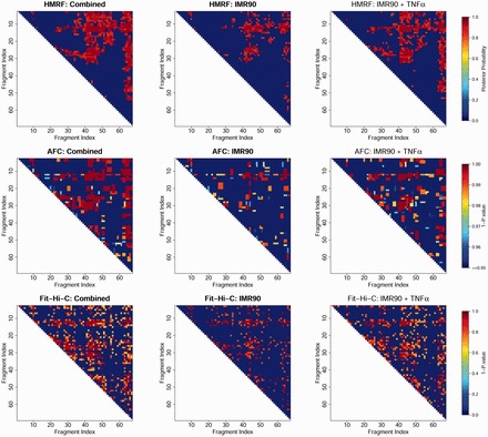
Peaks called in the domain Chr.17:29.52 Mb-29.72 Mb. For each dataset (combined, before and after TNF-α treatment), the same number of peaks as using AFC method was shown (based on posterior probabilities for HMRF and P-values for Fit-Hi-C) for comparison

Table 1.

Genome-wide real data evaluation based on false-positive rate (FPR), false discovery rate (FDR) and recover rate (RR)

Dataset		Method		FPR (%)		FDR (%)		RR (%)
IMR90		HMRF-Bayesian		0.52		15.60		42.30
IMR90		AFC		0.60		18.40		41.10
IMR90		Fit-Hi-C		0.64		19.20		41.20
IMR90 + TNF-α		HMRF-Bayesian		0.83		18.50		55.40
IMR90 + TNF-α		AFC		0.98		22.40		52.90
IMR90 + TNF-α		Fit-Hi-C		1.00		22.50		53.30
Dataset		Method		FPR		FDR		RR
Split1		HMRF		0.84		19.10		55.90
Split1		AFC		0.97		22.60		54.00
Split1		Fit-Hi-C		1.03		23.50		53.70
Split2		HMRF		0.47		15.20		41.30
Split2		AFC		0.56		18.60		39.90
Split2		Fit-Hi-C		0.58		18.80		40.30

Assuming calling result for the combined dataset is the true peak pattern, we summarized the following measures for 1432 domains, i.e. genome-wide. We reported the genome-wide average of false-positive rate (FPR), false discovery rate (FDR) and recovery rate (RR) by the HMRF-Bayesian method, AFC method and Fit-Hi-C for both IMR90 before TNF-α treatment and IMR90 after TNF-α treatment. We found that the HMRF-Bayesian method has better performance than AFC method and Fit-Hi-C

Table 2.

Genome-wide real data evaluation based on the consistency measure (Jaccard Index)

Method	IMR90 vs. IMR90 + TNF-α* (%)	Split1 vs Split2* (%)
HMRF	22.1 ± 0.33	22.7 ± 0.32
AFC	18.4 ± 0.32	18.5 ± 0.31
Fit-Hi-C	13.7 ± 0.29	13.6 ± 0.28

*Mean ± SE

We next proceeded to quantitatively and systematically evaluate the performance based on genome-wide calling for all domains. For a fair comparison, we selected thresholds based on posterior peak probabilities for our method and P-values for Fit-Hi-C to match the number of peaks called by AFC for each dataset. We also performed other comparisons where we matched the number of peaks called by either our method or Fit-Hi-C, or where we let each method call peaks according to its own criterion and found similar patterns (detailed in Supplementary Material Section 5). Treating peaks called in the combined dataset as truth, we gauged performance in single-condition datasets using the following three statistics: false-positive rate (FPR), false discovery rate (FDR) and recovery rate (RR). Denote the number of false positives, true positives, false negatives and true negatives as FP, TP, FN and TN, where the truth is defined according to AFC results from the combined dataset and the four numbers sum up to the total number of intra-domain fragment pairs. We have FPR = FP/(FP + TN), FDR = FP/(FP + TP) and RR = TP/(TP + TN). As shown in Table 1 upper panel, methods accounting for potential dependency of underlying peak statuses (AFC and our HMRF Bayesian caller) resulted in better performance than Fit-Hi-C which models fragment pairs independently. Furthermore, our method outperformed the others for all three measures. For example, for IMR90 before TNF-α treatment, we obtained FPR = 0.52%, FDR = 15.6% and RR = 42.3% for our HMRF Bayesian caller, compared with FPR = 0.60%, FDR = 18.4% and RR = 41.1% for AFC and FPR = 0.64%, FDR = 19.2% and RR = 41.2% for Fit-Hi-C. By borrowing information from neighboring fragment pairs in a probabilistic framework, our method lead to more robust inference with simultaneously lower false positive, false discovery rates and higher recovery rate.

In addition, for each caller, we calculated the Jaccard Index (Hamers et al., 1989) between the peak sets from the two conditions, defined as the ratio of number of peaks identified under both conditions over the number of peaks identified by either. Average Jaccard Index across all domains genome-wide is shown in Table 2 for each method. Again, methods accounting for the dependency of underlying peak status show higher concordance across conditions. Average Jaccard Index improved by 33.6% and 61.3% respectively, from 13.7% (Fit-Hi-C) to 18.4% (AFC) and 22.1% (HMRF).

To avoid potential systematic differences between treated and untreated conditions in terms of peak status (although not supported by results in Jin et al. (2013)), we also analyzed two randomly split datasets as described by Jin et al. (2013). Results shown in Table 1 (lower panel) and Table 2 (rightmost column) similarly show better reproducibility and robustness of our methods over existing ones.

Given one important utility of called peaks is to illuminate biologically meaningful interactions, we directly evaluated the power to identify one important category of biological interactions: between enhancers and transcription start sites (TSS). We used the enhancer-promoter connection map based on multi-tissue correlations between distal and promoter chromatin accessibility (Thurman et al., 2012), augmented with results from multi-tissue correlations between chromatin accessibility and gene expression (Sheffield et al., 2013), retrieved from http://dnase.med.unc.edu/supplement/allGeneCorrelations100000.p2.txt.gz. We left Fit-Hi-C out in the comparison as it showed incomparable reproducibility with the other callers. Supplementary Figure S4 demonstrates the increased power of HMRF over AFC with up to 11.3% more enhancer-TSS interactions identified by HMRF, given the same number of peak regions called by two methods. In addition, Supplementary Figure S5 shows one particular example where the potential target gene CTSB (Maurano et al., 2012) of a GWAS variant rs1600249 (Freudenberg et al., 2011) was missed by AFC but captured by our method.

In addition, we performed transcription factor binding sites (TFBS) and active TSS (reported by Jin et al., 2013) enrichment analysis to elucidate the biological relevance of identified interactions. Specifically, we evaluated two aspects. First, we tested if fragment pairs detected as interacting loci are enriched with TFBS. Second, we compared the number of interacting loci for TFBS versus non-TFBS. We used ENCODE IMR90 TFBS information retrieved from http://hgdownload.cse.ucsc.edu/goldenpath/hg19/encodeDCC/wgEncodeRegTfbsClustered where TFBS were called from ChIP-seq data using the computational pipeline developed by the ENCODE project (Gerstein et al., 2012; Wang et al., 2013). We found that regardless of the detection threshold (ranging from 1 in 100 000 fragment pairs called as peaks to 1 in 100), the pairs of interacting fragments called are significantly enriched with TFBS and active TSS (${\text{χ}}^2$P-value < ${10}^{-238})$ with ∼42% identified peak pairs overlapping with TFBS while ∼28% identified non-peak pairs overlapping with TFBS (Fig. 2 ). In addition, we found that fragments overlapping with TFBS or active TSS are involved in a slightly (but statistically significant) larger number of interactions than those not overlapping with TFBS or active TSS (Supplementary Fig. S6).

Fig. 2.

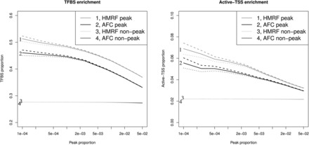
TFBS and active-TSS enrichment. Solid lines are estimated average levels. The 95% confidence interval of estimated average levels are represented by dashed lines and solid lines. Left panel: TFBS enrichment analysis. Right panel: active-TSS enrichment analysis

Finally, we applied our methods to two other datasets: the mouse embryonic stem cell (mESC) and human embryonic stem cell (H1-hESC) dataset (Dixon et al., 2012). For both datasets, we downloaded observed Hi-C count data from the Fit-Hi-C website and estimated the expected counts using Fit-Hi-C. For mESC, genome-wide ChIA-PET data are available (Zhang et al., 2013) and for H1-hESC, 5C data were generated in 44 regions by the ENCODE pilot project (Sanyal et al., 2012). We gauged performance of our methods and of Fit-Hi-C by comparison with results from data generated from independent technologies. Comparison results suggest our method was able to detect more interactions captured from 5C (Supplementary Fig. S7a) or ChIA-PET (Supplementary Fig. S7b) data with the same number of peak regions called, according to HMRF posterior peak probabilities or Fit-Hi-C P-values.

4 Discussion

Peak calling from data generated by 3C-derived methods is a fundamental task for the identification of chromatin interactions in 3D space. However, model-based methods for this important task are still lacking. Existing methods focus on the calibration of expected count frequency distribution under random collision, accounting for multiple biases behind 3C analysis including but not limited to density of restriction enzyme sites, mappability and GC content. We have found existing methods rather mature for the purpose of calibrating expected counts (with results robust to different methods used). Establishing the expected count distribution is nevertheless a prerequisite, not peak calling itself. None of the existing methods consider the dependency underlying the peak status with statistical rigor.

In this work, we propose a HMRF based Bayesian method that explicitly models the dependency of the underlying peak pattern. The true peak pattern is unknown and can take different forms in the presence of dependency. We simplify the problem by assuming an Ising distribution prior and learn the level of dependency from data in a Bayesian framework. Our extensive simulations indicate superior performance in terms of both the estimation of the extent of dependency and the statistical power to distinguish peaks from background, across a range of underlying dependency patterns.

There are several aspects where the model can be further elaborated. First, our model has one $\theta$, one $\psi$ and one $\varphi$, thus assuming that peaks are of similar strength and clustering patterns, and that reads have similar levels of over-dispersion. While the first two are simplifying assumptions bypassing issues including model selection difficulty and parameter non-identifiability, the last has been shown to be reasonable (Jin et al., 2013). Sensitivity analysis with the IMR90 combined dataset suggests these assumptions are reasonable: splitting each domain into two equal sub-domains resulted in highly consistent peak calls (Spearman correlation > 0.9, detailed in Supplementary Material Section 4). Second, we use a one-parameter Ising prior, with the parameter controlling both the peak proportion and level of dependency. A two-parameter Ising prior would allow more flexibility, particularly when the underlying dependency is weak. Third, our method could allow incorporation of prior knowledge, when available, into the model. For instance, a hyper prior could be imposed on the inverse temperature parameter based on estimated distribution from similar existing datasets. Finally, the computational complexity of our Bayesian modeling is quadratic in terms of the number of fragments under consideration. Our JAVA implementation takes ∼13 minutes for a typical domain with 200 fragments and with parallel computing, genome-wide analysis can be easily accomplished within a few hours. In contrast, Fit-Hi-C and our R implementation of AFC take ∼4 seconds and ∼12 minutes, respectively. Therefore, for future work, computationally more efficient algorithms warrant consideration. We attempted to apply the iterative conditional mode algorithm (Li et al., 2010), but observed unsatisfactory performance with weak peak signals (data not shown).

Despite these possible further model improvements, our method has demonstrated favorable performance over existing methods by borrowing information from neighboring fragment pairs via statistically modeling the potential dependency among the underlying peaks using a Bayesian framework. Our extensive simulation studies (Supplementary Material Section 2) show the advantage of our method across a range of dependency patterns and its ability to learn the level of dependency (as modeled by the inverse temperature parameter) from data. Both are valuable since we have limited, if any, prior knowledge regarding the extent of dependency in real data. Re-analysis of several published Hi-C datasets including the IMR90, H1-hESC and mESC data confirmed the value of dependency modeling as taking dependency into consideration resulted in better concordance (>40% improvement as measured by Jaccard Index of peak sets across two IMR90 datasets) and lower false positive, false discovery rates and higher recovery rate. Our method is the first to model dependency in a statistically rigorous manner and to borrow information from neighboring fragment pairs through a probabilistic model, was able to call up to 11.3% more enhancer-TSS interactions than the ad hoc method given the same number of peak regions called. We acknowledge that there is currently no genome-wide gold standard for real data (for example, from large scale genome-wide imaging-based experiments). We therefore made special efforts to benchmark the methods across multiple datasets and for each dataset, against the most reasonable silver standard. For example, for the IMR90 cell lines, we compared against results from the combined dataset with the highest sequencing depth, for H1 hESC and mESC, we used results from independent technologies (5C and ChIA-PET, respectively).

With the continuing drop in sequencing costs and the intensive interest in chromatin structure as a way to understand GWAS results, we anticipate in the near future more high-resolution (fragment-level) Hi-C data where our method have demonstrated key advantage given the non-negligible dependency structure.

Funding

This research was supported by research grants R01HG006292, R01HG006703, R01DA030976, R01HG005119 and U54DK107977.

Conflict of Interest: none declared.

References

- Ay F., et al. (2014) Statistical confidence estimation for Hi-C data reveals regulatory chromatin contacts. Genome Res., 24, 999–1011. [DOI] [PMC free article] [PubMed] [Google Scholar]
- Bau D., et al. (2011) The three-dimensional folding of the alpha-globin gene domain reveals formation of chromatin globules. Nat. Struc. Mol. Biol., 18, 107–114. [DOI] [PMC free article] [PubMed] [Google Scholar]
- Besag J., et al. (1995) Bayesian computation and stochastic-systems. Stat. Sci., 10, 3–41. [Google Scholar]
- Bernstein B.E., et al. (2012) An integrated encyclopedia of DNA elements in the human genome. Nature, 489, 57–74. [DOI] [PMC free article] [PubMed] [Google Scholar]
- Choi H., et al. (2010) A double-layered mixture model for the joint analysis of DNA copy number and gene expression data. J. Comput. Biol., 17, 121–137. [DOI] [PMC free article] [PubMed] [Google Scholar]
- Dekker J., et al. (2013) Exploring the three-dimensional organization of genomes: interpreting chromatin interaction data. Nat. Rev. Genet., 14, 390–403. [DOI] [PMC free article] [PubMed] [Google Scholar]
- Dekker J., et al. (2002) Capturing chromosome conformation. Science, 295, 1306–1311. [DOI] [PubMed] [Google Scholar]
- Dixon J.R., et al. (2012) Topological domains in mammalian genomes identified by analysis of chromatin interactions. Nature, 485, 376–380. [DOI] [PMC free article] [PubMed] [Google Scholar]
- Duan Z., et al. (2010) A three-dimensional model of the yeast genome. Nature, 465, 363–367. [DOI] [PMC free article] [PubMed] [Google Scholar]
- François O., et al. (2006) Bayesian clustering using hidden Markov random fields in spatial population genetics. Genetics, 174, 805–816. [DOI] [PMC free article] [PubMed] [Google Scholar]
- Freudenberg J., et al. (2011) Genome-wide association study of rheumatoid arthritis in Koreans. Arthritis. Rheum. US, 63, 884–893. [DOI] [PubMed] [Google Scholar]
- Gelman A. (2004) Bayesian data analysis. Boca Raton, FL: Chapman & Hall/CRC. [Google Scholar]
- Gerstein M.B., et al. (2012) Architecture of the human regulatory network derived from ENCODE data. Nature, 489, 91–100. [DOI] [PMC free article] [PubMed] [Google Scholar]
- Hamers L., et al. (1989) Similarity measures in scientometric research – the Jaccard Index versus Salton Cosine Formula. Inform. Process. Manag., 25, 315–318. [Google Scholar]
- Hindorff L.A., et al. (2009) Potential etiologic and functional implications of genome-wide association loci for human diseases and traits. Proc. Natl. Acad. Sci. USA, 106, 9362–9367. [DOI] [PMC free article] [PubMed] [Google Scholar]
- Hou C.H., et al. (2012) Gene density, transcription, and insulators contribute to the partition of the drosophila genome into physical domains. Mol. Cell, 48, 471–484. [DOI] [PMC free article] [PubMed] [Google Scholar]
- Hu M., et al. (2013) Bayesian inference of spatial organizations of chromosomes. Plos Comput. Biol., 9, e1002893. [DOI] [PMC free article] [PubMed] [Google Scholar]
- Imakaev M., et al. (2012) Iterative correction of Hi-C data reveals hallmarks of chromosome organization. Nat. Methods, 9, 999. [DOI] [PMC free article] [PubMed] [Google Scholar]
- Jhunjhunwala S., et al. (2008) The 3D structure of the immunoglobulin heavy-chain locus: implications for long-range genomic interactions. Cell, 133, 265–279. [DOI] [PMC free article] [PubMed] [Google Scholar]
- Jin F., et al. (2013) A high-resolution map of the three-dimensional chromatin interactome in human cells. Nature, 503, 290–294. [DOI] [PMC free article] [PubMed] [Google Scholar]
- Kindermann R., et al. (1980) Markov random fields and their applications. Providence, RI: American Mathematical Society. [Google Scholar]
- Kumar V., et al. (2012) From genome-wide association studies to disease mechanisms: celiac disease as a model for autoimmune diseases. Semin. Immunopathol., 34, 567–580. [DOI] [PMC free article] [PubMed] [Google Scholar]
- Li G.L., et al. (2012) Extensive promoter-centered chromatin interactions provide a topological basis for transcription regulation. Cell, 148, 84–98. [DOI] [PMC free article] [PubMed] [Google Scholar]
- Li H.Z., et al. (2010) A hidden Markov random field model for genome-wide association studies. Biostatistics, 11, 139–150. [DOI] [PMC free article] [PubMed] [Google Scholar]
- Lieberman-Aiden E., et al. (2009) Comprehensive mapping of long-range interactions reveals folding principles of the human genome. Science, 326, 289–293. [DOI] [PMC free article] [PubMed] [Google Scholar]
- Marti-Renom M.A., Mirny L.A. (2011) Bridging the resolution gap in structural modeling of 3d genome organization. Plos Comput. Biol., 7, e1002125. [DOI] [PMC free article] [PubMed] [Google Scholar]
- Maurano M.T., et al. (2012) Systematic localization of common disease-associated variation in regulatory DNA. Science, 337, 1190–1195. [DOI] [PMC free article] [PubMed] [Google Scholar]
- Mo Q.X. (2012) A fully Bayesian hidden Ising model for ChIP-seq data analysis. Biostatistics, 13, 113–128. [DOI] [PubMed] [Google Scholar]
- Niu L., et al. (2014) Statistical models for detecting differential chromatin interactions mediated by a protein. Plos One, 9, e97560. [DOI] [PMC free article] [PubMed] [Google Scholar]
- Nora E.P., et al. (2012) Spatial partitioning of the regulatory landscape of the X-inactivation centre. Nature, 485, 381–385. [DOI] [PMC free article] [PubMed] [Google Scholar]
- Pennisi E. (2011) The biology of genomes. Disease risk links to gene regulation. Science, 332, 1031. [DOI] [PubMed] [Google Scholar]
- Qin Z.H.S., et al. (2010) HPeak: an HMM-based algorithm for defining read-enriched regions in ChIP-Seq data. BMC Bioinformatics, 11, 369. [DOI] [PMC free article] [PubMed] [Google Scholar]
- Russel D., et al. (2012) Putting the pieces together: integrative modeling platform software for structure determination of macromolecular assemblies. Plos Biol., 10, e1001244. [DOI] [PMC free article] [PubMed] [Google Scholar]
- Sajan S.A., Hawkins R.D. (2012) Methods for identifying higher-order chromatin structure. Annu. Rev. Genomics Hum. Genet., 13, 59–82. [DOI] [PubMed] [Google Scholar]
- Sanyal A., et al. (2012) The long-range interaction landscape of gene promoters. Nature, 489, 109–113. [DOI] [PMC free article] [PubMed] [Google Scholar]
- Sexton T., et al. (2012) Three-dimensional folding and functional organization principles of the drosophila genome. Cell, 148, 458–472. [DOI] [PubMed] [Google Scholar]
- Sheffield N.C., et al. (2013) Patterns of regulatory activity across diverse human cell types predict tissue identity, transcription factor binding, and long-range interactions. Genome Res., 23, 777–788. [DOI] [PMC free article] [PubMed] [Google Scholar]
- Smallwood A., Ren B. (2013) Genome organization and long-range regulation of gene expression by enhancers. Curr. Opin. Cell Biol., 25, 387–394. [DOI] [PMC free article] [PubMed] [Google Scholar]
- Smemo S., et al. (2014) Obesity-associated variants within FTO form long-range functional connections with IRX3. Nature, 507, 371. [DOI] [PMC free article] [PubMed] [Google Scholar]
- Stingo F.C., Vannucci M. (2011) Variable selection for discriminant analysis with Markov random field priors for the analysis of microarray data. Bioinformatics, 27, 495–501. [DOI] [PMC free article] [PubMed] [Google Scholar]
- Thurman R.E., et al. (2012) The accessible chromatin landscape of the human genome. Nature, 489, 75–82. [DOI] [PMC free article] [PubMed] [Google Scholar]
- Trieu T., Cheng J. (2014) Large-scale reconstruction of 3D structures of human chromosomes from chromosomal contact data. Nucleic Acids Res, 42, e52. [DOI] [PMC free article] [PubMed] [Google Scholar]
- Wang J., et al. (2013) Factorbook.org: a Wiki-based database for transcription factor-binding data generated by the ENCODE consortium. Nucleic Acids Res., 41, D171–D176. [DOI] [PMC free article] [PubMed] [Google Scholar]
- Ward L.D., Kellis M. (2012) Interpreting noncoding genetic variation in complex traits and human disease. Nat. Biotechnol., 30, 1095–1106. [DOI] [PMC free article] [PubMed] [Google Scholar]
- Wei P., Pan W. (2010) Network-based genomic discovery: application and comparison of Markov random-field models. J. R. Stat. Soc. C Appl., 59, 105–125. [DOI] [PMC free article] [PubMed] [Google Scholar]
- Zhang Y., et al. (2013) Chromatin connectivity maps reveal dynamic promoter-enhancer long-range associations. Nature, 504, 306–310. [DOI] [PMC free article] [PubMed] [Google Scholar]
Associated Data
This section collects any data citations, data availability statements, or supplementary materials included in this article.