A quantitative model for oxygen uptake and release in a family of hemeproteins

Abstract

Motivation: Hemeproteins have many diverse functions that largely depend on the rate at which they uptake or release small ligands, like oxygen. These proteins have been extensively studied using either simulations or experiments, albeit only qualitatively and one or two proteins at a time.

Results: We present a physical–chemical model, which uses data obtained exclusively from computer simulations, to describe the uptake and release of oxygen in a family of hemeproteins, called truncated hemoglobins (trHbs). Through a rigorous statistical analysis we demonstrate that our model successfully recaptures all the reported experimental oxygen association and dissociation kinetic rate constants, thus allowing us to establish the key factors that determine the rates at which these hemeproteins uptake and release oxygen. We found that internal tunnels as well as the distal site water molecules control ligand uptake, whereas oxygen stabilization by distal site residues controls ligand release. Because these rates largely determine the functions of these hemeproteins, these approaches will also be important tools in characterizing the trHbs members with unknown functions.

Contact: lboechi@ic.fcen.uba.ar

Supplementary information: Supplementary data are available at Bioinformatics online.

1 Introduction

The combination of computer simulations and biochemical experiments has become a reliable strategy to describe the underlying molecular details of observed differences in the activity of proteins. With an increasing amount of data on individual proteins, the construction of mathematical models that permit a more generalized understanding of these molecular details has become a challenge of interest to many groups around the world (Oliveira et al., 2014; Potapov et al., 2015; Pucci and Rooman, 2014; Silk et al., 2014). The truncated hemoglobins (trHbs) are a family of hemeproteins that share a conserved three-dimensional structure as well as the structural positions of their active site residues (Wittenberg et al., 2002). Their diverse functions are related to their ability to uptake and release ligands with a wide range of entry and exit rates. Because the ligands bind to the heme group, which is buried in the protein, the ligand entry and exit rates depend to a great extent on the ligands ability to migrate to and from the active site via three potential tunnels in the protein matrix (Elber, 2010; Milani et al., 2001; Perutz and Mathews, 1966), as shown in Figure 1A. Each protein may present one or two open tunnels, lined by particular residues defining its topology. Protein cavities have been identified several decades ago through experiments in a Xe atmosphere, where protein sites with retained Xe atoms were identified. In the case of myoglobin, for example, several studies had demonstrated the importance of internal cavities as ligand hosts as well as part of migratory tunnels (Brunori, 2000; Brunori et al., 2000; Scott et al., 2001). Crystallographic studies of trHbs from Mycobacterium tuberculosis, Chlamydomonas eugametos and Paramecium caudatum also highlight the importance of these cavities in the trHb protein family (Milani et al., 2004; Mishra and Meuwly, 2009). Several studies have shown that in addition to the presence and nature of these migratory tunnels, certain active site residues can also modulate ligand entry and exit, in particular, delaying ligand entry by stabilizing water molecules that block accessibility to the heme (Fig. 1B), (Bustamante et al., 2014; Goldbeck et al., 2006; Olson and Phillips, 1997; Ouellet et al., 2008; Scott et al., 2001) or by delaying ligand exit by stabilizing the ligand itself (Fig. 1C) (Capece et al., 2013; Lu et al., 2007; Ouellet et al., 2003, 2007a). Experimentally, it is possible to characterize ligand entry and exit by measuring the ligand association (k_on) and dissociation (k_off) kinetic rate constants, respectively. Specifically, k_on determines the rate at which the ligand reaches the protein heme iron from outside the protein, and k_off determines the rate at which the ligand is released once it is bound to the iron. Both k_on and k_off have been reported for a number of members of the trHb family (Bonamore et al., 2005; Bustamante et al., 2014; Couture et al., 1999, 2000; Das et al., 2000; Giordano et al., 2011; Goldbeck et al., 2006; Lu et al., 2007; Olson and Phillips, 1997; Ouellet et al., 2003, 2006, 2007b, 2008; Watts et al., 2001). Though the trHb family (with ∼1100 members) has only recently been identified, a subset of ∼10 members and several mutants have been characterized extensively by both biochemical experiments and computer simulations (Chodera et al., 2011; Dinner et al., 2000; Elber, 2010; Perilla et al., 2015; Sotomayor and Schulten, 2007). In this study, we utilize data from single-molecule computer simulations of these hemeproteins to build a theoretical model that is in statistical agreement with all the oxygen k_on and k_off values reported in the literature. Namely, all variables involved in the model are relevant (corresponding coefficients are statistically significant), model assumptions for quantifications are not violated and the model achieves a high predictive ability. Considering the accuracy of this model we are able to confirm the main factors that control both ligand entry and exit for all the members studied and, further, propose two quantitative approaches for predicting the oxygen association and dissociation rate constants for the rest of the family members. Because these rates largely determine the functions of these hemeproteins, these approaches will be important tools in characterizing trHb members with unknown functions. Based on our model, we propose strategies for predicting both the oxygen association and dissociation rate constants for the rest of the family members, which allows the development of whole family evolutionary and functional studies, as shown in Bustamante et al. (2016).

Fig. 1.

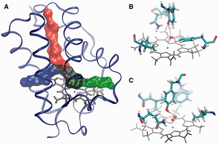
Representation of a typical trHb, their possible tunnels and active site. (A) Schematic representation of the potential three tunnels (red, blue and green) that connect the solvent with the active site in trHbs. Cartoon representations of the active site in the trHbN of M. tuberculosis, the heme group (grey), with key amino acids, water (B), and oxygen (C) stabilized by HBs (dotted lines) shown as ball-and-sticks (Color version of this figure is available at Bioinformatics online.)

2 Methods

2.1 Set up of the systems and classical simulation parameters

The protein structures for all herein studied cases correspond to the following PDBids: 1IDR (Milani et al., 2001) (Mt-trHbN, from M.tuberculosis), 1NGK (Milani et al., 2003) (Mt-trHbO), 2BMM (Bonamore et al., 2005) (Tf-trHbO, from Thermobifida fusca), 4UUR (Giordano et al., 2015) (Ph-trHbO, from Pseudoalteromonas haloplanktis), 2XYK (Pesce et al., 2011) (At-trHbO, from Agrobacterium tumefaciens), 1UX8 (Giangiacomo et al., 2005) (Bs-trHbO, from Bacillus subtilis), 1DLY (Pesce et al., 2000) (Ce-trHbN, from C.eugametos), 1DLW (Pesce et al., 2000) (Pc-trHbN, from P.caudatum), 2BKM (Ilari et al., 2007) (Gs-trHbO from Geobacillus stearothermophilus), 1RTX (Hoy et al., 2004) (Syn-trHbN from Synechocystis), 2IG3 (Nardini et al., 2006) (Cj-trHbP from Campylobacter jejuni) and 1VXG (Yang and Phillips Jr., 1996) (sperm whale myoglobin). In all cases, the systems were built and simulated according to the protocol of Giordano et al. (2015). An unconstrained 50 ns molecular dynamics (MD) simulation at constant temperature (300 K) was performed for each simulated system. In silico mutant proteins, i.e. single and double mutants of some wild type (wt) forms, were built starting from the same crystal structure as described above and mutated then using the tLEaP module of the AMBER12 package (Pearlman et al., 1995). These mutant structures were equilibrated and simulated using the same protocol as that used for the wt form. All structures were found to be stable during the timescale of simulations, as evidenced by the Root Mean Square Deviation analyses (data not shown).

2.2 Oxygen migration free energy profiles

Free energy profiles for the O₂ migration process along the protein tunnel/cavity system were computed using the Implicit Ligand Sampling (ILS) approach (Cohen et al., 2006, 2008), which has been widely used to study these process and was shown previously by our group to yield accurate results (Boron et al., 2015; Bustamante et al., 2014; Forti et al., 2011; Marcelli et al., 2012). In Supplementary Figure S1, a comparison of O₂ migration over the same trHbs, sampled with both classical MD with a free explicit oxygen molecule as well as with an implicit O₂ molecule under the ILS method is shown. We found that smaller barriers calculated by ILS method correspond to higher entry and exit rates by using classical MD with explicit oxygen. In addition, our calculations agree with previous calculations of trHbs such as Mt-trHbN and Mt-trHbO already reported using different methods (Bidon-Chanal et al., 2006; Boechi et al., 2008; Cazade and Meuwly, 2012; Guallar et al., 2009; Mishra and Meuwly, 2009). ILS calculations were performed in a rectangular grid (0.5 Å resolution) that includes the whole simulation box (i.e. protein and the solvent), the used probe was an O₂ molecule. Calculations were performed on 5000 frames taken from the 50 ns of the production simulations. The values for grid size, resolution and frame numbers were thoroughly tested in our previous work (Forti et al., 2011). Analysis of the ILS data was performed using an adhoc TCL program available under request, determining in each case the magnitude of the corresponding wells and barriers scaled, so that the free energy of the ligand in the bulk solvent is set to 0. In order to present evidence of the ILS convergence, a plot of the maximum free energy values along 250 ns for trHbs N and O from M.tuberculosis as representative examples is shown (Supplementary Fig. S2).

2.3 Oxygen binding energy (Δ$E_{{\text{O}}_2}$)

QM-MM calculations were performed by geometry optimization of a selected representative snapshot extracted from the MD simulations. To select this representative snapshot we analyzed the hydrogen bond (HB) network that stabilizes the O₂ molecule. In cases where this network presented more than one stable conformation, both conformations were considered as representative snapshots and the overall Δ$E_{{\text{O}}_2}$ value was calculated as an average of the two computed Δ$E_{{\text{O}}_2}$ values. The quantum part consisted of the heme moiety without the carboxylic side chains, plus the proximal histidine and the oxygen molecule. We have set the spin states of the iron according to the experimental ones, singlet and quintuplet states for the oxy and deoxy species, respectively. Even if O₂ binding to heme is a complex phenomenon and thus, an adequate quantitative description requires high level abinitio multi-configurational schemes (Kepp, 2013), DFT calculations yield reasonable comparative results and have proven to achieve reliable results in a variety of heme proteins in previous works from our group (Capece et al., 2013).

O₂ binding energies (Δ$E_{{\text{O}}_2}$, kcal/mol) were calculated as:

$$\Delta E_{{\text{Prot-O}}_2}-(E_{{\text{O}}_2}+E_{\text{Prot}}),$$ (1)

where $E_{{\text{Prot-O}}_2}$ is the energy of the oxygenated protein, E_Prot is the energy of the deoxygenated protein and $E_{{\text{O}}_2}$ is the energy of the isolated oxygen molecule. The oxygenated proteins were simulated in the singlet spin state, the deoxygenated proteins in the quintet spin state and the free oxygen in the triplet state, which are the known ground states for each case. All simulations were performed at the unrestricted spin approximation. This method strategy has been widely and successfully used in our group to study oxygen (as well as other ligands) affinity in previous works (Capece et al., 2013). It is well known that computed oxygen dissociation energies from the heme are significantly overestimated due to the fact that a low (singlet) to high spin (quintet) transition is involved and DFT overestimates the energy of the spin gap, favoring low spin configurations (Scherlis et al., 2007). On the other hand, Δ$E_{{\text{O}}_2}$ values are computed for the optimized, i.e. best possible conformation at 0 K, and kinetic values are computed at room temperature. Due to intrinsic errors of the DFT-based QM/MM methods, the computed energies are strongly dependent on the exchange-correlation functional and basis set. All these issues can be partially corrected standardizing the oxygen binding energy. To do so, we define $\Delta \Delta E_{{\text{O}}_2}$, that corresponds to the Δ$E_{{\text{O}}_2}$ (oxygen binding energy computed as described above in Equation 1) and the difference between ΔE_heme, the calculated oxygen binding energy of an isolated imidazol bound heme in vacuum (which is 22 kcal/mol at this level of theory) and free heme k_off value (10⁴ s ⁻¹) (Marti et al., 2006; Scott et al., 2001).

3 Results

3.1 Modeling the ligand association rate constant (k_on)

The Eyring equation is widely used to model bimolecular reactions in the context of transition state theory:

$$k=\frac{k_{\text{B}}T}{h}·e^{-\frac{\Delta G^{‡}}{RT}},$$ (2)

where ΔG^‡ is the Gibbs energy of activation, T is the temperature, $k_{\text{B}}$, h and R are the Boltzmann, Planck and the universal gas constants, respectively.

In our case, we constructed an Eyring model that includes the free energy barrier to ligand entry through migratory tunnels, as well as the free energy penalty for removing a water molecule from the active site.

In our model, each tunnel or gate was considered independently for each trHb, taking into account that in every case one tunnel was significantly more accessible than the others. In this sense, the highest barrier of the most accessible tunnel was considered as the free energy barrier for oxygen entry, denoted Δ${\text{G}}_{\text{in}}^{‡}$. This allows us to use a pure simple statistical analysis, starting from a parsimonious model. Because water molecules in the active site are stabilized through HB interactions, the free energy of removing a water molecule was approximated as the product between the number of HB interactions ($n_{\text{HB}}$) between the water molecule and the surrounding active site residues and the free energy of an HB interaction (ΔG_HB). We performed 50 ns of classical MD simulations with explicit solvent molecules (that is ∼5000 water molecules around the protein), allowing water molecules to explore and thus occupy key active site positions. The n_HB value was calculated as the average number of hydrogen bound during those simulations. The individual contributions of $\Delta G_{\text{in}}^{‡}$ and $n_{\text{HB}}$ were then combined in the following physical–chemical model for the theoretical value of k_on:

$$k_{\text{on}}=\frac{k_{\text{B}}T}{h}·e^{-\frac{\Delta G_{\text{in}}^{‡}}{RT}}·e^{-\frac{\Delta G_{\text{HB}}·n_{\text{HB}}}{RT}},$$ (3)

where T  = 300 K. The value of ΔG_HB is a constant in the model, however, because different values for ΔG_HB have been reported in the literature (between 2 and 5 kcal/mol), depending on the immediate environment, it is not possible for us to provide at this point value of ΔG_HB in our model (Markovitch and Agmon, 2007).

We will consider the logarithm form of Equation (3), such that it becomes a linear model. All logarithms involved in the study are in base 10. If we further assume that each experimental value for each protein differs from the theoretical k_on by an additive random error (ϵi), we arrive at the following statistical model:

$$\log {(k_{\text{on}})}_i=\log \left(\frac{k_{\text{B}}T}{h}\right)+\frac{(-1)}{RT}·\log (e)·\Delta G_{{\text{in}}_i}^{‡}+\frac{(-\Delta G_{\text{HB}})}{RT}·\log (e)·n_{{\text{HB}}_i}+{ϵ}_i,$$ (4)

where the index i corresponds to the i^th protein. We note that the random error (${\mathrm{ϵ}}_{\text{i}}$) accounts for measurement errors, biological variability and possible misconceptions or incompleteness in the model. The randomness of the error term ${\mathrm{ϵ}}_{\text{i}}$ in Equation (4) turns this equation into a first statistical model, in the sense that it combines our knowledge of the chemistry of the problem with the uncertainty enclosed by the error.

There are two aspects involved in the construction of model (4). On the one hand, the model suggests that $\Delta G_{\text{in}}^{‡}$ and $n_{\text{HB}}$ are the variables that allow to linearly describe the behavior (in logarithm form) of k_on. On the other hand, it establishes in which ways these variables should be combined, by determining the value of the coefficient that accompanies $\Delta G_{\text{in}}^{‡}$ as well as the intercept, $\log (k_{\text{B}}T/h)$.

To statistically validate each of these two aspects, we postulate that $\log (k_{\text{on}})$ can be expressed as a linear combination of both predictors ($\Delta {\text{G}}_{\text{in}}^{‡}$ and $n_{\text{HB}}$), up to a random error term. Now, in contrast to Equation (4), no restrictions on the coefficients are imposed. This gives rise to the following statistical model:

$$\log {(k_{\text{on}})}_i={\beta }_0+\frac{{\beta }_1}{RT}·\log (e)·\Delta {\text{G}}_{{\text{in}}_i}^{‡}+\frac{{\beta }_2}{RT}·\log (e)·n_{{\text{HB}}_i}+{ϵ}_i.$$ (5)

In addition, the errors are assumed to be Gaussian distributed with mean 0 and constant standard deviation (linear model assumptions). Model (5) does not specify values for the coefficients β_j, j  =  0, 1, 2. However, if we let ${\beta }_0=\log (k_{\text{B}}T/h),{\beta }_1=-1$ and ${\beta }_2=-\Delta$G_HB in model (5), we would recover model (4).

Note that β₁ is a scaling factor that determines if the calculated value for $\Delta {\text{G}}_{\text{in}}^{‡}$ is overestimated or underestimated, whereas β₂ corresponds to the free energy of an HB interaction.

We adjust model (5) to obtain the best linear model for the reported k_on values for trHbs and Mb (n = 26). Table 1 summarizes the results of the fit. There were no constraints imposed on the coefficients β₀, β₁ and β₂, such that they were free to take any value. Finding the best fit to model (5) by least square regression we can evaluate both the accuracy of the linear description of $\log (k_{\text{on}})$ with the considered variables $\Delta {\text{G}}_{\text{in}}^{‡}$ and $n_{\text{HB}}$, as well as the proposed values for the coefficients in model (4).

Table 1.

Estimated values for the coefficients with their respective 95% confidence intervals and P-values for model (5)

Equation	Best fit coefficient	Proposed coefficients	Estimated value and 95% CI	P-values
(5) (R2 = 0.78)	β 0	log(kBT/h) = 12.769	11.81 ± 1.15	<2 × 10−16
	β 1	ΔG‡in coeff. = −1	−1.25 ± 0.40	1.65 × 10−6
	β 2	−ΔGHB ∈ [−5, −2]	−1.99 ± 0.50	3.14 × 10−8

The linear model turned out to be accurate in describing the relation between the involved variables. The R² was found to be 0.78, meaning that 78% of the variability of $\log (k_{\text{on}})$ can be explained at a linear level in terms of both explicative variables. The estimated standard deviation of the error ϵ_i for model (5) was 0.56, which is really small compared with the values observed for the response variable ($\log (k_{\text{on}})$), which range from ∼5 to 10.

All coefficients, β₀, β₁ and β₂, were found to be statistically significant (the corresponding P-values are <0.05), which means that there is evidence in the data supporting that each coefficient is different from 0 in the model that includes all other explicative variables. This affirmation tells us that the two variables, $\Delta {\text{G}}_{\text{in}}^{‡}$ and $n_{\text{HB}}$, are relevant to explain $\log (k_{\text{on}})$ at the linear level. Moreover, both explicative variables are poorly correlated (squared correlation between variables $\Delta {\text{G}}_{\text{in}}^{‡}$ and $n_{\text{HB}}$ is 0.09), meaning that they convey different information, reinforcing the importance of including both variables in the model. In Section 3.3 we present the validation of the assumptions required for the statistical values (P-values and confidence intervals) listed in Table 1.

Another way to evaluate the importance of both variables in the model consists in modeling $\log (k_{\text{on}})$ by separately using either ΔG^‡_in or $n_{\text{HB}}$. A very poor correlation with the experimental data was found when either ΔG^‡_in (R²=0.16) or $n_{\text{HB}}$ (R²=0.40) were used alone. The coefficients (β₀ and β₁ or β₀ and β₂, depending on the reduced model), however, were found to be very similar to those in the original model (data not shown). This evidence reinforces the proposed multivariate linear model (5) that combines the two explicative variables.

The former results allow us to validate the linear model and conclude that both variables are not only necessary to describe $k_{\text{on}}$ in these proteins, but also that they essentially determine the ligand association rate constant. Now it remains to corroborate the proposed coefficients. The results shown in Table 1 support the proposed theoretical values of $\log (k_{\text{B}}T/h)$ for β₀ and −1 for β₁, since both $\log (k_{\text{B}}T/h)$ and −1 are within their respective 95% confidence intervals. The 95% confidence interval for β₂ is $(-2.49,-1.48)$ and also compatible with the range of values for ΔG_HB in the literature (Markovitch and Agmon, 2007). It is interesting to note that the fact that ${\beta }_1\approx -1$ evidences that the ILS calculations are in the expected range to predict $k_{\text{on}}$ values under the presented model.

All these facts indicate that the proposed Eyring model (3) itself together with the proposed theoretical coefficients (or its range) is conceptually adequate in describing the ligand association process, meaning that the energetic barrier imposed by the protein matrix as well as the stabilization of water molecules in the active sites are the main factors controlling this physical–chemical process.

3.2 Modeling the ligand dissociation rate constant (k_off)

As in the case of the ligand association, there are two phenomena regulating the ligand dissociation process: breaking the Fe–O₂ bond ($\Delta \Delta E_{{\text{O}}_2}$) and further ligand migration from protein heme cavity to the bulk solvent through the protein matrix (ΔG^‡_out). Considering that the oxygen release process is a unimolecular reaction, we propose the following model that includes both variables:

$$k_{\text{off}}=e^{-\frac{\Delta \Delta E_{{\text{O}}_2}}{RT}}·e^{-\frac{\Delta {\text{G}}_{\text{out}}^{‡}}{RT}}.$$ (6)

This kind of approach has been used successfully by others (Laverman and Ford, 2001; Laverman et al., 1997). As was previously done for the association constant, we consider a linear model in logarithm form with the explicative variables $\Delta \Delta E_{{\text{O}}_2}$ and ΔG^‡_out given by:

$$\log {(k_{\text{off}})}_i={\gamma }_0+\frac{{\gamma }_1}{RT}·\log (e)·\Delta \Delta E_{{\text{O}}_{2_{{}_i}}}+\frac{{\gamma }_2}{RT}·\log (e)·\Delta {\text{G}}_{{\text{out}}_{{}_i}}^{‡}+{ϵ}_i.$$ (7)

Assuming that the two proposed variables are sufficient to describe $\log (k_{\text{off}})$, the theoretical values for the coefficients are ${\gamma }_0=0,{\gamma }_1=-1$ and ${\gamma }_2=-1$. By letting the coefficients to take any value, we are able to adjust model (7) to obtain the best linear model for the available data (n = 13). The fitted values are shown in Table 2.

Table 2.

Estimated values for the coefficients with their respective 95% confidence intervals and p-values for the coefficients in Equations (7) and (8)

Equation	Bests fit coefficient	Proposed coefficients	Estimated value and 95% CI	P-values
(7) (R2 = 0.787)	γ 0	Intercept = 0	−0.48 ± 2.78	0.71
	γ 1	$\Delta \Delta E_{{\text{O}}_2}$ coeff. = −1	−0.87 ± 0.45	1.5 × 10−3
	γ 2	ΔG‡out coeff. = −1	0.17 ± 1.08	0.73
(8) (R2 = 0.784)	γ 0	Intercept = 0	−0.04 ± 0.64	0.89
	γ 1	$\Delta \Delta E_{{\text{O}}_2}$ coeff. = −1	−0.81 ± 0.28	5.66 × 10−5

Even though the R² value was high (R²=0.787), ΔG^‡_out does not contribute to describe $\log (k_{\text{off}})$ when $\Delta \Delta E_{{\text{O}}_2}$ is included in the model, since the confidence interval for γ₂ includes zero. This is in accordance with the fact that the two variables, ΔG^‡_out and $\Delta \Delta E_{{\text{O}}_2}$, were found to be highly correlated (squared correlation between both variables is 0.55), suggesting that both explicative variables may not be necessary. On the other hand, $\Delta \Delta E_{{\text{O}}_2}$ was found to be relevant in describing $\log (k_{\text{off}})$ because its coefficient, γ₁, is significantly different from 0 (P-value <0.05). The data also support the proposed theoretical value of 0 for γ₀ as suggested by model (6). Hence, we now consider a linear model without the energetic barrier ΔG^‡_out given by:

$$\log {(k_{\text{off}})}_i={\gamma }_0+\frac{{\gamma }_1}{RT}·\log (e)·\Delta \Delta E_{{\text{O}}_{2_i}}+{ϵ}_i.$$ (8)

The fitted values for the coefficients γ₀ and γ₁ are shown in Table 2. The data, once again, support the assumed value of 0 for γ₀. The sole inclusion of $\Delta \Delta E_{{\text{O}}_2}$ is appropriate to model $\log (k_{\text{off}})$ because this fit attains an R²=0.784, based on the available data. The standard deviation of the errors ϵ_i in model (8) was estimated to be 0.98.

Therefore, we conclude that model (7) is redundant, since, given the value of $\Delta \Delta E_{{\text{O}}_2}$, ΔG^‡_out is not relevant to describe the linear behavior of $\log (k_{\text{off}})$. Model (8), on the other hand, together with the proposed coefficients are conceptually adequate in describing the ligand dissociation process, meaning that only $\Delta \Delta E_{{\text{O}}_2}$, and not the oxygen escape through the migratory tunnels, is the dominant factor controlling this process.

3.3 Validation of the linear model assumptions

All the quantifications involved in the model fitting presented in Tables 1 and 2 (confidence intervals, and P-values) require that the errors ϵ_i satisfy the usual conditions of the classical regression model, namely, the errors are supposed to be Gaussian distributed with mean 0 and constant standard deviation (homoscedasticity). Usually, these assumptions are termed as normality of the errors. We checked that our data support these assumptions through graphical tools and statistical tests. For a detailed description of them see Kutner et al. (2005). We define the ith residual for model (5) as the difference between the observed $\log {(k_{\text{on}})}_i$ and its corresponding fitted value through model (5) $\left(\text{i.e.}\log {(k_{\text{on}})}_i-\{11.81-\frac{1.25}{RT}·\log (e)·\Delta {\text{G}}_{{\text{in}}_i}^{‡}-\frac{1.99}{RT}·\log (e)·n_{{\text{HB}}_i}\}\right)$, where the estimated values are those presented in Table 1. We proceed in the same way with $k_{\text{off}}$, by using the estimated values for model (8) presented in Table 2.

Figure 2A shows the normal Q–Q plot of the residuals. A normal Q–Q plot is a graphical method to assess the accuracy of the Gaussian distribution for a given dataset (residuals in the present setting) (Wilk and Gnanadesikan, 1968). Empirical quantiles (y-coordinate) are plotted against the corresponding normal quantiles (x-coordinate). The empirical quantiles are defined as the ordered (ascending) observations. If the normal distribution assumption is adequate, the points in the Q–Q plot will approximately lie on a line. That is the case in both plots depicted in Figure 2A indicating that the normality distribution describes appropriately the residuals from both models (5) and (8). Furthermore, a Shapiro–Wilks goodness-of-fit test for testing normality applied to the residuals gives a P-value = 0.99 for k_on and 0.73 for k_off, supporting the normality assumption for the errors in models (5) and (8), respectively. In Figure 2B, we plot the residuals versus the fitted values. The absence of structure in both graphs guarantees the correct assumption of homoscedasticity for the errors of the models (5) and (8). All statistical analyses were performed using freely distributed software R (R Core Team, 2013).

Fig. 2.

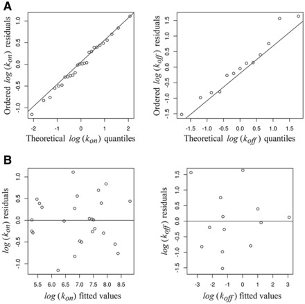
Normal Q–Q plot of the residuals (A) and residuals versus fitted values (B) for model (5) for $\log (k_{\text{on}})$ (left panel) and model (8) for $\log (k_{\text{off}})$ (right panel)

3.4 Predicting ligand rate constants for k_on and k_off

Because the functions of the trHbs mainly depend on the rate at which they uptake and release oxygen, and considering that those rates are unknown for most of the members, it would be important to predict both k_on and k_off for all the trHb family members. For some trHbs, which can be used as leading cases, tentative but well-based functional assignment is available considering their key structural and physicochemical characteristics. Taking Mt-trHbN as an example, this protein’s likely function is to detoxify NO through its oxidation to nitrate by the oxy heme. To fulfill this task, a high oxygen stabilization is required, and the presence of multiple tunnels with a high k_on is likely an important factor (Bidon-Chanal et al., 2006; Lama et al., 2009; Mishra and Meuwly, 2010; Ouellet et al., 2008).

We propose two ways to predict these kinetic rate constants. The first approach, which we call physical-chemically driven, uses the Eyring equation with the theoretically proposed coefficients; the second approach, which we call statistically driven, does not account for the theoretically proposed coefficients, rather it is just a linear model in logarithmic scale of the data and uses the best-fit coefficients without restrictions. We point out that those best-fit coefficients are written in terms of RT to facilitate comparison with the coefficients in the physical-chemically driven approach.

In the case of k_on, specifically, the physical-chemically driven equation takes the theoretically proposed values of β₀ and β₁ (${\beta }_0=\log (k_{\text{B}}T/h)$ and ${\beta }_1=-1$) and takes the value of β₂ that gives rise to the smallest residuals, once β₀ and β₁ are fixed. Namely, by minimizing ${\sum }_{i=1}^n(\log (k_{\text{on}}{)}_i-[\log (k_{\text{B}}T/h)-(1/RT)·\log (e)·\Delta {\text{G}}_{{\text{in}}_i}^{‡}+({\beta }_2/RT)·\log (e)·n_{{\text{HB}}_i}]{)}^2$, we find that ${\beta }_2=-2.95$. Therefore, the first approach to predict k_on is:

$$k_{\text{on}}\text{chem}=\frac{k_{\text{B}}T}{h}·e^{-\frac{\Delta {\text{G}}_{\text{in}}^{‡}}{RT}}·e^{-\frac{2.95·n_{\text{HB}}}{RT}}$$ (9)

The second approach, as explained above, is purely data oriented, and ignores prior knowledge of the relevant physical–chemical constants, using only the best-fit coefficients (Table 1):

$$k_{\text{on}}\text{stat}={10}^{11.81}·e^{-\frac{1.25·\Delta {\text{G}}_{\text{in}}^{‡}}{RT}}·e^{-\frac{1.99·n_{\text{HB}}}{RT}}.$$ (10)

In both approaches, the proposed values for ΔG_HB, 2.95 and 1.99, are in the range of those previously published in the literature. Figure 3 depicts the accuracy of both predictive approaches, $\log (k_{\text{on}}\text{chem})$ and $\log (k_{\text{on}}\text{stat})$, showing their ability to correctly assign the order of the experimental association rate constants. See Supplementary Table S1 to compare predicted with experimental values.

Fig. 3.

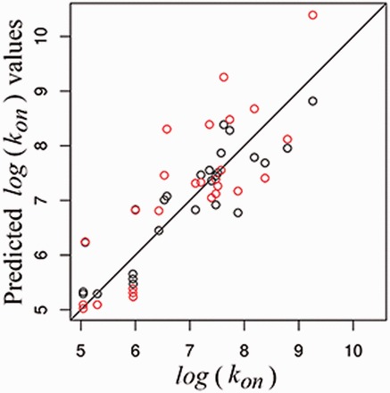
Plot of $\log (k_{\text{on}})$ experimental values versus $\log (k_{\text{on}}\text{chem})$ and $\log (k_{\text{on}}\text{stat})$, in red and black, respectively, with the identity line (Color version of this figure is available at Bioinformatics online.)

Both approaches result in comparatively similar predictions; we note that predicted kinetic constants do not differ from the experimentally reported values by more than an order of magnitude regardless of the approach used. Similar to the case of k_on, we propose two approaches for predicting k_off values. The physical–chemical approach, denoted k_off chem:

$$k_{\text{off}}\text{chem}=e^{-\frac{\Delta \Delta E_{{\text{O}}_2}}{RT}}$$ (11)

and the statistically driven approach, denoted k_off stat:

$$k_{\text{off}}\text{stat}={10}^{-0.04}·e^{-\frac{0.81·\Delta \Delta E_{{\text{O}}_2}}{RT}}$$ (12)

In Figure 4, we plot experimental k_off values versus both k_offchem and k_offstat in a logarithmic scale. Both predictive models were able to correctly assign the order of the predictive experimental constants. See Supplementary Table S2 to compare predicted with experimental values.

Fig. 4.

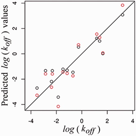
Plot of $\log (k_{\text{off}})$ experimental values versus $\log (k_{\text{off}}\text{chem})$ and $\log (k_{\text{off}}\text{stat})$, in red and black, respectively, with the identity line (Color version of this figure is available at Bioinformatics online.)

4 Discussion

The predictive capacity of our models, together with the statistical evaluation of the individual components included in each model, provides a quantitative context in which we can understand the main factors controlling ligand uptake and release in the trHb family. Whereas internal tunnels and water molecules in the active site modulate ligand entry, the nature of the active site residues controls the kinetics of oxygen release (Fig. 5). The coordination process (k_bond) accounts for the O₂–FeII binding process once oxygen is already in the active site with no surrounding water molecules. Considering that we use the same ligand in any case and taking into account that this process was shown to occur very fast, it was not considered in our model (depicted in red in Fig. 5) (Franzen, 2002; Strickland and Harvey, 2007). In the same line, our statistical analysis shows that O₂ migration to the solvent after the O₂–FeII bond breaking ($\Delta {\text{G}}_{\text{out}}^{‡}$) is not relevant to explain k_off (Fig. 5). In this sense, the results along the variability of the active site show a high correlation, where the more stabilized the O₂, the lower the k_off measured. For example, in the case of the wt form of Mt-trHbN, the key structural position at the active site labeled as B10, occupied by a Tyr, is one of the major responsible residues for its k_off; when this amino acid is mutated to Ala, the k_off increases substantially, because the coordinated oxygen is strongly destabilized. The same trend can be observed for many cases of key amino acids, including wt Mb versus its mutant form where the well-known HisE7 is mutated to Gly, going from a k_off value of 15–1600 s⁻¹. For a deeper analysis of the conservation and variability of the active sites along the trHb family members, see Bustamante et al. (2016).

Fig. 5.

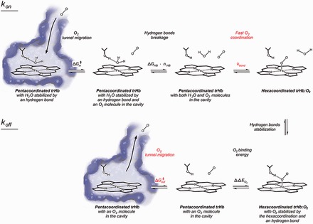
Step-by-step schematic of oxygen uptake and release in trHbs, highlighting the steps considered in our final models. Two steps not involved in the kinetic rate constants are shown in red, either for our statistical analysis (ΔG^‡_out) or for previous evidence (k_bond) (Color version of this figure is available at Bioinformatics online.)

Regarding the role of the internal tunnels, a clear example can be observed comparing the wt and a single mutant form of Mt-trHbN, where the mutation of a Val to a Phe at the structural position G8 promotes a 10 times decrease in k_on. It is important to note that these two proteins have the same active site amino acids, except for the G8 position that does not alter the water molecules, so the only difference accounting for the k_on is the internal tunnel contribution. In this case, the O₂ needs to overcome a higher barrier along the tunnel to reach the active site, mainly due to the size increase of the G8 amino acid, which is reflected in a higher $\Delta {\text{G}}_{\text{in}}^{‡}$ and consecutively in a lower k_on. For a comparison of all herein cases, see Supplementary Tables S1 and S2.

Overall, the varying capacity of main factors to modulate ligand entry and escape translates to diverse biological functions for these hemeproteins. For example, hemeproteins with fast oxygen uptake (high k_on) and fast release (high k_off) are generally oxygen transporters (e.g. Hb and Mb); whereas those with fast uptake (high k_on) and slow release (low k_off) generally undergo multiple ligand reactivity, since oxygen has to enter quickly and stays inside until the second ligand enters to react (e.g. trHbN from M.tuberculosis). It is interesting to note that both entry and exit processes depend on active site interactions, amino acids with positive charge density regions in the active site can both delay oxygen entry by retaining water molecules, and also delay oxygen exit by stabilizing the coordinated oxygen.

Our models suggest therefore, that the only way a protein can control ligand entry without modifying ligand exit is by modifying heme accessibility through tunnels or gates. Note that our model for k_on does not account for internal hexacoordination phenomena, which involves an active site amino acid occupying the sixth coordination position of the iron center. Hence, our model describes the k_on of pentacoordinated trHbs or the k_on of the pentacoordinated state of a hexacoordinated trHb.

Notice that the error values, ϵ_i, in models (5), (7) and (8) include the error inherent in the model as well as in the experimental measurements. For both k_on (model (5)) and k_off (models (7) and (8)), the error was of the same order of magnitude as the variance among the experimental rate constants reported independently in the literature by different groups and techniques. This result strongly supports the absence of any significant theoretical misconceptions in the construction of the models themselves.

A special consideration should be given to the R² value, which, although is a good indicator of the goodness of fit of the corresponding model, it does not suffice to judge its accuracy. A clear example of this problem is found in our analysis of the dissociation rate constants, k_off. The R² values for models (7) and (8) are both reasonably high and nearly indistinguishable (0.787 and 0.784, respectively), even though one of the variables used in model (7) does not make a significant contribution to $\log (k_{\text{off}})$. Based on the R² values alone, both models could be interpreted as being equally accurate, however by further analyzing the P-values and correlation of the variables used in the models we could conclude that the reduced model (8) is more accurate than model (7).

Making extrapolations to the rest of the trHb members (∼1100) is risky considering that we do not yet have evidence about the behavior of the process among the rest of the family members. However, since our analysis was made for mutant proteins that were mostly designed to explore the widest range of k_on and k_off values, and considering that the family of proteins does share a common fold and relevant residues, it is possible to predict k_on and k_off for the other members of the family as well. We proposed two approaches and discussed their pros and cons. The theoretically driven approach uses prior physical–chemical knowledge, therefore it is not strictly limited to a specific subset of proteins; although its coefficients are not the best possible for the available data. The statistically driven approach, which uses the best fitting values of the available data, is strongly related to this small subset of available proteins. In any case, both predictions seem to be very similar for the available data to date, they do not differ by more than one order of magnitude.

5 Conclusion

By performing a rigorous statistical analysis we establish the key factors that control ligand uptake and release in all the studied trHbs. We found that internal tunnels as well as the distal site water molecules control ligand uptake, whereas oxygen stabilization by distal site residues controls ligand release. We also proposed two quantitative approaches to predict k_on and k_off, within an order of magnitude, for the rest of the (around 1100) trHb family members.

Funding

This work was supported by CONICET [PIP 11220110100742] and ANPCYT PICT 2011-1266. L.B. thanks the Pew Fellows grant. J.P.B. holds a CONICET PhD fellowship. M.S., D.A.E., M.A.M. and L.B. are members of CONICET. The funders had no role in study design, data collection and analysis, decision to publish, or preparation of the manuscript.

Conflict of Interest: none declared.

References

- Bidon-Chanal A. et al. (2006) Ligand-induced dynamical regulation of NO conversion in Mycobacterium tuberculosis truncated hemoglobin-N. Proteins, 64, 457–464. [DOI] [PubMed] [Google Scholar]
- Boechi L. et al. (2008) Structural determinants of ligand migration in Mycobacterium tuberculosis truncated hemoglobin O. Proteins, 73, 372–379. [DOI] [PubMed] [Google Scholar]
- Bonamore A. et al. (2005) A novel thermostable hemoglobin from the actinobacterium Thermobifida fusca. FEBS J., 272, 4189–4201. [DOI] [PubMed] [Google Scholar]
- Boron I. et al. (2015) Ligand uptake in Mycobacterium tuberculosis truncated hemoglobins is controlled by both internal tunnels and active site water molecules. F1000Res., 4, 22. [DOI] [PMC free article] [PubMed] [Google Scholar]
- Brunori M. (2000) Structural dynamics of myoglobin. Biophys. Chem., 86, 221–230. [DOI] [PubMed] [Google Scholar]
- Brunori M. et al. (2000) The role of cavities in protein dynamics: crystal structure of a photolytic intermediate of a mutant myoglobin. Proc. Natl Acad. Sci. U. S. A., 97, 2058–2063. [DOI] [PMC free article] [PubMed] [Google Scholar]
- Bustamante J.P. et al. (2014) Ligand uptake modulation by internal water molecules and hydrophobic cavities in hemoglobins. J. Phys. Chem. B, 118, 1234–1245. [DOI] [PubMed] [Google Scholar]
- Bustamante J.P. et al. (2016) Evolutionary and functional relationships in the truncated hemoglobin family. PLoS Comp. Biol., 12, e1004701. [DOI] [PMC free article] [PubMed] [Google Scholar]
- Capece L. et al. (2013) Small ligand-globin interactions: reviewing lessons derived from computer simulation.Biochim. Biophys. Acta., 1834, 1722–1738. [DOI] [PubMed] [Google Scholar]
- Cazade P.A., Meuwly M. (2012) Oxygen migration pathways in NO-bound truncated hemoglobin. Chem. Phys. Chem., 13, 4276–4286. [DOI] [PubMed] [Google Scholar]
- Chodera J. et al. (2011) Alchemical free energy methods for drug discovery: progress and challenges. Curr. Opin. Struct. Biol., 21, 150–160. [DOI] [PMC free article] [PubMed] [Google Scholar]
- Cohen J. et al. (2006) Imaging the migration pathways for O2, CO, NO, and Xe inside myoglobin. Biophys. J., 91, 1844–1857. [DOI] [PMC free article] [PubMed] [Google Scholar]
- Cohen J. et al. (2008) Finding gas migration pathways in proteins using implicit ligand sampling. Methods Enzymol., 437, 439–457. [DOI] [PubMed] [Google Scholar]
- Couture M. et al. (1999) A cooperative oxygen-binding hemoglobin from Mycobacterium tuberculosis. Proc. Natl Acad. Sci. U. S. A., 96, 11223–11228. [DOI] [PMC free article] [PubMed] [Google Scholar]
- Couture M. et al. (2000) Structural investigations of the hemoglobin of the cyanobacterium Synechocystis PCC6803 reveal a unique distal heme pocket. Eur. J. Biochem., 267, 4770–4780. [DOI] [PubMed] [Google Scholar]
- Das T. et al. (2000) Ligand binding in the ferric and ferrous states of paramecium hemoglobin. Biochemistry, 39, 14330–14340. [DOI] [PubMed] [Google Scholar]
- Dinner A. et al. (2000) Understanding protein folding via free-energy surfaces from theory and experiment. Trends Biochem. Sci., 25, 331–339. [DOI] [PubMed] [Google Scholar]
- Elber R. (2010) Ligand diffusion in globins: simulations versus experiment. Curr. Opin. Struct. Biol., 20, 162–167. [DOI] [PMC free article] [PubMed] [Google Scholar]
- Forti F. et al. (2011) Ligand migration in Methanosarcina acetivorans protoglobin: effects of ligand binding and Dimeric assembly. J. Phys. Chem. B, 115, 13771–13780. [DOI] [PubMed] [Google Scholar]
- Franzen S. (2002) Spin-dependent mechanism for diatomic ligand binding to heme. Proc. Natl Acad. Sci. U. S. A., 99, 16754–16759. [DOI] [PMC free article] [PubMed] [Google Scholar]
- Giangiacomo L. et al. (2005) The truncated oxygen-avid hemoglobin from Bacillus subtilis: x-ray structure and ligand binding properties. J. Biol. Chem., 280, 9192–9202. [DOI] [PubMed] [Google Scholar]
- Giordano D. et al. (2011) Ligand and proton-linked conformational changes of the ferrous 2/2 hemoglobin of Pseudoalteromonas haloplanktis TAC125. IUBMB Life, 63, 566–573. [DOI] [PubMed] [Google Scholar]
- Giordano D. et al. (2015) Structural flexibility of the heme cavity in the cold-adapted truncated hemoglobin from the Antarctic marine bacterium Pseudoalteromas haloplanktis TAC125. FEBS J. 282, 2948–2965. [DOI] [PubMed] [Google Scholar]
- Goldbeck R. et al. (2006) Water and ligand entry in myoglobin: assessing the speed and extent of heme pocket hydration after CO photodissociation. Proc. Natl Acad. Sci. U. S. A., 103, 1254–1259. [DOI] [PMC free article] [PubMed] [Google Scholar]
- Guallar V. et al. (2009) Ligand migration in the truncated hemoglobin-II from Mycobacterium tuberculosis: the role of G8 tryptophan. J. Biol. Chem., 284, 3106–3116. [DOI] [PMC free article] [PubMed] [Google Scholar]
- Hoy J.A. et al. (2004) The crystal structure of synechocystis hemoglobin with a covalent heme linkage. J. Biol. Chem., 279, 16535–16542. [DOI] [PubMed] [Google Scholar]
- Ilari A. et al. (2007) Crystal structure and ligand binding properties of the truncated hemoglobin from Geobacillus stearothermophilus. Arch. Biochem. Biophys., 457, 85–94. [DOI] [PubMed] [Google Scholar]
- Kepp K.P. (2013) O2 binding to heme is strongly facilitated by near-degeneracy of electronic states. ChemPhysChem, 14, 3551–3558. [DOI] [PubMed] [Google Scholar]
- Kutner M. et al. (2005). Applied Linear Statistical Models. 5th edn McGraw Hill, Irwin. [Google Scholar]
- Lama A. et al. (2009) Role of pre-A motif in nitric oxide scavenging by truncated hemoglobin, HbN, of Mycobacterium tuberculosis. J. Biol. Chem., 284, 14457–14468. [DOI] [PMC free article] [PubMed] [Google Scholar]
- Laverman L., Ford P. (2001) Mechanistic studies of nitric oxide reactions with water soluble iron(II), cobalt(II), and iron(III) porphyrin complexes in aqueous solutions: implications for biological activity. J. Am. Chem. Soc., 123, 11614–11622. [DOI] [PubMed] [Google Scholar]
- Laverman L. et al. (1997) A dissociative mechanism for reactions of nitric oxide with water soluble iron(III) porphyrins. J. Am. Chem. Soc., 119, 12663–12664. [Google Scholar]
- Lu C. et al. (2007) Structural and functional properties of a truncated hemoglobin from a food-borne pathogen Campylobacter jejuni. J. Biol. Chem., 282, 13627–13636. [DOI] [PubMed] [Google Scholar]
- Marcelli A. et al. (2012) Following ligand migration pathways from picoseconds to milliseconds in type II truncated hemoglobin from Thermobifida fusca. PLoS One, 7, e39884. [DOI] [PMC free article] [PubMed] [Google Scholar]
- Markovitch O., Agmon N. (2007) Structure and energetics of the hydronium hydration shells. J. Phys. Chem. A, 111, 2253–2256. [DOI] [PubMed] [Google Scholar]
- Marti M.A. et al. (2006) Dioxygen affinity in heme proteins investigated by computer simulation. J. Inorg. Biochem., 100, 761–770. [DOI] [PubMed] [Google Scholar]
- Milani M. et al. (2001) Mycobacterium tuberculosis hemoglobin N displays a protein tunnel suited for O2 diffusion to the heme. EMBO J., 20, 3902–3909. [DOI] [PMC free article] [PubMed] [Google Scholar]
- Milani M. et al. (2003) A TyrCD1/TrpG8 hydrogen bond network and a TyrB10–TyrCD1 covalent link shape the heme distal site of Mycobacterium tuberculosis hemoglobin O. Proc. Natl Acad. Sci. U. S. A., 100, 5766–5771. [DOI] [PMC free article] [PubMed] [Google Scholar]
- Milani M. et al. (2004) Heme-ligand tunneling in group I truncated hemoglobins. J. of Biol. Chem., 279, 21520–21525. [DOI] [PubMed] [Google Scholar]
- Mishra S., Meuwly M. (2009) Nitric oxide dynamics in truncated hemoglobin: docking sites, migration pathways, and vibrational spectroscopy from molecular dynamics simulations. Biophys. J., 96, 2105–2118. [DOI] [PMC free article] [PubMed] [Google Scholar]
- Mishra S., Meuwly M. (2010) Atomistic simulation of NO dioxygenation in group I truncated hemoglobin. J. Am. Chem. Soc., 132, 2968–2982. [DOI] [PubMed] [Google Scholar]
- Nardini M. et al. (2006) Structural determinants in the group III truncated hemoglobin from Campylobacter jejuni. J. Biol. Chem., 281, 37803–37812. [DOI] [PubMed] [Google Scholar]
- Oliveira A.S.F. et al. (2014) Exploring O2 diffusion in A-type cytochrome c oxidases: molecular dynamics simulations uncover two alternative channels towards the binuclear site. PLoS Comput. Biol., 10, e1004010. [DOI] [PMC free article] [PubMed] [Google Scholar]
- Olson J., Phillips G. (1997) Myoglobin discriminates between O2, NO, and CO by electrostatic interactions with the bound ligand. J. Biol. Inorg. Chem., 2, 544–552. [Google Scholar]
- Ouellet H. et al. (2003) Reactions of Mycobacterium tuberculosis truncated hemoglobin O with ligands reveal a novel ligand-inclusive hydrogen bond network. Biochemistry, 42, 5764–5774. [DOI] [PubMed] [Google Scholar]
- Ouellet H. et al. (2007a) Reaction of Mycobacterium tuberculosis truncated hemoglobin O with hydrogen peroxide: evidence for peroxidatic activity and formation of protein-based radicals. J. Biol. Chem., 282, 7491–7503. [DOI] [PubMed] [Google Scholar]
- Ouellet H. et al. (2007b) The roles of Tyr(CD1) and Trp(G8) in Mycobacterium tuberculosis truncated hemoglobin O in ligand binding and on the heme distal site architecture. Biochemistry, 46, 11440–11450. [DOI] [PubMed] [Google Scholar]
- Ouellet Y. et al. (2006) Ligand interactions in the distal heme pocket of Mycobacterium tuberculosis truncated hemoglobin N: roles of TyrB10 and GlnE11 residues. Biochemistry, 45, 8770–8781. [DOI] [PubMed] [Google Scholar]
- Ouellet Y.H. et al. (2008) Ligand binding to truncated hemoglobin N from Mycobacterium tuberculosis is strongly modulated by the interplay between the distal heme pocket residues and internal water. J. Biol. Chem., 283, 27270–27278. [DOI] [PMC free article] [PubMed] [Google Scholar]
- Pearlman D.A. et al. (1995) AMBER, a package of computer programs for applying molecular mechanics, normal mode analysis, molecular dynamics and free energy calculations to simulate the structural and energetic properties of molecules. Comput. Phys. Commun., 91, 1–41. [Google Scholar]
- Perilla J. et al. (2015) Molecular dynamics simulations of large macromolecular complexes. Curr. Opin. Struct. Biol., 31, 64–74. [DOI] [PMC free article] [PubMed] [Google Scholar]
- Perutz M.F., Mathews F.S. (1966) An x-ray study of azide methaemoglobin. J. Mol. Biol., 21, 199–202. [DOI] [PubMed] [Google Scholar]
- Pesce A. et al. (2000) A novel two-over-two α-helical sandwich fold is characteristic of the truncated hemoglobin family. EMBO J., 19, 2424–2434. [DOI] [PMC free article] [PubMed] [Google Scholar]
- Pesce A. et al. (2011) Structural characterization of a group II 2/2 hemoglobin from the plant pathogen Agrobacterium tumefaciens. Biochimica Et Biophysica Acta - Proteins and Proteomics, 1814, 810–816. [DOI] [PubMed] [Google Scholar]
- Potapov V. et al. (2015) Data-driven prediction and design of bZIP coiled-coil interactions. PLoS Comput. Biol., 11, e1004046. [DOI] [PMC free article] [PubMed] [Google Scholar]
- Pucci F., Rooman M. (2014) Stability curve prediction of homologous proteins using temperature-dependent statistical potentials. PLoS Comput. Biol., 10, e1003689. [DOI] [PMC free article] [PubMed] [Google Scholar]
- R Core Team (2013). R: A language and environment for statistical computing. R Foundation for Statistical Computing, Vienna, Austria. ISBN 3-900051-07-0.
- Scherlis D. et al. (2007) Simulation of heme using DFT + U: a step toward accurate spin-state energetics. J. Phys. Chem. B, 111, 7384–7391. [DOI] [PubMed] [Google Scholar]
- Scott E.E. et al. (2001) Mapping the pathways for O2 entry into and exit from myoglobin. J. Biol. Chem., 276, 5177–5188. [DOI] [PubMed] [Google Scholar]
- Silk D. et al. (2014) Model selection in systems biology depends on experimental design. PLoS Comput. Biol., 10, e1003650. [DOI] [PMC free article] [PubMed] [Google Scholar]
- Sotomayor M., Schulten K. (2007) Single-molecule experiments in vitro and in silico. Science, 316, 1144–1148. [DOI] [PubMed] [Google Scholar]
- Strickland N., Harvey J.N. (2007) Spin-forbidden ligand binding to the ferrous-heme group: ab initio and DFT studies. J. Phys. Chem. B, 111, 841–852. [DOI] [PubMed] [Google Scholar]
- Watts R. et al. (2001) A hemoglobin from plants homologous to truncated hemoglobins of microorganisms. Proc. Natl. Acad. Sci. U. S. A., 98, 10119–10124. [DOI] [PMC free article] [PubMed] [Google Scholar]
- Wilk M.B., Gnanadesikan R. (1968) Probability plotting methods for the analysis of data. Biometrika (Biometrika Trust), 55, 1–17. [PubMed] [Google Scholar]
- Wittenberg J.B. et al. (2002) Truncated hemoglobins: a new family of hemoglobins widely distributed in bacteria, unicellular eukaryotes, and plants. J. Biol. Chem., 277, 871–874. [DOI] [PubMed] [Google Scholar]
- Yang F., Phillips G.N., Jr., (1996) Crystal structures of CO-, deoxy- and met-myoglobins at various pH values. J. Mol. Biol., 256, 762–774. [DOI] [PubMed] [Google Scholar]
Associated Data
This section collects any data citations, data availability statements, or supplementary materials included in this article.