Assortative mating on complex traits revisited: double first cousins and the X-chromosome

Abstract

Mate choice through direct assortment on heritable traits, assortative mating (AM), is predicted in theory to inflate the genetic variance in a population and the correlation between relatives. Here, we revisit the theory of AM, first established in the landmark 1918 paper from RA Fisher, and provide new theory and analytical results. In particular, we shed light on inconsistencies in the literature regarding the correlation between double first cousins under AM and provide a solution. We derive new theory for AM due to X-chromosome loci. We show in the latter case that the inflation of genetic variance induced under AM is twice as large in females compared to males. These two theoretical contributions are verified and illustrated through simulations. We also provide a more general unified framework for the correlation between relatives in a non-inbred population.

Assortative mating (AM), that is preference for mates with similar phenotypes, is commonly observed in multiple sexually reproducing species [8]. Seminal works from [5] and [19] have laid the theoretical foundation of the genetic consequences of AM. Despite using different analytical approaches, [5] and [19] established that AM on a particular trait, compared to random mating (RM), modifies the genetic variance of that trait in the population as well as the resemblance between relatives with respect to that particular trait. [19] also highlighted that AM induces an increase in homozygosity at causal loci of the trait driving the assortment. However, the magnitude of homozygosity thus induced decreases with the number of causal loci, and is almost negligible if the number of causal loci is large.

Results on the effect of AM from [5] were sometimes given without rigorous theoretical proofs. For example, [5] predicted that the correlation between parents and offspring or between siblings would not be affected by linkage. The proof of this result was only established 60 years later by [11], although [4] had previously generalized the change in genetic variance due to AM to an arbitrary number of loci and an arbitrary genetic map. The generalization to an arbitrary number of loci and an arbitrary genetic map proposed in [4] was achieved by the introduction of an effective number of loci M_e (Eq. 4.8.13 in [4]), which equals the actual number M of causal loci when there is free recombination and when all causal variants contribute equally to the genetic variance; otherwise M_e < M. Similar to [19], [4] predict the increase of homozygosity at causal loci of the trait driving the assortment to be inversely proportional to M_e and therefore conclusions from [4] are consistent with [19] in that homozygosity is negligible when the (effective) number of loci is large. [7, 6] made a substantial contribution in formalizing the consequences of AM on the correlation between relatives for a broader class of pedigree relationships (including non-traditional relationships such as step sibs, and including inbred individuals) than considered by its predecessors. Other contributions are from [2], who considered AM on traits controlled by infinitely many loci in the presence of dominance; and [9], who present a comprehensive overview and synthesis of all these results.

Despite these outstanding contributions, a number of areas of the theory of the genetic consequences of AM remain unclear. First, although predictions from [5] to [9] are consistent for most common pedigree relationships, no consensus can be found on the consequence of AM on the resemblance between double first cousins (DFC), for which there are a number of different results reported in the literature ([5, 7]). Secondly, despite evidence of mate preference being controlled by sex-linked variants ([16, 13], most theoretical predictions of the consequence of AM on the genetic variance in the population mostly concentrate on autosomal variants. An exception is [14], who predicted, following the same analytical framework as [11], the correlation between relatives when mates assort on a trait controlled by autosomal and X-linked loci.

Here, we address these two questions through theory and simulations. In particular, we assess through simulations the accuracy of different theoretical predictions of the correlation between DFC under AM. In addition, we extend existing theory for infinitesimal and finite locus models in the case when the trait on which AM occurs is wholly caused by genes on the sex chromosomes rather than on autosomes. In this study we assume that assortment is primarily on phenotype, that there is no sexual selection (i.e. both sexes have equal opportunity to reproduce), that all covariance between relatives is genetic, that all genetic variation is additive and that there is no inbreeding.

Review of consensus results

Variance under equilibrium

We assume that AM occurs on a trait controlled by a large number (n) of variants and thus additive (breeding) genetic values can be assumed normally distributed. The assumption of a large number of variants is supported by overwhelming evidence that complex traits in humans (and other species) are highly polygenic ([18]). We therefore follow the derivations of [2], which are a based on normal distribution assumptions. At generation t, we denote A_t as the additive genetic value and E as the environmental value. We allow the variance of A_t to vary over time but that of E to be constant over time. We define $h_t^2=\mathrm{var}\left(A_t\right)/\left[\mathrm{var}\left(A_t\right)+\mathrm{var}(E)\right]$, with var(E) the environmental variance. When not using any subscript, h² simply denotes the heritability in the base population, i.e. under RM. For notation, we use A_M and A_F to denote autosomal male and female breeding values of mates and Y_M and Y_F the phenotypic value of males and females respectively. From [2],

$$\begin{gathered} A_{F(t)}=h_t^2{Y}_{F(t)}+r_{F(t)} \\ {A}_{M(t)}=h_t^2{Y}_{M(t)}+r_{M(t)}.3 \end{gathered}$$ (1)

In equation (1), r_F(t) and r_M(t) are normally distributed residual errors with mean 0 and variances $\mathrm{var}\left(r_{F(t)}\right)=\mathrm{var}\left(A_{F(t)}\right)\left[1-h_t^2\right]$ and $\mathrm{var}\left(r_{M(t)}\right)=\mathrm{var}\left(A_{M(t)}\right)\left[1-h_t^2\right]$.

Per definition, var(Y_t) = var(A_t)+var(E), and assuming that male and female phenotypic variances are the same, it follows that cov (Y_F(t), Y_M(t)) = ρvar(Y_F(t)) = ρvar(Y_M(t)), where ρ is the phenotypic correlation between mates, which is assumed to be constant over generations.

Using equation (1),

$$\mathrm{cov}\left(A_{F(t)},A_{M(t)}\right)=\rho h_t^4\mathrm{var}\left(Y_t\right)=\rho h_t^2\mathrm{var}\left(A_t\right),$$ (2)

so that the correlation between the additive genetic values of the mates is the well-known result $\rho h_t^2$ ([19]).

The recurrence equation for the additive genetic variance is derived from the infinitesimal model ([5, 1]) as,

$$A_{t+1}=\frac{1}{2}{A}_{F(t)}+\frac{1}{2}{A}_{M(t)}+m,$$ (3)

with m a segregation term that has constant variance var(m) = var(A₀)/2, where var(A₀) is the additive genetic variance in the base population, i.e. the additive genetic variance under random mating. From equation (1) to (3),

$$\mathrm{var}\left(A_{t+1}\right)=\frac{1}{2}\mathrm{var}\left(A_t\right)\left[1+\rho h_t^2\right]+\frac{1}{2}\mathrm{var}\left(A_0\right).$$ (4)

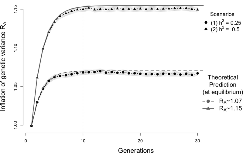
At equilibrium, which is generally reached within few generations (Figure 2), this gives the well-known result ([19, 2, 9]) of

$$\frac{\mathrm{var}\left(A_{eq}\right)}{\mathrm{var}\left(A_0\right)}=\frac{1}{1-\rho h_{eq}^2},$$ (5)

where var(A_eq) and $h_{eq}^2$ respectively denote the additive genetic variance and heritability in the equilibrium population. Equation (5) can also be expressed (as in [9], eq. 7.19b) in terms of base population parameters, i.e.

$$\mathrm{var}\left(A_{eq}\right)/\mathrm{var}\left(A_0\right)=\frac{2+\left[\sqrt{1-4\rho h^2\left(1-h^2\right)}-1\right]/h^2}{2(1-\rho )}=R_A,$$ (6)

which to first order approximation, when |ρh²| ≪ 1, becomes

$$\mathrm{var}\left(A_{eq}\right)/\mathrm{var}\left(A_0\right)\approx 1+\rho h^2/(1-\rho ).$$ (7)

Figure 2:

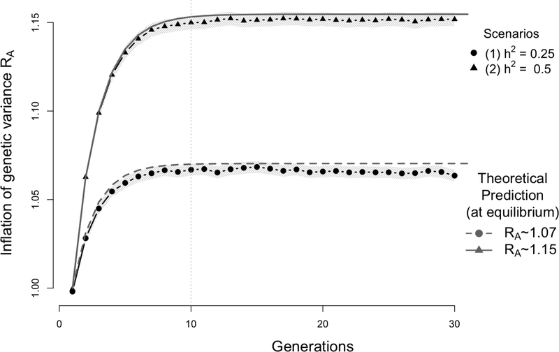
Simulation results showing the inflation of the genetic variance (with 95% confidence interval - light band around each dot) induced by assortative mating (AM) on a quantitative trait controlled by unlinked autosomal variants. Data were simulated assuming that the trait driving assortment is controlled by 1,000 independent bi-allelic variants with allele frequency p = 0.5. Two scenarios were considered with either a heritability (1) h² = 0.25 or (2) h² = 0.5. Each simulation replicate generates a population of 2,500 males and 2,500 females undergoing AM for 30 generations with a mate correlation ρ = 0.25. The empirical genetic variance is calculated at each iteration as the sampling variance (over the 5,000 generated individuals) of the simulated breeding value. The ratio of the empirical genetic variance over the genetic variance in the base population was averaged over 1,000 simulation replicates (i.e. each dot is the average over 1,000 simulated populations) and compared with theoretical expectation R_A from equation (6). In the first scenario (h² = 0.25, lower dotted curve) R_A ∼ 1.07 and in the second scenario (h² = 0.5, upper plain curve), R_A ∼ 1.15.

Finally, ratio of heritabilities, as previously reported by [12], can be expressed as

$$h_{eq}^2/h^2=\frac{1}{1-\rho h_{eq}^2\left(1-h^2\right)}=\frac{R_A}{1+h^2\left(R_A-1\right)}.$$ (8)

Resemblance between relatives

As shown in Table 3 from [3], results from [5] and [19] regarding the correlation between relatives are consistent for unilineal relatives and for descendants of half- and full-sibs. They assume, for a large number of loci, multivariate normality of phenotypes and breeding values between pairs of relatives and large effective population size so that inbreeding can be ignored. In addition, they assume homogeneity of variance, in that the variance in breeding values is the same in different families.

If ρ is the phenotypic correlation between mates and ${\rho }_a=\rho h_{eq}^2$ is the correlation of breeding values between mates at equilibrium, then the results from [5], [19], [2], [6] and [11] can be summarised as follows.

Unilineal relatives

Let k be the number of meioses between individuals i and j, when i and j have a single common ancestor. The numerator relationship R_ij between i and j, i.e. twice their coancestry coefficient, equals (1/2)^k. Using these notations, we can write the known formula ([5, 11]) for the phenotypic correlation between i and j:

$$\mathrm{corr}\left(Y_i,Y_j\right)=R_{ij}{h}_{eq}^2(1+\rho ){\left(1+{\rho }_a\right)}^{k-1}={(1/2)}^k{h}_{eq}^2(1+\rho ){\left(1+{\rho }_a\right)}^{k-1}.$$ (9)

In particular, if i is j’s great grandfather, then k = 3 and $\mathrm{corr}\left(Y_i,Y_j\right)=\frac{1}{8}{h}_{eq}^2(1+\rho ){\left(1+{\rho }_a\right)}^2$ as previously reported in [3] for example.

Descendants of fullsibs

From [5], the correlation between fullsibs i and j can be expressed as

$$\mathrm{corr}\left(Y_i,Y_j\right)=\frac{1}{2}{h}_{eq}^2\left(1+{\rho }_a\right).$$ (10)

We now propose to extend this relationship to the case of descendants of fullsibs. [6] introduced a general linear model for the covariance between relatives, that predicts the correlation between descendants of fullsbibs to be attenuated by a factor (1 + ρ_a) at each generation. Consequently, if individual i is k₁ generations from the first fullsib and individual j is k₂ generations from the second fullsib, then R_ij = (1/2)^k, with k = k₁ + k₂ + 1 and

$$\mathrm{corr}(Y_i,Y_j)={(1/2)}^k{h}_{eq}^2{(1+{\rho }_a)}^k.$$ (11)

Note that when k₁ = k₂ = 0, we find the same result as in equation (10). Also when k₁ = 0 and k₂ = 1, which corresponds to avuncular relationships (niece/nephew versus aunt/uncle), we find the known relationship from [5] and [3]: $\mathrm{corr}\left(Y_i,Y_j\right)=\frac{1}{4}{h}_{eq}^2{\left(1+{\rho }_a\right)}^2$.

Descendants of halfsibs

This relation was not studied by [5]. Starting from the correlation between halfsibs i and j ([11]),

$$\mathrm{corr}\left(Y_i,Y_j\right)=\frac{1}{4}{h}_{eq}^2\left(1+2{\rho }_a+\rho {\rho }_a\right),$$ (12)

and applying the same linearity principle ([6]) as before, we can extend equation (12) to the case of descendants of halfsibs. Let us assume that individual i is k₁ generations from the first halfsib and individual j is k₂ generations from the second halfsib. The numerator relationship between i and j is in this case is R_ij = (1/2)^k, with k = k₁ +k₂ +2. For example, for halfsibs themselves, k₁ = k₂ = 0. We then derive the extended formula:

$$\mathrm{corr}\left(Y_i,Y_j\right)={(1/2)}^k{h}_{eq}^2\left(1+2{\rho }_a+\rho {\rho }_a\right){\left(1+{\rho }_a\right)}^{k-2}$$ (13)

Generalization

All expressions above have a similar form, with a term depending on one or two matings in the pedigree of individuals i and j, and a term depending on the number of generations since those matings. A general equation for the aforementioned relationships therefore has the form,

$$\mathrm{corr}\left(Y_i,Y_j\right)={(1/2)}^k{h}_{eq}^2{C}_{ij}{\left(1+{\rho }_a\right)}^k$$ (14)

with the constant C_ij equal to (1+ρ)/(1+ρ_a) for unilineal relatives, (1+2ρ_a+ρρ_a)/(1+ρ_a)² for descendants of halfsibs and 1 for descendants of fullsibs. For large heritabilities, all these 3 ratios are approximately unity and the most general form is

$$\mathrm{corr}\left(Y_i,Y_j\right)\approx {(1/2)}^k{h}_{eq}^2{\left(1+{\rho }_a\right)}^k$$ (15)

Hence, for this approximation an estimate of $h_{eq}^2$ from corr(Y_i,Y_j)/(1/2)^k is biased upwards by (1+ρ_a)^k ≈ exp(kρ_a).

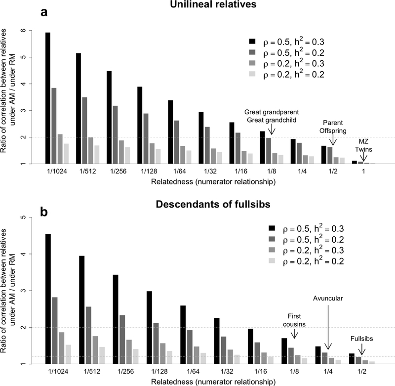
We represent in Figure 1 how AM inflates the correlation between relatives for the three types of relationships described above. Importantly, we illustrate that AM disproportionately inflates the correlation between distant relatives.

Figure 1:

Theoretical ratio of the phenotypic correlation between relatives in a population undergoing assortative mating (AM) relative to a randomly mating (RM) population. Two types of pedigree relationships are considered: unilineal (equation 9) in panel a and descendants of fullsbibs (equation (11) in panel b. Four cases are considered: (ρ = 0.5,h² = 0.3), (ρ = 0.5,h² = 0.2), (ρ = 0.2,h² = 0.3) and (ρ = 0.2,h² = 0.2).

Double first cousins

The case of double first cousins (DFC) is particularly interesting as different formulas are proposed in the literature. [5] first predicted the phenotypic correlation between DFC under AM to be

$$r_{DFC}^{(Fisher)}=\frac{1}{4}{h}_{eq}^2\left(1+3{\rho }_a\right).$$ (16)

Following [5], [11] introduced a new analytical framework to predict a wide range of correlations between relatives under AM but failed to extend his approach to DFC. He wrote : “...the proper enforcement of phenotypic assortative mating at the level of analysis employed here is not obvious, and the additive special case of Fisher’s (1918) result, was not derived”. [7] revisited the question using a different approach which models the 4-dimensional distribution of breeding values of males sibs mating with females sibs. One key insight of [7] was to prove that AM could modify the frequency of certain mating types in the population, like for example those giving rise to DFC. He showed however that AM does not uniformly affect all types of mating in the population. For example, for what he terms as Type 1 relatives, i.e. those connected through only one of their parents (half-sibs, first cousins, etc.), Gimelfarb showed that their frequency in an assortatively mating population is not altered relative to a randomly mating population. For Type 2 relatives, i.e. if both parents of one of them are connected to only one of the parents of the other (e.g. avuncular relationship), Gimelfarb showed that the frequency could be increased in a population undergoing assortative mating. However, he also noted that avuncular was an exception to other Type 2 relationships. DFCs fall in Gimelfarbs third type of relatives (Type 3), where members of the pair of relatives are connected through both their parents. He showed in this case that the probability of observing DFC is larger under AM than under RM. Along with that result, he also demonstrates that the genetic variance in (the population of) DFC is larger under AM than that of the general population. These two conclusions lead to the following formula for the correlation between DFC:

$$r_{DFC}^{(Gimelfarb)}=\frac{\frac{1}{4}{h}_{eq}^2{\left(1+{\rho }_a\right)}^3}{1-\frac{1}{4}{\left(1+{\rho }_a\right)}^2{\rho }_a^2},$$ (17)

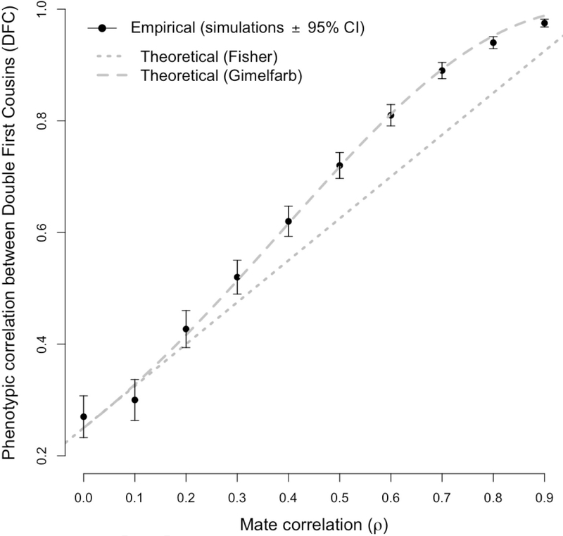
As highlighted in [7], when |ρ_a| ≪ 1 both inflations in the frequency of DFC and in the genetic variance among DFC are negligible, leading thus to Fisher’s result in equation (16). This is illustrated on Figure 4, which shows plots of the mathematical functions of ρ_a described in equations (16) and (17). [7] underlined the discrepancy between equation (17) and a prediction from [2]. In Bulmer’s 1980 edition, the correlation between DFC was given as $r_{DFC}^{(Bulmer)}=0.25{\left(1+{\rho }_a\right)}^2$ but this was removed in the 1985 edition and no explicit equation was given therein. Also, the acknowledgement section of [11] refers to Bulmer’s formula from [2] (1980 edition) as not agreeing with Fisher’s: “With the exception of double first cousins, Dr Bulmers’s correlations agree with Fisher’s”.

Figure 4:

Phenotypic correlation of simulated double first cousins (DFC) as a function of the mate correlation ρ. Each simulation replicate (black dot) corresponds to a simulated population of 1,000 males and 1,000 females undergoing AM for 10,000 generations with a given value of ρ. The heritability is fixed in this simulation to h² = 1. For each value of ρ, the empirical correlation between DFC was calculated across the 10,000 generations and compared to theoretical expectations from Fisher (1918) (equation 16) and Gimelfarb (1981a) (equation 17). CI stands for Confidence Interval.

Another difference between [5] and [7] is that Fisher’s reasoning implies exchangeability between male or female sibs. In other words, each of the female sibs (from one family) is equally likely to mate with each of the male sibs (from another family). Under this assumption, Fisher’s modelling therefore does not account for Mendelian sampling creating differences in breeding values (and phenotypes) between sibs. In contrast, Gimelfarb’s modelling, which does not rely on this assumption, allows asymmetrical correlation between actual mates versus potential mates. In practice, the exchangeability assumption may be too restrictive. For example, if there is AM in the population for a trait like human height therefore, then we can reasonably expect the taller member of a female sib-pair to be more likely to partner with the taller member of a male sib-pair.

We present later a simulation study comparing the predictions from equations (16) and (17) for different values of ρ_a (Figure 4).

Assortative mating on traits of the X-chromosome

We assume a large number of loci so that additive genetic (breeding) values are normally distributed. For notation, we use A_MX and A_FX to denote additive genetic values from the X-chromosomes in males and females, respectively. For male and female offspring we can write their breeding values as functions of their parents’ breeding values:

$$A_{MX(t+1)}=\frac{c}{\sqrt{2}}{A}_{FX(t)}+m_M$$ (18)

$$A_{FX(t+1)}=\frac{1}{2}{A}_{FX(t)}+\frac{1}{c\sqrt{2}}{A}_{MX(t)}+m_F$$ (19)

In equations 18 and 19, c is a constant scaling factor, defined in base population terms, to reflect the difference in male and female genetic variance on the X-chromosome:

$$c=\sqrt{\frac{\mathrm{var}\left[A_{MX(0)}\right]}{\mathrm{var}\left[A_{FX(0)}\right]}}.$$ (20)

Parameter c also reflects the effect of dosage compensation ([9]).

The Mendelian sampling terms m_M and m_F have variances $\mathrm{var}\left(m_M\right)=\frac{1}{2}\mathrm{var}\left(A_{MX(0)}\right)$ and and $\mathrm{var}\left(m_F\right)=\frac{1}{4}\mathrm{var}\left(A_{FX(0)}\right)$. At any generation, the covariance in breeding values between male and female parents is $\rho {\left\{\mathrm{var}\left[A_{MX(t)}\right]\mathrm{var}\left[A_{FX(t)}\right]\right\}}^{1/2}$.

Recurrence equations are,

$$\mathrm{var}\left(A_{MX(t+1)}\right)=\frac{c^2}{2}\mathrm{var}\left(A_{FX(t)}\right)+\frac{1}{2}\mathrm{var}\left(A_{MX(0)}\right)$$ (21)

$$\begin{gathered} \mathrm{var}\left(A_{FX(t+1)}\right)=\frac{1}{4}\mathrm{var}\left(A_{FX(t)}\right)+\frac{1}{2c^2}\mathrm{var}\left(A_{MX(t)}\right)+\frac{\rho {\left\{\mathrm{var}\left[A_{MX(t)}\right]\mathrm{var}\left[A_{FX(t)}\right]\right\}}^{1/2}}{c\sqrt{2}} \\ +\frac{1}{4}\mathrm{var}\left(A_{FX(0)}\right) \end{gathered}$$ (22)

If we denote R_M and R_F as the ratios between equilibrium genetic variances over RM genetic variances in males and females respectively, then these equations can be simplified to,

$$R_M=\frac{1}{2}\left(1+R_F\right)\text{and}{R}_F=1+\rho \sqrt{R_F\left(1+R_F\right)},$$ (23)

which has the solution

$$R_M=1+\frac{\rho \left(3\rho +\sqrt{8+{\rho }^2}\right)}{4\left(1-{\rho }^2\right)}\text{and}{R}_F=1+\frac{2\rho \left(3\rho +\sqrt{8+{\rho }^2}\right)}{4\left(1-{\rho }^2\right)}.$$ (24)

We now add the effect of environmental variance, and assume that environmental variance is the same for males and females. We define X-chromosome heritabilities in males and females as

$$h_{MX(t)}^2=\mathrm{var}\left(A_{MX(t)}\right)/\left[\mathrm{var}\left(A_{MX(t)}\right)+\mathrm{var}(E)\right],$$ (25)

$$h_{FX(t)}^2=\mathrm{var}\left(A_{FX(t)}\right)/\left[\mathrm{var}\left(A_{FX(t)}\right)+\mathrm{var}(E)\right].$$ (26)

Following the same logic as for autosomal breeding values, the covariance in X-chromosome breeding values for male and female parents is,

$$\mathrm{cov}\left(A_{MX(t)},A_{FX(t)}\right)=\rho {\left\{h_{MX(t)}^2{h}_{FX(t)}^2\mathrm{var}\left[A_{MX(t)}\right]\mathrm{var}\left[A_{FX(t)}\right]\right\}}^{1/2}.$$

This is the only change from equation (22), which was for heritabilities of 1. Therefore, at equilibrium,

$$R_M=\frac{1}{2}\left(1+R_F\right)\text{as}\text{before}\text{and}{R}_F=1+\rho \sqrt{h_{MX}^2{h}_{FX}^2{R}_F\left(1+R_F\right),}$$ (27)

which has as solution

$$R_M=1+\frac{\rho \left(3\rho h_{MX}^2{h}_{FX}^2+\sqrt{h_{MX}^2{h}_{FX}^2\left(8+{\rho }^2{h}_{MX}^2{h}_{FX}^2\right)}\right)}{4\left(1-{\rho }^2{h}_{MX}^2{h}_{FX}^2\right)}=1+\lambda ,$$ (28)

and

$$R_F=1+\frac{2\rho \left(3\rho h_{MX}^2{h}_{FX}^2+\sqrt{h_{MX}^2{h}_{FX}^2\left(8+{\rho }^2{h}_{MX}^2{h}_{FX}^2\right)}\right)}{4\left(1-{\rho }^2{h}_{MX}^2{h}_{FX}^2\right)}=1+2\lambda .$$ (29)

We can therefore see from equations (18) and (19) that the inflation of genetic variance is twice as large in females compared to males. One direct consequence of this result is that positive AM is expected to reduce the effect of dosage compensation (parameter c²) in the equilibrium population, by a factor equal to 1−λ/(1+2λ) ≤ 1. For example, under full dosage compensation, the ratio of genetic variance between males and females is c² = 2 in a base population undergoing random mating. This ratio would therefore decrease to ∼ 1.64 (i.e. ∼ 17.8% decrease) under AM if for instance ρ = 0.25, var[A_MX(0)] = 0.5 and var[A_FX(0)] = 0.25.

At equilibrium, equations for the male and female heritability inflation can be written as

$$\frac{h_{MX}^2}{h_{MX(0)}^2}=\frac{R_M}{1+h_{MX(0)}^2\left(R_M-1\right)}\text{and}\frac{h_{FX}^2}{h_{FX(0)}^2}=\frac{R_F}{1+h_{FX(0)}^2\left(R_F-1\right)}.$$ (30)

As for genetic variance, AM also reduces the ratio of heritability between males and females in the equilibrium population as compared to the base population. We express below that reduction factor as

$$\left(\frac{h_{MX}^2}{h_{FX}^2}\right)/\left(\frac{h_{MX(0)}^2}{h_{FX(0)}^2}\right)=\left(\frac{1+\lambda }{1+2\lambda }\right)\left(\frac{1+2\lambda h_{FX(0)}^2}{1+\lambda h_{MX(0)}^2}\right).$$ (31)

Using numerical values from our example above, we predict that the ratio of heritability would similarly decrease from 2 in the base population, down to ∼ 1.64 in the equilibrium population. We emphasize here that the factor of 2 in the base population is under the assumption of full dosage compensation. In general, the ratio of male and female heritability in the base population can differ for reasons other than dosage compensation.

Simulations

Inflation in genetic variance and heritability

General description of the simulation

We performed two simulations to verify the predicted inflation in genetic variance derived in equations (6), (29) and (28). The first simulation illustrates the predictions for traits controlled by autosomal variants while the second focuses on traits controlled by X-chromosome variants. In both simulations we assumed independence between causal variants and, without loss of generality, that the frequency of causal alleles equals p = 0.5. For each simulation replicate, we start by generating a base population consisting of N = 5,000 unrelated individuals (2,500 males and 2,500 females). We used a relatively large population size to minimize the effect of genetic drift on our simulations. Then, to simulate the next generations, we sample with replacement N/2 sex-discordant pairs from the current generation to engender new male offspring and N/2 sex-discordant pairs to engender new female offspring. We detail in the Appendix section how pairs are sampled to ensure a phenotypic correlation between mates ρ = 0.25 and how genotypes of offspring are obtained from that of their parents. This sampling process generates genotypes of N individuals in the next generation. These genotypes are then combined with alleles effect sizes to simulate corresponding phenotypes. AM was simulated for 30 generations.

Autosome-controlled traits

For traits controlled by autosomal loci, phenotypes (Y_A) were simulated in males and females using the following equation:

$$Y_A=\sum _{j=1}^M\left[\frac{\left(X_j-2p\right)}{\sqrt{2p(1-p)}}\right]{\beta }_j+e_A,$$ (32)

where, M is the number of autosomal causal variants, taken here to be M = 1,000; X_j (X_j ∈ {0,1,2}) the number of causal alleles at the j-th causal variant, β_j the allelic effect size sampled from a normal distribution: ${\beta }_j\sim \mathcal{N}\left(0,h^2/M\right);h^2$ the heritability of the trait and e_A a residual term capturing non-genetic effects, which we also assumed to be normally distributed: $e_A\sim \mathcal{N}\left(0,1-h^2\right)$. In equation (32), we assume all causal allele to have the same minor allele frequency p. We also assume genetic drift to be negligible and therefore p to be constant over the generations. Equation (32) predicts the genetic and phenotypic variances to be respectively var(A₀) = h² and var(Y_A) = 1 in the base population.

We considered 2 scenarios corresponding to different values of the heritability under random mating: h² = 0.25 (scenario A1) and 0.5 (scenario A2). On average, we observed that 10 generations (iterations) were sufficient to reach equilibrium. We found in both scenarios, a perfect consistency between theoretical and empirical inflation in genetic variance as illustrated in Figure 2. Indeed, equation (6) predicts an inflation of the genetic variance ∼ 7% and ∼ 15% in scenario A1 and A2 respectively; while we found over 1,000 simulation replicates that the average genetic variance estimated in our first simulation was 6.7% in scenario A1 and 14.9% in scenario A2. In the two simulations standard errors across 1,000 simulation replicates of the mean inflation of genetic variance is ∼ 0.2%.

X-chromosome-controlled traits

For X-chromosome-controlled traits, phenotypes were simulated in males (Y_M) and females (Y_F ) using the following equations:

$$Y_M=\sum _{j=1}^{M_X}\left[\frac{\left(X_j^{(m)}-p\right)}{\sqrt{p(1-p)}}\right]{\beta }_j^{(m)}+e_M\text{and}{Y}_F=\sum _{j=1}^{M_X}\left[\frac{\left(X_j^{(f)}-2p\right)}{\sqrt{2p(1-p)}}\right]{\beta }_j^{(f)}+e_F,$$ (33)

where, M_X is the number of X-chromosome causal variants, taken here to be $M_X=50;X_j^{(m)}(X_j^{(m)}\in \{0,1\left\}\right)$ and $X_j^{(f)}\left(X_j^{(f)}\in \{0,1,2\}\right)$ the number of causal alleles at the j-th causal variant in males and females respectively; ${\beta }_j^{(f)}$ and ${\beta }_j^{(m)}={\beta }_j^{(f)}\sqrt{h_{MX}^2/h_{FX}^2}$ the allelic effect size in females and males respectively, with ${\beta }_j^{(f)}\sim \mathcal{N}\left(0,h_{FX}^2/M_X\right);h_{FX}^2$ and $h_{MX}^2$ the heritability of the trait in females and males respectively; and e_F and e_M residual terms capturing non-genetic effects in females and males respectively, and assumed to be normally distributed: $e_F\sim \mathcal{N}\left(0,1-h_{FX}^2\right)$ and $e_M\sim \mathcal{N}\left(0,1-h_{MX}^2\right)$. Similar to equation (32), equation (33) predicts the phenotypic variance to be 1 in the base population of males and females and that $\mathrm{var}\left(A_{MX(0)}\right)=h_{MX}^2$ and $\mathrm{var}\left(A_{FX(0)}\right)=h_{FX}^2$.

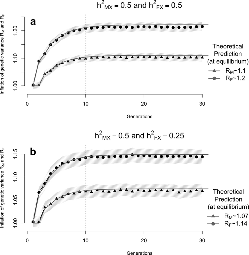
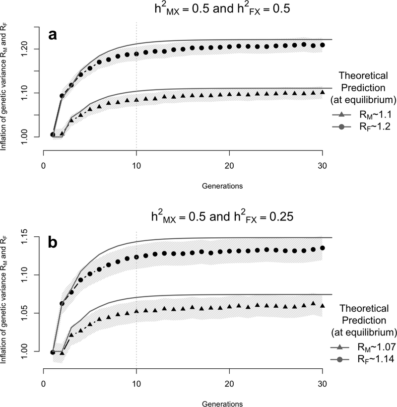
For X-chromosome loci, we also considered two scenarios. These scenarios are characterized by values of the base population heritability in males $\left(h_{MX}^2\right)$ and females $\left(h_{FX}^2\right)$: scenario X1 where $h_{MX}^2=0.5$ and $h_{FX}^2=0.5$ and scenario X2 where $h_{MX}^2=0.5$ and $h_{FX}^2=0.25$. We found in both scenarios a good agreement between observed inflation in genetic variance and predictions assuming normality of breeding values (Figure 3). However, we also observed a slight overestimation from our theoretical predictions, which is explained by the deviation from the normal distribution assumption resulting from the relatively small number of causal loci (M_X = 50 = M/20). More specifically, our averaged estimates over 1,000 simulation replicates are ∼ 10.2% and ∼ 21.5% in males and females respectively in scenario X1 and ∼ 6.9% and ∼ 14.4% in males and females respectively in scenario X2. These estimates are yet consistent with predictions from equations (29) and (28), i.e. (R_M − 1 = 11.07%,R_F − 1 = 22.1%) in scenario X1 and (R_M − 1 = 7.4%,R_F − 1 = 14.9%) in scenario X2. In the latter simulation standard errors of the mean inflation of genetic variance are ∼ 0.8%. These standard errors are larger than reported in the simulations based on autosomal loci since variances were calculated separately for males and females.

Figure 3:

Simulation results showing the inflation of the genetic variance (with 95% confidence interval - light band around each dot) induced by assortative mating (AM) on a quantitative trait controlled by unlinked X-chromosome variants. Data were simulated assuming that the trait driving assortment is controlled by 50 bi-allelic variants with allele frequency p = 0.5. Each simulation replicate generates a population of 2,500 males and 2,500 females undergoing AM for 30 generations with a mate correlation ρ = 0.25. The heritability in males was fixed to $h_{MX}^2=0.5$ and two scenarios were considered corresponding to a heritability in females (1) $h_{FX}^2=0.5$ or (2) $h_{FX}^2=0.25$. The empirical genetic variance is calculated at each iteration as the sampling variance (in males and females separately) of the simulated breeding value from the X-chromosome. The ratio of the empirical genetic variance over the genetic variance in the base population was averaged over 1,000 simulation replicates (each dot corresponds the average over 1,000 simulated populations) and compared with theoretical expectations R_M and R_F from equation (28).

Overall these two simulations (autosome and X-controlled traits) validate the theoretical predictions derived in equations (6), (29) and (28).

Linkage

[2] previously showed, in the absence of selection (which we also assumed here), that linkage has no effect on the inflation of genetic variance under assortative mating. We wished to confirm this result through simulations. We therefore re-did the same simulations described above with the only exception that causal variants were linked within families. We detail how linked loci were simulated in the Appendix section. Overall, we confirmed Bulmer’s result and also show that linkage slows down the speed of convergence towards equilibrium (Figures 5 and 6).

Figure 5:

Simulation results showing the inflation of the genetic variance (with 95% confidence interval - light band around each dot) induced by assortative mating (AM) on a quantitative trait controlled by linked autosomal variants. Data were simulated assuming that the trait driving assortment is controlled by 1,000 linked bi-allelic variants with allele frequency p = 0.5. Details on the simulation of linked loci are given the Appendix section. Two scenarios were considered with either a heritability (1) h² = 0.25 or (2) h² = 0.5. Each simulation replicate generates a population of 2,500 males and 2,500 females undergoing AM for 30 generations with a mate correlation ρ = 0.25. The empirical genetic variance is calculated at each iteration as the sampling variance (over the 5,000 generated individuals) of the simulated breeding value. The ratio of the empirical genetic variance over the genetic variance in the base population was averaged over 1,000 simulation replicates (i.e. 1,000 simulated populations) and compared with theoretical expectation R_A from equation (6). In the first scenario (h² = 0.25, lower dotted curve) R_A ∼ 1.07 and in the second scenario (h² = 0.5, upper plain curve), R_A ∼ 1.15.

Figure 6:

Simulation results showing the inflation of the genetic variance (with 95% confidence interval - light band around each dot) induced by assortative mating (AM) on a quantitative trait controlled by linked X-chromosome variants. Data were simulated assuming that the trait driving assortment is controlled by 50 bi-allelic variants with allele frequency p = 0.5. Details on the simulation of linked loci are given the Appendix section. Each simulation replicate generates a population of 2,500 males and 2,500 females undergoing AM for 30 generations with a mate correlation ρ = 0.25. The heritabily in males was fixed to $h_{MX}^2=0.5$ and two scenarios were considered corresponding to a heritability in females (1) $h_{FX}^2=0.5$ or (2) $h_{FX}^2=0.25$. The empirical genetic variance is calculated at each iteration as the sampling variance (in males and females separately) of the simulated breeding value from the X-chromosome. The ratio of the empirical genetic variance over the genetic variance in the base population was averaged over 1,000 simulation replicates and compared with theoretical expectations R_M and R_F from equation (28).

Validity of equations (18) and (19)

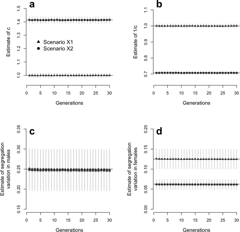
We used the same simulation framework described above to test the validity of equations (18) and (19). Equation (18) predicts that the regression of males breeding values onto their mothers’ yields an unbiased estimate of the scaling parameter c defined above in equation (20) and also that the residual variance of that regression is an estimate of the constant segregation variance in males. Similarly, equation (19) predicts that the regression of females breeding values onto their mothers’ (A_FX) and their fathers’ (A_MX) yields an unbiased estimate of 1/c and that the residual variance of the latter regression is an unbiased estimator of the constant segregation variance in females. We performed these regressions at each generation (t > 1) of our simulation study (scenarios X1 and X2) and monitored the estimates of c, 1/c, var(m_M) and var(m_F ). We show in Figure 7 that all estimators are unbiased, i.e. not significantly different from their expected value under normality assumptions. Therefore, equations (18) and (19) are good approximations of how breeding values in the next generations are determined, even for traits controlled by finite numbers of loci.

Figure 7:

Estimate of dosage compensation (scaling parameter c) and segregation variances in males (var[m_M]) amd females (var[m_F]). These estimates are obtained from the linear regression defined in equations (18) and (19), i.e. from the regression of male and female breeding values onto that of their parents. These regressions are performed at each generation of 1,000 simulated populations undorgoing assortative mating for 30 generations as described in the simulation study (scenarios X1 and X2). Panel a represents estimates of c, expected to be c = 1 and $c=\sqrt{2}\approx 1.414$ in scenarios X1 and X2 respectively. Panel b represents estimates of 1/c. Panel c represents estimates of var[m_M], expected to equal 0.5 in both scenarios X1 and X2. Panel d represents estimates of var[m_F] expected to be var[m_F] = 0.5 and var(m_F) = 0.25 in scenarios X1 and X2 respectively.

Correlation of double first cousins

We ran a simulation to compare predictions of the phenotypic correlation between DFC from equation (16) (from [5]) and equation (17) (from [7]). Since both equations are functions of the product of heritability h² and mates correlation ρ, we fixed in this simulation the heritability to be h² = 1 and varied the mates correlation between ρ = 0, 0.1, 0.2,...,0.9. For each value of ρ, we simulated one population composed of 1,000 males and 1,000 females and simulated AM for 10,000 generations. In this simulation, each sampled mates pairs engendered two offspring. We used such large number of iterations to maximize to chances of observing DFC under simple AM. Once equilibrium reached (after > 10 iterations), we identified all DFC pairs of and calculated their sampling phenotypic correlation.

We found a good consistency between [5] and [7] predictions when ρ < 0.2. For large values of ρ, we found that Fisher’s formula underestimates the correlation between DFC while Gimelfarb’s prediction follows closely the empirical correlation (Figure 4). Note that we have not used in this simulation any of the models proposed by [7] and that DFC in our simulation occurred completely at random (see Appendix).

Discussion

This study reviews some of the most important results of the theory of AM: (i) the increase of genetic variance in the population and (ii) the increase of correlation between relatives, especially for distant relatives. For the former, we proposed beyond existing results, an extension of [2] theory for traits controlled by X-chromosome loci. In particular, we have shown when equilibrium is reached, that the inflation of genetic variance, also referred to as disequilibrium variance, is twice as large in females compared to males. This result is important as it gives insights into reasons why heritability of certain traits may differ between males and females, in particular if these traits are correlated between spouses and controlled by variants on the X-chromosome. Another consequence of our results is that the ratio of genetic variance between males and females is reduced in the equilibrium population as compared to the base population. Regarding the correlation between relatives, we shed the light on inconsistent results regarding DFC and demonstrated through simulations that [5] results are only valid for moderate strength of assortment, and that [7] formula perfectly matches our simulations. As mathemetically demonstrated in [7], the reason of this discrepancy is that [5] ignored that AM modifies the frequency of DFCs in a assortatively mating population relative to a randomly mating population. Our simulations, which do not rely on the assumption of unchanged frequency of DFCs in the population over multiple generations of AM, therefore expose the limitations of [5] formula.

The results presented in this study have some limitations. First, our analyses are restricted to cases where the covariance between relatives is purely genetic and where genetic variation is solely additive. We therefore ignored here the contribution of shared environments and non-additive genetic contributions such as dominance effects. In addition, our extension of [2] to X-chromosome loci was proposed under the normal distribution theory, i.e. assuming a large number of loci contributing to the genetic architecture of the traits. Although, this assumption seems reasonable even for limited number of loci (∼ 10 if allele frequency > 0.1), our theory does not properly cover all examples with finite number of loci. Nevertheless, we show under simplifying assumptions (Appendix section) that our results from equations (6), (29) and (28), hold in a finite locus model.

As large collections of SNP genotyped samples are increasingly accessible, it is now possible to quantify empirically some the consequences of AM. Recent works as those as [17], [15] or [20] exemplify how SNP data can be used to gain insights into the genomic signature of AM, that is the correlation induced by AM between trait-increasing alleles at unlinked loci. This genomic signature was recently quantified in [20] as the correlation between weighted counts of trait-associated alleles (e.g. identified in large genome-wide associations studies) from odd- versus even-numbered chromosomes. Despite progress based on autosomal variants, we still do not have at present sufficiently large numbers of genetic variants on the X-chromosome that are robustly associated with traits driving AM such as height or educational attainment. In the near future however, given the ever constant increase in the size of genome-wide association studies ([10]), such data are likely to become available. We underline also that the theory developed in this study for the X-chromosome has ignored possible effects of sexual selection, which might therefore limit its applicability to real data sets where such selection may be present. Other questions are left unanswered. For example, how large is the gametic phase disequilibrium induced by AM? Or its companion question, how much of the disequibrium variance can we quantify from SNP data? Do empirical observations match with theoretical predictions from [4], and others? In the near future, with the availability of large datasets from genome-wide association studies, these questions can be addressed empirically.

References

- [1].Barton NH, Etheridge AM, and Veber A. The infinitesimal model: Definition, derivation, and implications. Theoretical Population Biology, 118:50–73, December 2017. [DOI] [PubMed] [Google Scholar]
- [2].Bulmer MG. The mathematical theory of quantitative genetics. Clarendon Press, October 1980. [Google Scholar]
- [3].Crow JF and Felsenstein J. The effect of assortative mating on the genetic composition of a population. Social Biology, 29(1–2):22–35, 1982. [PubMed] [Google Scholar]
- [4].Crow JF and Kimura M. An Introduction to Population Genetics Theory. Blackburn Press, 1970. [Google Scholar]
- [5].Fisher RA. The correlation between relatives on the supposition of Mendelian inheritance. Trans. R. Soc. Edinb, pages 399–433, 1918. [Google Scholar]
- [6].Gimelfarb A. Analysis of nontraditional relationships under assortative mating. Journal of Mathematical Biology, 13(2):227–240, December 1981. [Google Scholar]
- [7].Gimelfarb A. A general linear model for the genotypic covariance between relatives under assortative mating. Journal of Mathematical Biology, 13(2):209–226, December 1981. [Google Scholar]
- [8].Jiang Y, Bolnick DI, and Kirkpatrick M. Assortative Mating in Animals. The American Naturalist, 181(6):E125–E138, June 2013. [DOI] [PubMed] [Google Scholar]
- [9].Lynch M and Walsh B. Genetics and Analysis of Quantitative Traits. Sinauer, January 1998. [Google Scholar]
- [10].Manolio TA. A decade of shared genomic associations. Nature, 546(11):360–361, 2017. [DOI] [PubMed] [Google Scholar]
- [11].Nagylaki T. The correlation between relatives with assortative mating. Annals of Human Genetics, 42(1):131–137, July 1978. [DOI] [PubMed] [Google Scholar]
- [12].Nagylaki T. Assortative mating for a quantitative character. Journal of Mathematical Biology, 16(1):57–74, 1982. [DOI] [PubMed] [Google Scholar]
- [13].Pryke Sarah R.. Sex chromosome linkage of mate preference and color signal maintains assortative mating between interbreeding finch morphs. Evolution; International Journal of Organic Evolution, 64(5):1301–1310, May 2010. [DOI] [PubMed] [Google Scholar]
- [14].Risch H. The correlation between relatives under assortative malting for an X-linked and autosomal trait. Annals of Human Genetics, 43(2):151–165, October 1979. [PubMed] [Google Scholar]
- [15].Robinson MR, Kleinman A, Graff M, Vinkhuyzen AAE, Couper D, Miller MB, Peyrot WJ, Abdellaoui A, Zietsch BP, Nolte IM, van Vliet-Ostaptchouk JV, Snieder H, The LifeLines Cohort Study, Genetic Investigation of Anthropometric Traits (GIANT) consortium, Medland SE, Martin NG, Magnusson PKE, Iacono WG, McGue M, North KE, Yang J, and Visscher PM. Genetic evidence of assortative mating in humans. Nature Human Behaviour, 1(1):0016, January 2017. [Google Scholar]
- [16].Saether SA, Saetre G-P, Borge T, Wiley C, Svedin N, Andersson G, Veen T, Haavie J, Servedio MR, Bures S, Kral M, Hjernquist MB, Gustafsson L, Traff J, and Qvarnstrom A. Sex chromosome-linked species recognition and evolution of reproductive isolation in flycatchers. Science (New York, N.Y.), 318(5847):95–97, October 2007. [DOI] [PubMed] [Google Scholar]
- [17].Tenesa A, Rawlik K, Navarro P, and Canela-Xandri O. Genetic determination of height-mediated mate choice. Genome Biology, 16:269, January 2016. [DOI] [PMC free article] [PubMed] [Google Scholar]
- [18].Visscher PM, Brown MA, McCarthy MI, and Yang J. Five years of GWAS discovery. American Journal of Human Genetics, 90(1):7–24, January 2012. [DOI] [PMC free article] [PubMed] [Google Scholar]
- [19].Wright S. Systems of mating. III. Assortative mating based on somatic resemblance. Genetics, 6:144–161., 1921. [DOI] [PMC free article] [PubMed] [Google Scholar]
- [20].Yengo L, Robinson MR, Keller MC, Kemper KE, Yang Y, Trzaskowski M, Gratten J, Turley P, Cesarini D, Benjamin DJ, Wray NR, Yang J, Goddard ME, and Visscher PM. Imprint of Assortative Mating on the Human Genome | bioRxiv, April 2018. [DOI] [PMC free article] [PubMed] [Google Scholar]
Associated Data
This section collects any data citations, data availability statements, or supplementary materials included in this article.