Relatedness of the incidence decay with exponential adjustment (IDEA) model, “Farr's law” and SIR compartmental difference equation models

Abstract

Mathematical models are often regarded as recent innovations in the description and analysis of infectious disease outbreaks and epidemics, but simple mathematical expressions have been in use for projection of epidemic trajectories for more than a century. We recently introduced a single equation model (the incidence decay with exponential adjustment, or IDEA model) that can be used for short-term epidemiological forecasting. In the mid-19th century, Dr. William Farr made the observation that epidemic events rise and fall in a roughly symmetrical pattern that can be approximated by a bell-shaped curve. He noticed that this time-evolution behavior could be captured by a single mathematical formula (“Farr's law”) that could be used for epidemic forecasting. We show here that the IDEA model follows Farr's law, and show that for intuitive assumptions, Farr's Law can be derived from the IDEA model. Moreover, we show that both mathematical approaches, Farr's Law and the IDEA model, resemble solutions of a susceptible-infectious-removed (SIR) compartmental differential-equation model in an asymptotic limit, where the changes of disease transmission respond to control measures, and not only to the depletion of susceptible individuals. This suggests that the concept of the reproduction number $\left({\mathcal{R}}_0\right)$ was implicitly captured in Farr's (pre-microbial era) work, and also suggests that control of epidemics, whether via behavior change or intervention, is as integral to the natural history of epidemics as is the dynamics of disease transmission.

1. Introduction

The control of communicable diseases is an endeavor that has witnessed remarkable successes over the past century; diseases that previously caused large scale mortality have been eradicated (Hinman, 1999; Roeder, Mariner, & Kock, 2013), locally eliminated (Papania et al., 2014), or have been markedly reduced in incidence globally as a result of vaccination, antimicrobial therapy, water and sewage treatment, and advances in food safety (Armstrong, Conn, & Pinner, 1999; Liu et al., 2015; Murray et al., 2014). Nonetheless, the threat of communicable diseases persists; emerging infectious diseases continue to be identified, often in association with changes in human and animal mobility, agricultural practices, environmental degradation, and misuse of antimicrobial therapy (Jones et al., 2008; Keesing et al., 2010; Kuehn, 2010). Recent outbreaks or epidemics associated with MERS coronavirus (Azhar et al., 2014), influenza A (H7N9) (Cowling et al., 2013), and the West African emergence of the Zaire strain of Ebola virus (Baize et al., 2014), have challenged epidemiologists as the natural history, modes of transmission, and/or means of control of these diseases have not been well understood during initial periods of emergence.

When novel infectious diseases emerge or familiar diseases resurge, mathematical models can serve as useful tools for the synthesis of available data, management of uncertainty, and projection of likely epidemic trajectories (Fisman, 2009). While it may be challenging to parameterize detailed mechanistic mathematical models when there is little information on mechanisms of transmission, baseline immunity in a community, or the nature of the infecting pathogen, a number of descriptive approaches exist which may permit fitting, and forecasting, of an epidemic curve. One single equation approach that has been applied to emerging infections is the Richards model, which treats cumulative infections as a logistic growth process (Hsieh & Chen, 2009; Wang, Wu, & Yang, 2012). However, the concept of modeling an epidemic curve as a simple function, without reference to mechanisms of transmission, is in fact much older, and may originate in the work of the English polymath Dr. William Farr (1807–1883), who rose from humble beginnings to become a physician, mathematician, hygienist and protege of Lancet founder Dr. Thomas Wakley (Brownlee, 1915a; Fine, 1979; Greenwood, 1933). Dr. Farr spent almost 40 years at the General Register Office of the United Kingdom, and the esteem in which he was held is apparent in the “letters” he published annually as appendices to the reports of the Registrar General, in which he supplemented the dry statistical reports with thoughtful and creative musings on topics as wide-ranging as the relationships between occupation and disease, suicide and mortality in the mentally ill, population density and mortality, and as above the “laws” governing epidemics (Farr, 1840).

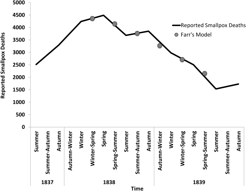
William Farr's analysis is a classic in the epidemiology literature. Farr examined the course of mortality attributable to smallpox between mid 1837 (when death registration was introduced into England and Wales) and 1839, and noted that the numbers peaked in the spring quarter of 1838 and then declined until summer 1839 (Fig. 1) (Farr, 1840). He noted that the pattern of decline was very close to what would be predicted if the ratios of cases in successive quarters declined at a constant rate. He provided numbers demonstrating this in his annual report to the Registrar General in 1840 (Fig. 1), but did not develop the idea at length. Looking back on this, we may note that this approach is analogous to assuming that the number of transmissions per case (or the “reproduction number” in modern terminology), were to decline at a constant rate during the course of an epidemic. The key difference is that Farr worked before the germ theory, and analysed data in terms of successive calendar time periods rather than successive generations of cases. There is a further irony to the story, in that he never returned to this idea until 1866, at which time there was a major epidemic of rinderpest, which some feared would destroy the British cattle population (Brownlee, 1915a). Farr applied a similar analysis, but this time based upon assuming that the third ratio of cases per month was a constant (in effect assuming that the reproduction number declined at a constantly accelerating pace). He used this approach to predict that the epidemic would decline rapidly over the subsequent six months, and published this, including predicted monthly incidence numbers, in the Daily News of London in February 1866. His predictions were close to what subsequently happened (Brownlee, 1915a).

Fig. 1.

A recreation of William Farr's possible approach modeling the decline in smallpox mortality in England, 1837–1839 (Farr, 1840). Black line, smallpox mortality by season; gray dots represent Farr's “model projections” derived by assuming a constant additive increase (approximately 5% per season) in the decline in smallpox deaths. Farr “smoothed” reported seasonal deaths by averaging adjacent seasons; hence model projections are plotted at the midpoint (e.g., “winter-spring”, “spring-summer”) at each interval.

It fell to other contemporaries (Evans, 1876) and later epidemiologists (most notably Dr. John Brownlee) to formalize “Farr's law” (Brownlee, 1915c; Fine, 1979; Serfling, 1952). (It should be noted that the term “Farr's law” is ambiguous. Farr himself referred to a “law” in his letter on rinderpest (Brownlee, 1915a), but the term has also been used by others to describe Farr's observations on the relation between population density and death (Brownlee, 1915b), and to his description of the relationship between cholera mortality and altitude (Lilienfeld, 2007). In his elaboration of the “law”, Brownlee referred to it as “Farr's theory of epidemics” (Brownlee, 1915a)).

We recently proposed a descriptive approach to the initial estimation of the basic reproduction number $\left({\mathcal{R}}_0\right)$ of an emerging or re-emerging pathogen, which also provides information on the rate at which the process is being controlled, as well as reasonable short-term projections of incidence. This two-parameter model, which we have referred to as the “Incidence Decay with Exponential Adjustment” (IDEA) model, offers advantages of simplicity, explicit linkage to theory of epidemic growth, and also acknowledges the fact that epidemics and outbreaks do not peak and end simply due to depletion of susceptibles, but because of a complex constellation of public health actions and behavioral changes that may modify the course of an epidemic and reduce the effective reproduction number ${\mathcal{R}}_e\left(t\right)$ during an outbreak (Fisman et al., 2013). In our previously published description of this model, we validated model projections by showing that they were identical to those derived from a discrete-time susceptible-infectious-removed (SIR) compartmental model, provided the SIR model had a low basic reproduction number $\left({\mathcal{R}}_0\right)$ and exponential improvement in control over the course of the epidemic (Fisman et al., 2013).

One of us (PF) had previously written about Farr's law and its importance in the development of epidemic theory (Fine, 1979), and noted the conceptual similarity between IDEA and Farr's law. Upon exploration of these two approaches we realized that they, notwithstanding having been formulated some 160 years apart, and being based on very different theoretical constructs, are fully consistent with one another. Here we demonstrate the equivalence of these methods for epidemic modeling and forecasting, explore the potential advantages of using these methods to complement other approaches, and identify the circumstances under which these methods closely approximate the commonly-used SIR modeling approach. We explore numerical examples derived from recent emerging infectious diseases, including 2014–2015 West African Ebola virus outbreak. We show that these methods work fairly well in a number of cases, and discuss what this fact implies about difficult-to-measure components of transmission and control parameters.

2. Methods

2.1. Farr's law

The empirical relationship between observed cases of infected individuals, in sequential time intervals, during an epidemic outbreak according to Farr's law is given by

$$\frac{\left(\frac{I\left(t+3\right)}{I\left(t+2\right)}\right)}{\left(\frac{I\left(t+1\right)}{I\left(t\right)}\right)}=K$$ (1)

where $I\left(t\right)$ represents the number of observed newly infected individuals at time t, and K is a constant. For values of $K<1$, the rate of change in the observed cases (acceleration) decreases as time evolves, and the family of curves $I\left(t\right)$ that satisfy equation (1) correspond to familiar bell-shaped epidemic curves.

The law was investigated and elaborated upon by the epidemiologist John Brownlee who noted that $I\left(t\right)$ under this law would correspond to the function (Fine, 1979)

$$\text{exp}\left(-A{t}^2+Bt+C\right)$$ (2)

where A, B, and C are constants. Of note, Brownlee's formulation identifies a process by which cases increase as a first order process, but decrease as a second order process, as is the case with the IDEA model.

2.2. IDEA model

In the basic form of the IDEA model, the time evolution of infected cases, $I\left(t\right)$, satisfies equation (3),

$$I\left(t\right)={\left(\frac{{\mathcal{R}}_0}{{\left(1+d\right)}^t}\right)}^t$$ (3)

where t is an integer “generation” of an outbreak (thus $t=\left\{\mathrm{1,2,3},\dots \right\}\in \mathrm{\mathbb{N}}$). In other words, in the IDEA model, the unit of time is the generation interval (the time interval between the time when an individual is infected by an infector and the time when this infector was infected). In Farr's model, t is the time at which subsequent observation are made.

The parameter ${\mathcal{R}}_0$ is the basic reproduction number as usually defined; that is, the number of secondary cases created by a primary case in a totally susceptible population and in the absence of intervention. The parameter $d>0$ which we have referred to as a “control parameter” defines the rate at which transmission declines over the course of an epidemic. The empirical underpinnings of d are not yet well defined, but based on current understanding of disease dynamics could represent public health interventions, population adaptation or behavior change, improved availability of personal protective items or effect of drugs to treat infection, or reductions in population susceptibility as a result of immunity or vaccination. As noted above, by fitting the model to data we have previously obtained reasonable estimates of ${\mathcal{R}}_0$ early in the course of epidemics, and have also been able to produce plausible near-term projections of future case counts.

2.3. Difference equation susceptible-infectious-removed model

In an earlier publication we commented on the almost identical projections generated by IDEA and a compartmental difference equation (Susceptible-Infectious-Removed, or SIR) (Fisman et al., 2013), in the asymptotic limit when ${\mathcal{R}}_0$ is small and when there is exponential reduction in risk over time. Below we generalize this model equivalence, to any situation where the depletion of susceptibles due to infection is small relative to the total population size (and not only when ${\mathcal{R}}_0$ is small). We used a “damped” version of the standard SIR model whose formulation in generation interval time scale is given by:

$$S_{t+1}=S_t-{\mathcal{R}}_e\left(t\right)I_t$$ (4)

$$I_{t+1}={\mathcal{R}}_e\left(t\right)I_t$$ (5)

with $S_t$ the number of susceptible individuals at time t and ${\mathcal{R}}_e\left(t\right)$ the effective reproduction number at time t defined by:

$${\mathcal{R}}_e\left(t\right)={\mathcal{R}}_0\frac{S_t}{N}{\rho }^t$$ (6)

The “damping” parameter ρ represents the relative risk of infection in each generation of the epidemic, compared to the risk seen in the last generation (i.e., if there were no improvement in control in a given generation compared to the last, most recent generation). If an outbreak is small relative to the size of the total population (as would be true if ${\mathcal{R}}_0$ were modest and control achieved relatively quickly) $S\left(t\right)/N$ will be approximately 1 throughout the outbreak and the expression can be rewritten as:

$$I\left(t\right)=I\left(0\right)\prod _{s<t}\left({\rho }^s{\mathcal{R}}_0\right)$$ (7)

meaning that all reduction in ${\mathcal{R}}_e\left(t\right)$ is due to control rather than depletion of susceptibles. ${\mathcal{R}}_0$ is a constant, and the sum of exponents of ρ is simply $t\left(t+1\right)/2$. We can assume (as we do with IDEA) that the outbreak began with the introduction of a single case such that $I\left(0\right)$  = 1. Now:

$$I\left(t\right)={\rho }^{t\left(t+1\right)/2}{\mathcal{R}}_0^t$$ (8)

Numerical simulations were implemented in the R software (Theroject for Statist, 2015) and code is available in electronic supplement files (Supporting Information: Supplement 1).

2.4. Numerical examples using recent outbreak data

We have previously used IDEA to explore the nature of epidemic growth during the recent West African Ebola epidemic (Fisman & Tuite, 2014; Fisman, Khoo, & Tuite, 2014) and the more recent Chikungunya virus invasion in the Western hemisphere (Nasserie, Fisman, & Tuite, 2015). As publicly available data have taken the form of cumulative incidence curves (with absent dates of onset) we fit IDEA to cumulative curves, but it is possible to estimate incidence by taking the interval to interval difference cumulative incidence over time.

Here we fit IDEA to the incidence time series and calculated Farr's K for sequential generation tetrads, and converted K values to the d parameter in IDEA using the relation $K=\frac{1}{{\left(1+d\right)}^4}$ described below. Model fits were performed in a Microsoft Excel spreadsheet using the Solver add-in. Data sources used for these analyses are available at http://figshare.com/authors/Tahmina_Nasserie/686527 (Chikungunya) and https://github.com/cmrivers/ebola (Ebola). The Original Microsoft Excel files have been included as Supplemental Information.

3. Results

3.1. Equivalence of IDEA and Farr's law

We need to show both, (A) that the IDEA model satisfies Farr's Law, and (B) that Farr's Law can be derived from the IDEA model. This equivalence requires the intuitive assumption that t in Farr's Law (the subsequent times at which observations are made) are integer values and coincide with the serial (or generation) time interval in the IDEA model.

(A) An incidence curve described by IDEA naturally satisfies Farr's law. Indeed, substituting (3) into (1) gives (see Appendix 1):

$$K=\frac{1}{{\left(1+d\right)}^4}$$ (9)

It is interesting to note that the value of ${\mathcal{R}}_0$ in the IDEA model is irrelevant in the proof presented in Appendix 1.

(B) On the other hand, by expressing the IDEA model as

$$I\left(t\right)={\left(\frac{{\mathcal{R}}_0}{{\left(1+d\right)}^t}\right)}^t=\text{exp}\left(t\log \frac{{\mathcal{R}}_0}{{\left(1+d\right)}^t}\right)=\text{exp}\left(-t^2\log \left(1+d\right)+t\log {\mathcal{R}}_0\right)$$ (10)

we see that we recover John Brownlee's Gaussian curve (2) with $A=\text{log}\left(1+d\right)$, $B=\text{log}{\mathcal{R}}_0$ and $C=0$ that recapitulates Farr's Law as stated in Equation (1).

3.2. Relation of SIR model to Farr's K and IDEA

When the depletion of susceptibles is negligible compared to the total population size (that is, a small outbreak), we can actually express IDEA's basic reproduction number ${\mathcal{R}}_{0,IDEA}$ and its control factor d as a function of the basic reproduction number ${\mathcal{R}}_{0,SIR}$ and the control factor ρ of the damped SIR model described in (4–6). The relationship between the parameters of these two models is:

$${\mathcal{R}}_{0,IDEA}\simeq \frac{{\mathcal{R}}_{0,SIR}}{\sqrt{\rho }}$$ (11)

$$d\simeq \frac{1}{\sqrt{\rho }}-1$$ (12)

Note that both equations (11), (12) are only sufficient conditions for the respective parameters of both models to produce the same incidence when the size of the epidemic is negligible compared to the total size of the population (see Appendix 2).

Substituting (12) in equation (9) we can link Farr's law with the damped SIR model:

$$K\simeq {\rho }^2$$ (13)

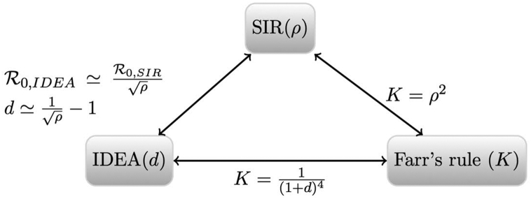
The relationship between Farr's law, the IDEA model, and the damped SIR model is illustrated graphically in (Fig. 2).

Fig. 2.

Relationship between the three models. Parameter ρ represent the relative risk of infection in each generation for the SIR model. The control parameter d is associated with the IDEA model and K is Farr's ratio.

3.3. Numerical simulations

In this section, we aim to test numerically the validity of approximations (11), (12). In particular, given a damped SIR model, we explore the parameter space ${\mathcal{R}}_{0,SIR}$ and ρ for which these approximations hold. Note that the link between IDEA and Farr's law given by equation (9) is not an approximation, but a genuine equality (subject to the time step used in Farr's law being equivalent to one generation), so there is no need to test it numerically. To measure the performance of the approximation, we consider the distance between the simulated incidence time series. Let N be the number of generations simulated and $I_{SIR}\left(k\right)$ (resp. $I_{IDEA}\left(k\right)$) the incidence from the SIR (resp IDEA) model at the $k^{th}$ generation, we define their distance by

$$\delta =\sqrt{\sum _{k=1}^N{\left(I_{SIR}\left(k\right)-I_{IDEA}\left(k\right)\right)}^2}$$ (14)

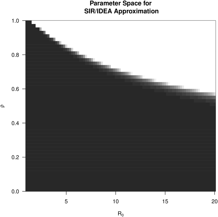
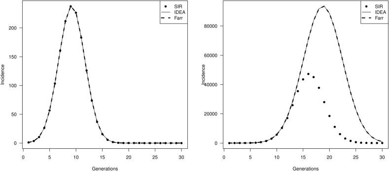
Fig. 3 shows the values of the distance δ for different values of ${\mathcal{R}}_{0,SIR}$ and ρ. We see that for a combination of ${\mathcal{R}}_{0,SIR}$ and ρ such that the depletion of susceptible is not too large, the approximation is very good. But when the values of ${\mathcal{R}}_{0,SIR}$ and ρ generate a depletion of susceptible individuals that is no longer negligible (white area in Fig. 3), then the incidence curve from the IDEA model diverges from that generated by the damped SIR model. This is demonstrated in Fig. 4.

Fig. 3.

A heat map plotting values for ${\mathcal{R}}_{0,SIR}$ and ρ where the damped SIR model can be approximated by a IDEA model using equations (11), (12). Darker areas indicate a good match (measured as the sum of squared differences) between the simulated incidence time series; lighter areas represent combinations of values for which incidence time series for SIR and IDEA diverge.

Fig. 4.

Evaluation of IDEA model fit to simulated data derived from the damped SIR model. Left panel illustrates a scenario where approximation is very good, (${\mathcal{R}}_{0,SIR}=3.5$, $\rho =0.85$), corresponding to a combination of values found in the dark area in Fig. 3. The right sided panel uses a combination of values (high ${\mathcal{R}}_{0,SIR}$ and/or low ρ) where susceptible depletion cannot be ignored (i.e., corresponding to the white area in Fig. 3 3). It can be seen that IDEA and the damped SIR models diverge when susceptibles are rapidly depleted.

3.4. Application: ebola and Chikungunya

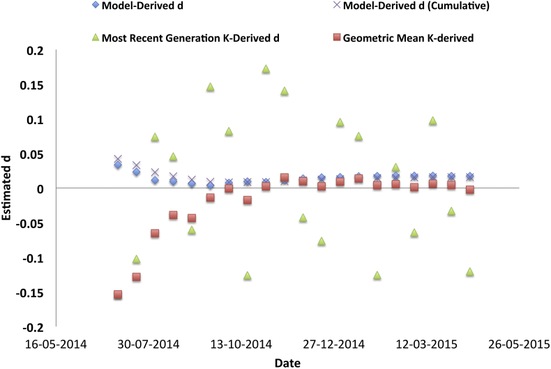
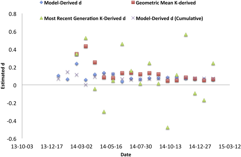
Considering real epidemic data from Ebola and Chinkungunya, it can be seen that the interval to interval variability in K was substantial, likely reflecting variability in reporting (Fig. 5, Fig. 6). Simple arithmetic means of K over time were also unstable due to skewing by values substantially greater than 1. However, when we estimated the geometric mean of K over time we found that the resultant d estimate approximated that derived through fitting IDEA.

Fig. 5.

The graph plots estimates of IDEA d parameter against time during the recent West African Ebola outbreak. Approximate date of the last generation incorporated into estimates is plotted on the X-axis; estimated d is plotted on the Y-axis. d estimates were either derived via IDEA model fitting to “incident” cases (blue diamonds) or cumulative incidence (crosses), or derived by estimating Farr's K and transforming resultant estimates using the relation described by equation (9). When K is estimated using 4-generation series (green diamonds), resultant d estimates are volatile and bear little resemblance to d estimates derived through fitting IDEA. However, estimates of K derived as geometric means of all available K values (red squares) provide a more reasonable approximation of d.

Fig. 6.

As with Fig. 5, this figure shows estimates of d, derived directly by model fitting or by transforming estimates of Farr's K, for the emerging Western Hemisphere Chikungunya epidemic in 2014–2015. As in Fig. 5, d estimates were either derived via IDEA model fitting to “incident” cases (blue diamonds) or cumulative incidence (crosses), or derived by estimating Farr's K and transforming resultant estimates. As in Fig. 5, volatile estimates of K were derived using 4-generation series (green diamonds), but estimates of K derived as geometric means of all available K values (red squares) provided a reasonable approximation of d.

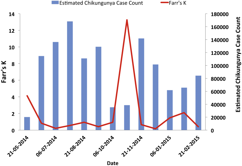
Furthermore, we noted that in the Chikungunya time series there was a large perturbation in best-fit values of d occurring in October 2014, corresponding with an apparent multi-wave epidemic. We have previously noted that this abrupt change in the generation-to-generation best fit value of d corresponds with the occurrence of multiwave epidemics when IDEA is fit to simulated data (Fisman et al., 2013); using Farr's approach, the onset of a possible new Chikungunya wave seems to correspond with an abrupt increase in K to a value far greater than one (Fig. 7). The utility of large values of K as a signal of an incipient epidemic wave warrants further investigation.

Fig. 7.

A possible application for raw estimates of Farr's K emerged in analysis of data from the 2014–2015 Western Hemisphere Chikungunya outbreak; here it appears that a multi-wave epidemic is signaled by a sudden surge in K to a value $>1$ (red line), indicating that there is renewed exponential growth in cases (blue bars), rather than exponential decline. X-axis, date of most recent generation; left Y-axis, Farr's K; right Y-axis, estimated per-generation Chikungunya case count and transforming resultant estimates. As in Fig. 1, volatile estimates of K were derived using 4-generation series (green diamonds), but estimates of K derived as geometric means of all available K values (red squares) provided a reasonable approximation of d.

4. Discussion

Although the real-time application of mathematical modeling to understanding and control of outbreaks is often perceived as representing a recent development in infectious disease epidemiology (Heesterbeek et al., 2015), disease modeling has deeper historical roots, including work by Bernoulli on smallpox in the 18th century (Greenwood, 1941); work by Ross on malaria transmission (Smith et al., 2012), and as mentioned above, Farr's work on the growth and cessation of epidemics (Brownlee, 1915a, 1915c; Fine, 1979). We had published a simple, phenomenological approach to the description and projection of outbreaks and epidemics (Fisman et al., 2013) which we had initially regarded as a novel formulation rooted in the concept of the basic reproduction number ${\mathcal{R}}_0$.

In that work, we demonstrated concordance with projections derived using a 3-compartment difference equation model (damped SIR model). We have subsequently realized, and demonstrate above, that our approach simply represented a restatement of Farr's work, albeit in a manner that is tied to the concept of ${\mathcal{R}}_0$. According to Brownlee, Farr promised to describe the derivation of his model in greater detail in future reports, but never did so (Brownlee, 1915a), and much of the mathematical elaboration of Farr's work was in fact done by Brownlee after Farr's death (Brownlee, 1915c). Nonetheless, Brownlee notes that to Farr, the predictive accuracy of his approach reflected three characteristics of epidemics, according to Farr's (pre-microbial) understanding: (i) diminution in the number of susceptibles over time due to recovery from infection (“immunity”, though to use this term in application to Farr is an anachronism); (ii) diminished population density due to death from infection; and (iii) diminishing pathogenicity of the disease with each passing generation of infection as a result of (to quote Farr) “[loss of] part of the force of infection in every body through which they pass…the matter…diminishes in strength at every transmission by innoculation” (Brownlee, 1915a). The first two characteristics are not incompatible with the current understanding of epidemic dynamics, whereas the third is not (though it does anticipate more modern ideas around evolution of virulence and disease ecology (Ewald, 2004; Lipsitch & Moxon, 1997)).

However, as this model is phenomenological, rather than mechanistic in nature, the putative epidemiological mechanisms underlying model performance are not of immediate importance. Indeed, while the simplicity of this approach may be regarded as a limitation, the simplicity of the form, and its implicit incorporation of biological, social, medical, and behavioral drivers of control into a single parameter estimated via fitting, may be a strength, especially given that such control factors as behavior change due to fear may be difficult or impossible to measure in real time.

When we applied IDEA to current day outbreaks and epidemics, we have remained agnostic about the factors that cause second order deceleration of epidemic growth. Referring to first principles, the components of a reproduction number are duration of infectiousness, contact rate, and probability of transmission conditional on contact, as well as susceptibility in a population (Vynnycky & White, 2010). We presume that public health interventions, population behavior change (as a result of education or rumours, prudence or fear), and the occurrence of silent infections with immunity could all contribute to deceleration of epidemic spread, even when the effective reproduction number is expected to be greater than 1 due to widespread susceptibility in the population. Furthermore, we note that Farr's original “time step” appears to have been arbitrary (reflecting the form of data available to him: weekly for rinderpest, quarterly for smallpox), whereas we have used generations as time steps in our more recent applications of Farr's “law”, and in IDEA and SIR models. This potential discrepancy between Farr's initial efforts and our more recent efforts can be addressed by a simple rescaling of the time parameter, and is thus immaterial to our conclusions.

5. Summary

In demonstrating that the IDEA model and Farr's model are mathematically equivalent (and can be virtually identical to an SIR model with abundant susceptibility in the population) we demonstrate that recognizing the underlying mechanism of epidemic control may be unimportant for generating reasonable forecasts of epidemics with control, or recognizing when their fundamental dynamics have changed. Our contribution in the current work is to show that Farr's law, while derived in the pre-microbial era, can be reformulated in terms of the concept of the basic reproduction number, combined with exponential increase in control via an unspecified mechanism. We observe, unexpectedly, that Farr's K can be expressed as a function of the IDEA d parameter alone, independent of ${\mathcal{R}}_0$, implying that epidemic trajectory is (and has historically been) more a function of control efforts and changing behavior than of the fundamental characteristics of a given infectious disease. Whether or not the ratio K can have stand-alone value as a tool to identify unexpected shifts in epidemic trajectory (e.g., the two wave epidemic of Chikungunya referred to in Fig. 7 above) will be the subject of future work.

Handling Editor: Jianhong Wu

Appendix 1. Details on IDEA and Farr's law relationship

Assume that the parameters ${\mathcal{R}}_0$ and $d\ge 0$, in the IDEA model, describe accurately the observed number of infected cases as a function of (serial) time, in an ideal outbreak. Then we can substitute $I\left(t\right)$ from equation (3) into equation (1) to see if the sequential number of infected individuals, as predicted by the IDEA model, satisfy Farr's law.

For clarity, choose $t=1$, thus equation (1) becomes

$$\begin{array}{c}\frac{\left(\frac{I\left(4\right)}{I\left(3\right)}\right)}{\left(\frac{I\left(2\right)}{I\left(1\right)}\right)}=\frac{\frac{{\left(\frac{{\mathcal{R}}_0}{{\left(1+d\right)}^4}\right)}^4}{{\left(\frac{{\mathcal{R}}_0}{{\left(1+d\right)}^3}\right)}^3}}{\frac{{\left(\frac{{\mathcal{R}}_0}{{\left(1+d\right)}^2}\right)}^2}{\left(\frac{{\mathcal{R}}_0}{\left(1+d\right)}\right)}}=\frac{\left(\frac{{\mathcal{R}}_0^4}{{\mathcal{R}}_0^3}\right)\left(\frac{{\left({\left(1+d\right)}^3\right)}^3}{{\left({\left(1+d\right)}^4\right)}^4}f\right)}{\left(\frac{{\mathcal{R}}_0^2}{{\mathcal{R}}_0}\right)\left(\frac{\left(1+d\right)}{{\left({\left(1+d\right)}^2\right)}^2}\right)}\\ =\frac{{\mathcal{R}}_0\left(\frac{{\left(1+d\right)}^9}{{\left(1+d\right)}^{16}}\right)}{{\mathcal{R}}_0\left(\frac{\left(1+d\right)}{{\left(1+d\right)}^4}\right)}=\frac{{\left(1+d\right)}^{-7}}{{\left(1+d\right)}^{-3}}=\frac{1}{{\left(1+d\right)}^4}\end{array}$$

By identifying the constant $K=1/{\left(1+d\right)}^4$, the IDEA model satisfies Farr's law for $t=1$. In general, for any sequential (integer) time intervals $t,t+1,t+2,t+3$ one can generalize the above result as follows:

$$\begin{array}{c}\frac{\left(\frac{I\left(t+3\right)}{I\left(t+2\right)}\right)}{\left(\frac{I\left(t+1\right)}{I\left(t\right)}\right)}=\frac{\frac{{\left(\frac{{\mathcal{R}}_0}{{\left(1+d\right)}^{t+3}}\right)}^{t+3}}{{\left(\frac{{\mathcal{R}}_0}{{\left(1+d\right)}^{t+2}}\right)}^{t+2}}}{\frac{{\left(\frac{{\mathcal{R}}_0}{{\left(1+d\right)}^{t+1}}\right)}^{t+1}}{{\left(\frac{{\mathcal{R}}_0}{{\left(1+d\right)}^t}\right)}^t}}=\frac{\left(\frac{{\mathcal{R}}_0^{t+3}}{{\mathcal{R}}_0^{t+2}}\right)\left(\frac{{\left({\left(1+d\right)}^{t+2}\right)}^{t+2}}{{\left({\left(1+d\right)}^{t+3}\right)}^{t+3}}\right)}{\left(\frac{{\mathcal{R}}_0^{t+1}}{{\mathcal{R}}_0^t}\right)\left(\frac{{\left({\left(1+d\right)}^t\right)}^t}{{\left({\left(1+d\right)}^{t+1}\right)}^{t+1}}\right)}\\ =\frac{{\mathcal{R}}_0\left(\frac{{\left(1+d\right)}^{{\left(t+2\right)}^2}}{{\left(1+d\right)}^{{\left(t+3\right)}^2}}\right)}{{\mathcal{R}}_0\left(\frac{{\left(1+d\right)}^{t^2}}{{\left(1+d\right)}^{{\left(t+1\right)}^2}}\right)}=\frac{{\left(1+d\right)}^{{\left(t+2\right)}^2-{\left(t+3\right)}^2}}{{\left(1+d\right)}^{t^2-{\left(t+1\right)}^2}}\\ =\frac{{\left(1+d\right)}^{-2t-5}}{{\left(1+d\right)}^{-2t-1}}=\frac{1}{{\left(1+d\right)}^4}\end{array}$$

Appendix 2. Details on IDEA and SIR relationship

Incidence or the SIR model (Equation (4)) can be written as

$$\begin{array}{c}{I}_t^{SIR}=RE\left(t\right)I_{t-1}\\ =I_0\stackrel{t-1}{\prod _{h=0}}RE\left(s\right)\\ =I_0\stackrel{t-1}{\prod _{h=0}}{R}_{0,SIR}{S}_h/N{\rho }^h\\ =R_{0,SIR}^t{\rho }^{t\left(t-1\right)/2}\stackrel{t-1}{\prod _{h=0}}{S}_h/N\end{array}$$

If the epidemic size is small compared to the size of the whole population, then it can be assumed that

$$\prod _{h=0}^{t-1}\left(\frac{S_h}{N}\right)\simeq 1$$

In that case,

$$I_t^{SIR}\simeq {\mathcal{R}}_{0,SIR}^t{\rho }^{t\left(t-1\right)/2}=\frac{{\left({\mathcal{R}}_{0,SIR}/\sqrt{\rho }\right)}^t}{{\left(1/\sqrt{\rho }\right)}^{t^2}}$$ (15)

Incidence in the IDEA framework is simply

$$I_t^{IDEA}={\left(\frac{{\mathcal{R}}_{0,IDEA}}{{\left(1+d\right)}^t}\right)}^t=\frac{{\mathcal{R}}_{0,IDEA}^t}{{\left(1+d\right)}^{t^2}}$$ (16)

Finally, both models have the same incidence at time t if $I_t^{SIR}=I_t^{IDEA}$. A sufficient condition for that equality to hold is when both numerator and denominator of equations (15), (16) are equal, that is

$$\begin{array}{l}{\mathcal{R}}_{0,IDEA}\simeq \frac{{\mathcal{R}}_{0,SIR}}{\sqrt{\rho }}\\ d\simeq \frac{1}{\sqrt{\rho }}-1\end{array}$$

Appendix A. Supplementary data

The following are the supplementary data related to this article:

References

- Armstrong G.L., Conn L.A., Pinner R.W. Trends in infectious disease mortality in the United States during the 20th century. Journal of the American Medical Association. 1999;281:61–66. doi: 10.1001/jama.281.1.61. [DOI] [PubMed] [Google Scholar]
- Azhar E.I. Evidence for camel-to-human transmission of MERS coronavirus. New England Journal of Medicine. 2014;370:2499–2505. doi: 10.1056/NEJMoa1401505. [DOI] [PubMed] [Google Scholar]
- Baize S., Pannetier D., Oestereich L. Emergence of Zaire ebola virus disease in Guinea. New England Journal of Medicine. 2014;371:1418–1425. doi: 10.1056/NEJMoa1404505. [DOI] [PubMed] [Google Scholar]
- Brownlee J. Historical note on Farr's theory of the epidemic. British Medical Journal. 1915;2:250–252. doi: 10.1136/bmj.2.2850.250. [DOI] [PMC free article] [PubMed] [Google Scholar]
- Brownlee J. Studies in the meaning and relationships of birth and death rates II: Density of population and death rate (Farr's law) The Journal of Hygiene. 1915;15:11–16. doi: 10.1017/s0022172400006082. [DOI] [PMC free article] [PubMed] [Google Scholar]
- Brownlee J. On the curve of the epidemic. British Medical Journal. 1915;2:799–800. doi: 10.1136/bmj.1.2836.799. [DOI] [PMC free article] [PubMed] [Google Scholar]
- Cowling B.J. Comparative epidemiology of human infections with avian influenza A H7N9 and H5N1 viruses in China: A population-based study of laboratory-confirmed cases. Lancet—. 2013;382:129–137. doi: 10.1016/S0140-6736(13)61171-X. [DOI] [PMC free article] [PubMed] [Google Scholar]
- Evans G.H. Vol. 3. Hardwicke and Bogue; London: 1876. pp. 551–555. (Some arithmetical considerations on the progress of epidemics). Transactions of the Epidemiological Society of London, Sessions 1866-1876. [PMC free article] [PubMed] [Google Scholar]
- Ewald P. Evolution of virulence. Infectious Disease Clinics of North America. 2004;18:1–15. doi: 10.1016/S0891-5520(03)00099-0. [DOI] [PMC free article] [PubMed] [Google Scholar]
- Farr W. UK. General Register Office; London: 1840. Appendix to the second annual report of the registrar-general.http://histpop.org/ohpr/servlet/PageBrowser2?ResourceType=Registrar Online Historical Population Reports. Available via the Internet at. [Google Scholar]
- Fine P.E.M. John Brownlee and the measurement of infectiousness: An historical study in epidemic theory. Journal of the Royal Statistical Society. Series A. 1979;142:347–362. [Google Scholar]
- Fisman D. Modelling an influenza pandemic: A guide for the perplexed. Canadian Medical Association Journal. 2009;181:171–173. doi: 10.1503/cmaj.090885. [DOI] [PMC free article] [PubMed] [Google Scholar]
- Fisman D.N. An IDEA for short term outbreak projection: Nearcasting using the basic reproduction number. Public Library of Science One. 2013;8:e83622. doi: 10.1371/journal.pone.0083622. [DOI] [PMC free article] [PubMed] [Google Scholar]
- Fisman D.N., Khoo E., Tuite A.R. 8 September 2014. Early epidemic dynamics of the West african 2014 ebola outbreak: Estimates derived with a simple two-parameter model. Public library of science currents. Published online. [DOI] [PMC free article] [PubMed] [Google Scholar]
- Fisman D.N., Tuite A. 21 November 2014. Projected impact of vaccination timing and dose availability on the course of the 2014 West African Ebola epidemic. Public Library of Science Currents. Published online. [DOI] [PMC free article] [PubMed] [Google Scholar]
- Greenwood M. William Farr. Lancet. 1933;5724:1047–1052. [Google Scholar]
- Greenwood M. Medical statistics from graunt to Farr. Biometrika. 1941;32:101–127. [Google Scholar]
- Heesterbeek H. Modeling infectious disease dynamics in the complex landscape of global health. Science. 2015;347 doi: 10.1126/science.aaa4339. aaa4339. [DOI] [PMC free article] [PubMed] [Google Scholar]
- Hinman A. Eradication of vaccine-preventable diseases. Annual Review of Public Health. 1999;20:211–229. doi: 10.1146/annurev.publhealth.20.1.211. [DOI] [PubMed] [Google Scholar]
- Hsieh Y.H., Chen C.W. Turning points, reproduction number, and impact of climatological events for multi-wave dengue outbreaks. Tropical Medicine & International Health. 2009;14:628–638. doi: 10.1111/j.1365-3156.2009.02277.x. [DOI] [PubMed] [Google Scholar]
- Jones K.E. Global trends in emerging infectious diseases. Nature. 2008;451:990–993. doi: 10.1038/nature06536. [DOI] [PMC free article] [PubMed] [Google Scholar]
- Keesing F. Impacts of biodiversity on the emergence and transmission of infectious diseases. Nature. 2010;468:647–652. doi: 10.1038/nature09575. [DOI] [PMC free article] [PubMed] [Google Scholar]
- Kuehn B.M. Human, animal, ecosystem health all key to curbing emerging infectious diseases. Journal of the American Medical Association. 2010;303:117–118. doi: 10.1001/jama.2009.1896. 124. [DOI] [PubMed] [Google Scholar]
- Lilienfeld D.E. Celebration: William Farr (1807–1883) - an appreciation on the 200th anniversary of his birth. International Journal of Epidemiology. 2007;36:985–987. [Google Scholar]
- Lipsitch M.L., Moxon E.R. Virulence and transmissibility of pathogens: What is the relationship? Trends in Microbiology. 1997;5:31–37. doi: 10.1016/S0966-842X(97)81772-6. [DOI] [PubMed] [Google Scholar]
- Liu L. Global, regional, and national causes of child mortality in 2000-13, with projections to inform post-2015 priorities: An updated systematic analysis. Lancet. 2015;385:430–440. doi: 10.1016/S0140-6736(14)61698-6. [DOI] [PubMed] [Google Scholar]
- Murray C.J. Global, regional, and national incidence and mortality for HIV, tuberculosis, and malaria during 1990-2013: A systematic analysis for the global burden of disease study 2013. Lancet. 2014;384:1005–1070. doi: 10.1016/S0140-6736(14)60844-8. [DOI] [PMC free article] [PubMed] [Google Scholar]
- Nasserie T., Fisman D.N., Tuite A.R. Using the incidence decay with exponential adjustment model to understand Chikungunya epidemic growth in the Americas [conference presentation]. Canadian society for epidemiology and biostatistics 2015 conference. Mississauga, Ontario, Canada. June 1-4. 2015. [Google Scholar]
- Papania M.J. Elimination of endemic measles, rubella, and congenital rubella syndrome from the western hemisphere: The US experience. Journal of the American Medical Association Pediatrics. 2014;168:148–155. doi: 10.1001/jamapediatrics.2013.4342. [DOI] [PubMed] [Google Scholar]
- The R Project for Statistical Computing. Available via the Internet at https://www.r-project.org/. Last accessed November 25, 2015.
- Roeder P., Mariner J., Kock R. Rinderpest: The veterinary perspective on eradication. Philosophical Transactions of the Royal Society of London. Series B, Biological Sciences. 2013;368:20120139. doi: 10.1098/rstb.2012.0139. [DOI] [PMC free article] [PubMed] [Google Scholar]
- Serfling R.E. Historical review of epidemic theory. Human Biology. 1952;24(3):145–166. [PubMed] [Google Scholar]
- Smith D.L. Ross, MacDonald, and a theory for the dynamics and control of mosquito-transmitted pathogens. Public Library of Science Pathogens. 2012;8:e1002588. doi: 10.1371/journal.ppat.1002588. [DOI] [PMC free article] [PubMed] [Google Scholar]
- Vynnycky E., White R.G. An introduction to infectious disease modelling. Oxford University Press; New York: 2010. The short term dynamics of infections. [Google Scholar]
- Wang X., Wu J., Yang Y. Richards model revisited: Validation by and application to infection dynamics. Journal of Theoretical Biology. 2012;313:12–19. doi: 10.1016/j.jtbi.2012.07.024. [DOI] [PubMed] [Google Scholar]
Associated Data
This section collects any data citations, data availability statements, or supplementary materials included in this article.