Significance
Marine fronts, where two different water masses meet, are characterized by high biological productivity. Determining which organisms are able to thrive in these environments is crucial to understanding ocean ecosystems. However, many questions about how natural selection functions in an advective environment remain unanswered. We study flows with sources and sinks to model the upwellings and convergences experienced by plankton at marine fronts. Remarkably, even when the flows are so weak that they cannot significantly alter the spatial distribution of organisms, they substantially affect genetic outcomes. The flow reduces the effective population size and makes the fate of organisms strongly dependent on local flow conditions. In particular, organisms born in upwelling regions experience a considerably enhanced probability of survival.
Keywords: population genetics, turbulence, Fisher waves, stochastic processes, selective advantage
Abstract
Competition between biological species in marine environments is affected by the motion of the surrounding fluid. An effective 2D compressibility can arise, for example, from the convergence and divergence of water masses at the depth at which passively traveling photosynthetic organisms are restricted to live. In this report, we seek to quantitatively study genetics under flow. To this end, we couple an off-lattice agent-based simulation of two populations in 1D to a weakly compressible velocity field—first a sine wave and then a shell model of turbulence. We find for both cases that even in a regime where the overall population structure is approximately unaltered, the flow can significantly diminish the effect of a selective advantage on fixation probabilities. We understand this effect in terms of the enhanced survival of organisms born at sources in the flow and the influence of Fisher genetic waves.
Oceanic flows can affect competition between marine species in important ways, particularly at the submeso- and mesoscales where the characteristic timescales of fluid motion are comparable to the generation time (inverse growth rate) of phytoplankton (1–3). Recent observational and computational work on marine fronts, such as boundary currents and upwelling regions, has noted the likely importance of strong vertical velocities and turbulent eddies to the high productivity and genetic diversity of these regions (4–7).
However, few quantitative connections have been made between the observational and numerical data on fronts and the literature of population genetics, which often relies on simplifying assumptions such as a constant carrying capacity, discrete subpopulations, no vertical mixing, and/or fixed migration patterns (8–13). Bringing these mature fields closer together via simplified models could provide a clearer understanding of biological processes in marine environments, as well as the effect of global climate change on our oceans and atmosphere (14).
Consider a population of passive organisms that are restricted to live at a specific depth. When parcels of incompressible water carrying organisms come together in a convergence zone, or water from deeper ocean layers rises toward the surface in an upwelling zone, organisms experience an effectively compressible velocity field. Other possible sources of effective compressibility include large Stokes numbers and gyrotaxis (15).
We report here results from a 1D agent-based stochastic model of two-species competition that allows for nonuniform occupation in continuous space, coupled to a compressible flow. Although fundamentally a 3D problem, a 1D approach has proved fruitful in the past. The analysis and computational overhead are significantly simplified, and trends observed in 1D often hold in higher dimensions as well (15, 16). We first study a sinusoidal velocity field to understand the effect of a stationary source (positive slope zero crossing) and sink (negative slope zero crossing) pair and then apply this understanding to a shell model of turbulence.
We find that Kimura’s famous formula for the fixation probability in well-mixed systems (17) and spatially extended systems with only diffusive motion (18) breaks down for even weakly compressible flows, dramatically increasing the influence of organisms born near source regions and lowering the overall probability of fixation for a given selective advantage, initial fraction, and system size. We explore this deviation and are able to predict the scaling behaviors observed in simulations with simple theoretical models. We believe that the source-oriented view presented here provides a promising framework for predicting ecosystem outcomes in the presence of species mutation and invasion. Our results suggest that the effect of vertical velocities must be treated with care, even in simple models.
Model for Spatial Population Genetics with Compressible Advection
The coarse-grained dynamics in the deterministic limit of our two-species stochastic model in 1D are described by two coupled partial differential equations (ref. 15 and SI Appendix, sections A and B),
| [1] |
| [2] |
where is the fraction of the no-flow carrying capacity at position , is the fraction of organisms of a given species at , is a compressible velocity field, is the diffusion constant, is the growth rate when either species is dilute, and is the selective advantage of one species over the other when the system is near its no-flow carrying capacity, as defined by the microscopic rates given in SI Appendix, section A.
In the limit of incompressible flow (i.e., when = const., as must be the case in 1D), Eq. 1 is the Fisher equation and admits traveling-wave solutions with speed . Eq. 2, describing the more complicated genetic dynamics, also reduces to a similar form in the limit , with a genetic wavefront speed of . We assume the selective advantage is small (), allowing us to define three parameter regimes, which will also be important in the compressible case, using the local value of :
-
i)
: An opposing flow can arrest a Fisher population wave. Compressible flows of this magnitude can localize the population, for example, near a sink. Population dynamics in this localized regime have been studied in 1D and 2D (16, 19, 20).
-
ii)
: An opposing flow can arrest fragile Fisher genetic waves, but can only slow down the more robust Fisher population waves. A compressible flow near a 1D sink is not able to create a localized steady-state population structure, but can nevertheless localize genetic boundaries.
-
iii)
: An opposing flow is so weak that it can arrest neither genetic nor population waves.
Here, we examine regimes ii and iii, which, to our knowledge, have not yet been systematically explored and have clear biological relevance. While some vertical velocities at strong upwellings certainly satisfy condition i [for example, we can estimate by assuming unflagellated microorganisms with a Stokes–Einstein diffusivity , , and assume to be , giving us m/d, whereas vertical velocities contribute roughly (21–24)], strongly localized structures at upwellings/convergence zones are not the only interesting situation. Conditions ii and iii describe weaker upwelling/convergence events, other sources of compressibility, and/or a strong upwelling event in a population that has a greater effective diffusivity due to active flagella (15). In these cases, the steady-state concentration profile is almost identical to the no-flow case, making them more theoretically tractable. Note that the presence of noise will change the location of the boundaries between the behaviors. For a detailed treatment of noisy Fisher waves, see refs. 25 and 26.
We further focus our investigation on fixation probabilities, a central topic in population genetics describing the stochastic process by which one species outcompetes another. The fixation probability for a species with selective advantage in a population of size that makes up an initial fraction of all organisms in the absence of advection and mutation is given by Kimura’s formula, which neglects terms of order (17):
| [3] |
This formula was first derived for the well-mixed case. However, it can be extended to 1D systems with diffusive motion using an argument inspired by Maruyama (18) (SI Appendix, section C) and is confirmed by our simulations. This insensitivity to spatial dimension makes the fixation probability an interesting object of study in the presence of fluid flows, because it allows us to isolate the effect of advection from that of diffusion. In contrast, fixation times, studied in the presence of advection by Pigolotti et al. (15), depend sensitively on the spatial structure of the system, and the well-mixed result for fixation times does not hold in the presence of diffusion.
In this paper, we study the behavior of fixation probabilities for weakly compressible flows. As is often the case in population genetics (27), we characterize the altered fixation probabilities by an effective population size. For small , the derivative of Eq. 3, with respect to , is
| [4] |
The slope at in the well-mixed case is proportional to the probability of a competitive encounter between the two different species. With advection, we can interpret the slope as measuring only encounters that have an impact on the future of the system, occurring for an effective population size such that in Eq. 4. By avoiding spatially localized structures associated with strong flows, where , we can approximate the overall density of organisms as constant. This assumption greatly simplifies the determination of the effective population size, reducing it to an effective length scale. As we shall see, the result is to replace by in the small- limit appropriate to Eq. 4 and to replace by in the large- limit, where the population genetics are dominated by Fisher genetic waves.
Sine Wave Flows
To better understand the impact of sources (positive slope zero crossings) and sinks (negative slope zero crossings) on fixation before tackling time-dependent turbulence, we first study a steady sine wave flow given by
| [5] |
in a domain of size with periodic boundary conditions. The source and sink associated with this velocity profile have a characteristic time, given by , the inverse gradient of the velocity field at the zero crossings. Organisms are more likely to die near the sink at , where there is a constant influx of organisms, and more likely to flourish near the source at . These effects violate the conditions necessary for Kimura’s formula to hold in 1D (SI Appendix, section C) (18) and give an advantage to the source population relative to the sink population, even if there is no microscopic selective advantage involved. To determine the effective population size, we need to characterize the width of the advantageous source region.
Quasi-Neutral Competitions with Sine Wave Flows.
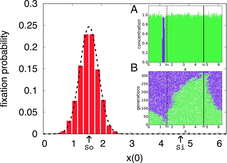
For the case of zero selective advantage, we can analytically compute an approximate fixation probability as a function of position, using a random-walk model. As shown in Fig. 1, simulations are initialized so that only a small, localized window (length or of the interval [0, ] in Fig. 1) contains all of one species. The fixation probability is then measured as a function of the location of this window. By treating these genetic boundaries as random walkers biased by the flow, we find in the limit of small ,
| [6] |
where is the width of the spatial window, is the leftmost genetic boundary, and is the normalized probability density function at , given by a Gaussian with mean and variance . Details are presented in SI Appendix, section D.
Fig. 1.
The fixation probability of an initially localized purple species in a background of green, obtained from 1,000 independent realizations of an agent-based simulation of two neutral populations, as a function of the initial position of the purple distribution. Arrows indicate the locations of the source () and sink (). Populations that begin near the source in the sine wave flow are more likely to fix. The dotted line shows agreement with the random-walk model, Eq. 6, with no fitting parameter. The flow for this plot is . (Inset A) One possible initial condition, with of the domain holding only purple organisms and the rest filled with green organisms. (Inset B) One realization of a fixation event corresponding to the initial condition in Inset A. The dashed line shows the source at and the solid line shows the sink at .
This function defines a length scale for our source, , given by the balance between diffusion and the advecting velocity field. Any organism that can diffuse to the source in a time faster than the source time is relevant to the genetic future of this sine wave system. The farther away an organism is from the source, the stronger the outward velocity field it experiences. Any organism that moves significantly farther than from the source is unlikely to be able to return and has a negligible chance of fixation as it is drawn into the sink.
We hypothesize that for zero or small selective advantage the effective population size scales as the source length scale, times the density of organisms, , which is a constant well approximated by the no-flow limit since we are not in the regime of spatial localization. Based on these considerations, we conclude that
| [7] |
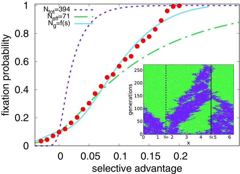
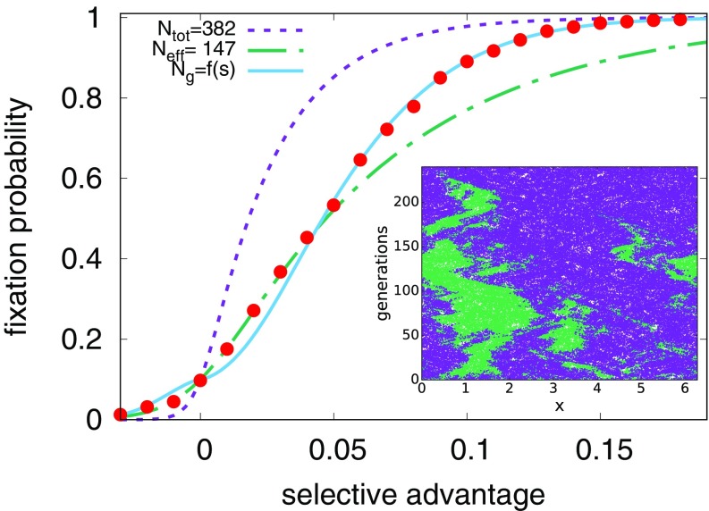
where is a constant of order unity. We see from Fig. 2 that the fixation probability is dramatically different from the case without an external velocity field and is well described by these considerations for small , with . The large difference between () and the total number of organisms in the system () is striking, considering that the presence of the flow cannot be easily detected in the snapshots of the organismic density alone without observing genetic interfaces.
Fig. 2.
The fixation probability (red circles) for an initial condition with a random 10/90 mixture of two species with , varying the selective advantage (, since all organisms are equally likely to take over the population in this limit). The purple line (short dashes) shows Eq. 3, the Kimura no-flow result, for the measured number of organisms in the simulation, . The green line (short and long dashes) gives the prediction of Eq. 7, valid in the limit of small with . The blue line (solid) gives the prediction of Eq. 9 for the large case, with a selective advantage-dependent effective population size. Error bars inferred from 2,000 independent simulations are too small to be visible. (Inset) A single realization for a 50/50 mixture of two neutral species (thus, ). The dashed line marks the position of the source, , and the solid line marks the position of the sink, . Note that the genetic interfaces between purple and green tend to annihilate in the sink at . The total concentration of organisms remains approximately uniform.
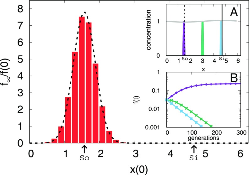
Although a stochastic model was the key to predicting the magnitude of the fixation probability given by Eq. 6, the Gaussian enhancement of the source region is also evident in a purely deterministic model. Deterministic simulations of the neutral case, which directly solve Eqs. 1 and 2 for without number fluctuations, are shown in Fig. 3. Although these simulations, which are equivalent to the agent-based model in the limit , cannot directly observe fixation, we nevertheless see that a small population of one species initially localized close to the source (Fig. 3, Inset A) grows in size until it reaches a steady-state population (Fig. 3, Inset B) more than five times its original size. In contrast, a population starting near the sink shrinks to values that are less than , approximating extinction in a simulation with discrete organisms. A Gaussian with SD centered on the source provides a good fit for Fig. 3, just as in Fig. 1.
Fig. 3.
The final fraction of the initially localized species, , divided by its initial fraction, as a function of its initial location. Populations that begin near the source, (), grow relative to their initial condition, and populations that begin far from the source shrink. Fit is given by a Gaussian of variance . Here , as in Fig. 1. (Inset A) The gray line shows the approximately uniform steady-state total concentration of organisms [the sum of the concentrations of both species, ]. The colored boxes show the initial spatial distribution of one of the species for three different simulations, relative to the source (dashed line) and the sink (solid line). (Inset B) The total fraction of the initially localized species in time, with the colors corresponding to the initial conditions in Inset A. The leftmost initial population prospers, while the middle and rightmost initial populations fall off rapidly.
Strong Selective Advantage with Sine Wave Flows.
When the selective advantage is sufficiently high (although still small compared to 1), it becomes a significant term in Eq. 2 and plays a role in setting the source length. We must now balance the effects of selection, diffusion, and the velocity.
We can do this using the framework of Fisher genetic waves. Consider a species with a significant selective advantage that is sharply localized within a background population, in a system with a sine wave flow with an amplitude that nevertheless satisfies . This initial condition will typically produce two Fisher genetic wavefronts traveling in opposite directions. If the initial population starts on a source, both wavefronts will be supported by the external flow as they move across the system. However, if the initial population starts on a sink, both wavefronts will face an opposing flow.
There is a window of initial conditions around the source at , defined by , where an initial population can produce Fisher genetic waves that deterministically travel across the entire system. Within this window, the flow velocity is small enough that wavefronts can reach the source even if they do not start there. Outside of this window, Fisher genetic waves cannot reach the favorable source region.
Upon treating Fisher waves crossing the system as a proxy for fixation, this argument suggests another way to define an effective population size in the Kimura formula: the number of organisms around the source within the spatial window with boundaries given by .
When we solve for this window, we include a fitting parameter, , because the traveling-wavefront solution occurs only for special initial conditions. The window is then given by half-width such that
| [8] |
After solving for , we can use the approximation of constant density to write the number of organisms in our genetic wave-defined source population as
| [9] |
Note that our effective population size now has dependence. We find that provides good agreement in Fig. 2. At even higher values of selective advantage, where is no longer greater than , we observe a crossover to well-mixed behavior as expected.
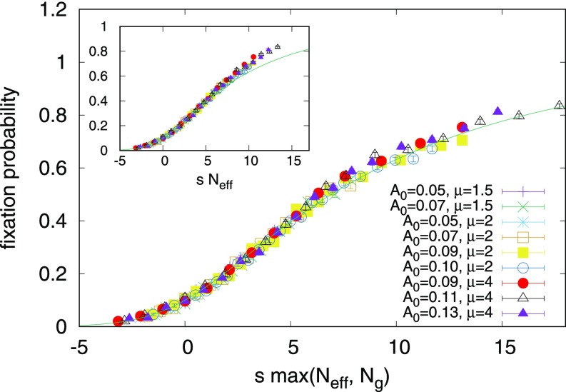
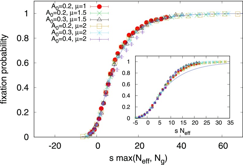
Upon combining these two arguments by using the largest effective population size, , in the original Kimura formula, Eq. 3, we can explain the fixation probability for a weak steady sine wave, as shown in Fig. 4.
Fig. 4.
When we plot the measured fixation probabilities against times the larger effective population size of our two approximations, Eqs. 7 and 9, our data collapse to a master curve. The agreement with our sine wave simulations suggests that we have identified how the fixation varies with and for this parameter regime. Error bars associated with 2,000 independent realizations are shown. for all data points shown, avoiding the crossover to well-mixed behavior seen at high in Fig. 2. (Inset) When plotted as a function of the quasi-neutral theory only, Eq. 7, we see a departure from the theory at high values of , which motivates the high approximation given by Eq. 9.
Turbulent Advection
To generate a 1D chaotic signal with multiscale correlations similar to turbulent flow, we use a well-established set of ordinary differential equations called a shell model (28). For specific details, see ref. 16 and SI Appendix, section E. For the steady sine wave flows studied in the previous section, we saw that the presence of a source can dominate fixation events. It seems reasonable to conjecture that transient, time-dependent sources have a similarly important effect in chaotic turbulent flows and that we can still characterize the system with an effective source dimension and an associated effective population size. Remarkably, we can understand much of the fixation probability with generalizations of the simple theoretical arguments we applied to the stationary sine wave case.
Quasi-Neutral Competitions with Turbulent Advection.
Even in the absence of selection, turbulent dynamics provide new factors to consider when determining the source length scale. The (multiple) sources in the flow can have long or short lifetimes. Their locations move intermittently, and their slopes vary with time. Depending on how the source times compare with the other timescales dictating organism motion, the source-enhanced population at a given time may or may not be able to move with the source and retain its competitive advantage. An example of competitive turbulent dynamics for the neutral case and some further discussion are given in SI Appendix, section F. Although it is clear that understanding the details of fixation probabilities in turbulence is complicated, we can nevertheless apply lessons from the sine wave case to determine scaling behavior.
We assume that our effective population size is the sum of the effective population sizes corresponding to each source, averaged over time. Longer-lived sources thus contribute more to the average and have a greater effect on the effective population size. As in the case of the weakly compressible sine wave, a source’s effective population size should be able to be represented as the density of organisms times a characteristic length. It is not obvious how to define a length for an arbitrary source , but we can easily define a characteristic source time, , by taking the reciprocal of the slope of the positive zero crossing (). Then, we construct a length by assuming the existence of a constant with units of velocity, , that can depend on the diffusion constant and some details of the dynamics, but does not depend on the root mean-square velocity. We can think of as related to the speed with which domain boundaries explore the system.
Therefore, our estimate for in turbulence is
| [10] |
Here, the sum is over all sources present at a given time, and the overbar indicates a time average.
Since the density of organisms, , is approximately constant, it is proportional to , the growth rate. Therefore, we can also understand Eq. 10 as a balance between the organism generation time, , and the source time, . If is large, the generation time is short relative to the source time, and organisms can reproduce many times during the source time. These organisms and their offspring thus experience an enhanced fixation probability, and such sources will give a large contribution to . However, if is small, few organisms are affected, and the contribution to will be small.
We now make the approximation
| [11] |
where is the number of sources and is the root mean-square reciprocal velocity gradient.
We expect that, for a given value of the root mean-square velocity, , the total number of zero crossings, , scales with its gradient. As the root mean-square velocity increases, we expect the number of zero crossings to decrease. These considerations lead to the conjecture
| [12] |
This is known to be true for Gaussian processes in 1D (29), and we have checked it explicitly via simulations with our shell model. A similar relation has been found experimentally in measurements of turbulent flows, where the number of nodes is proportional to the inverse of the Taylor microscale (30).
We note that and are instantaneously strongly fluctuating quantities, and we calculate the dependence of their product on Reynolds number in SI Appendix, section G as . Since this dependence is very weak, we neglect it and make a mean-field approximation to find , where is now time averaged using the harmonic mean.
Upon combining these arguments, and absorbing into the constant , we obtain
| [13] |
Our simulations support this form of as shown in Figs. 5 and 6 with the constant (units of velocity to account for unknown factor) .
Fig. 5.
The fixation probability (red circles) for an initial condition with a random 10/90 mixture of two species advected by a shell model with amplitude and growth rate , for variable selective advantage (). The purple line (short dashes) shows Eq. 3, the no-flow result, for the measured number of organisms in the simulation, . The green line (short and long dashes) gives the prediction of Eq. 7, valid in the limit of small with . The blue line (solid) gives the prediction of Eq. 9 for the large case, with a selective advantage-dependent population size. Error bars inferred from 2,000 independent simulations are too small to be visible. (Inset) A single realization for a 50/50 mixture of two neutral species ().
Fig. 6.
When we plot the measured fixation probabilities against times the larger effective population size of our two approximations, Eqs. 13 and 15, our data collapse to a master curve. The agreement with our shell model simulations suggests that we have identified how the fixation varies with and for this parameter regime. Error bars associated with 2,000 independent realizations are shown. for all data points shown, avoiding the crossover to localized behavior. These parameters ensure that approximate spatial uniformity is maintained. (Inset) When plotted as a function of the quasi-neutral theory only, Eq. 13, we see a departure from the theory at high values of , which motivates the high approximation given by Eq. 15.
Strong Selective Advantage with Turbulent Advection.
As in the sine wave case, we expect a critical value of beyond which selection must be taken into account in the source size calculation. Unlike the quasi-neutral competitions in turbulence, however, we now have an obvious choice for a velocity that can be used to form a length scale—the Fisher genetic wavefront speed. As before, we include a dimensionless fitting parameter, . Our estimate for , the effective population size associated with genetic waves, is
| [14] |
where is the characteristic time of source and the overbar indicates a time average.
Eq. 14 is also the simplest generalization of Eq. 9, obtained by expanding the sine function to linear order in a Taylor series close to each source.
Upon estimating as before, we obtain
| [15] |
This estimate, when in the Kimura formula, Eq. 3, shows good agreement with Figs. 5 and 6, with . As before, we combine the arguments behind Eqs. 13 and 15 by taking the largest effective population size, , in Fig. 6.
Discussion
For both simple (i.e., sine wave) and turbulent compressible flows for which the population density is approximately uniform, we have shown that fixation probabilities are controlled by an effective population size smaller than the total number of organisms in the system in a previously undescribed and biologically relevant region of parameter space. This reduction in the effective population size creates a significant reduction in the fixation probability as a function of selective advantage overall, but a greatly enhanced fixation probability for organisms fortunate enough to be born near sources, even those that are very weak. In the ocean, source regions can be associated with upwellings, if we assume organisms are restricted to live at a certain depth, for example. Our results suggest that the genetic compositions of these regions may have a controlling effect on the genetics of a much greater domain.
Furthermore, we have shown the reduced fixation probabilities can be explained by simple theoretical arguments and can be explored with both agent-based and relatively inexpensive deterministic simulations.
Deviations of Kimura’s formula in the case of strongly compressible turbulence in 1D (i.e., flows that produce spatial localization) have also been observed in simulations, a problem closely related to gene surfing (31).
Supplementary Material
Acknowledgments
We are grateful for the assistance provided by Pinaki Kumar and Francesca Tesser. We thank Amala Mahadevan, Mara Freilich, and Luca Biferale for useful discussions. Work by A.P. and D.R.N. was supported by the National Science Foundation through Grant DMR-1608501 and via the Harvard Materials Science Research and Engineering Center via Grant DMR-1435999. Work by F.T. was partially supported by the Nederlandse Organisatie voor Wetenschappelijk Onderzoek I (NWO-I), The Netherlands.
Footnotes
The authors declare no conflict of interest.
This article is a PNAS Direct Submission.
This article contains supporting information online at www.pnas.org/lookup/suppl/doi:10.1073/pnas.1812829116/-/DCSupplemental.
References
- 1.d’Ovidio F, De Monte S, Alvain S, Dandonneau Y, Lévy M. Fluid dynamical niches of phytoplankton types. Proc Natl Acad Sci USA. 2010;107:18366–18370. doi: 10.1073/pnas.1004620107. [DOI] [PMC free article] [PubMed] [Google Scholar]
- 2.Lévy M, Jahn O, Dutkiewicz S, Follows MJ, d’Ovidio F. The dynamical landscape of marine phytoplankton diversity. J R Soc Interf. 2015;12:20150481. doi: 10.1098/rsif.2015.0481. [DOI] [PMC free article] [PubMed] [Google Scholar]
- 3.Prairie JC, Sutherland KR, Nickols KJ, Kaltenberg AM. Biophysical interactions in the plankton: A cross-scale review. Limnol Oceanogr Fluids Environ. 2012;2:121–145. [Google Scholar]
- 4.Lévy M, Ferrari R, Franks PJ, Martin AP, Rivière P. Bringing physics to life at the submesoscale. Geophys Res Lett. 2012;39:L14602. [Google Scholar]
- 5.Clayton S, Nagai T, Follows MJ. Fine scale phytoplankton community structure across the Kuroshio front. J Plankton Res. 2014;36:1017–1030. [Google Scholar]
- 6.Clayton S, Dutkiewicz S, Jahn O, Follows MJ. Dispersal, eddies, and the diversity of marine phytoplankton. Limnol Oceanogr Fluids Environ. 2013;3:182–197. [Google Scholar]
- 7.De Monte S, Soccodato A, Alvain S, d’Ovidio F. Can we detect oceanic biodiversity hotspots from space? ISME J. 2013;7:2054–2056. doi: 10.1038/ismej.2013.72. [DOI] [PMC free article] [PubMed] [Google Scholar]
- 8.Wares JP, Pringle JM. Drift by drift: Effective population size is limited by advection. BMC Evol Biol. 2008;8:235. doi: 10.1186/1471-2148-8-235. [DOI] [PMC free article] [PubMed] [Google Scholar]
- 9.Chust G, Irigoien X, Chave J, Harris RP. Latitudinal phytoplankton distribution and the neutral theory of biodiversity. Glob Ecol Biogeogr. 2013;22:531–543. [Google Scholar]
- 10.Giovannoni SJ, Stingl U. Molecular diversity and ecology of microbial plankton. Nature. 2005;437:343–348. doi: 10.1038/nature04158. [DOI] [PubMed] [Google Scholar]
- 11.Krieger MS, McAvoy A, Nowak MA. Effects of motion in structured populations. J R Soc Interf. 2017;14:20170509. doi: 10.1098/rsif.2017.0509. [DOI] [PMC free article] [PubMed] [Google Scholar]
- 12.Herrerías-Azcué F, Pérez-Muñuzuri V, Galla T. Stirring does not make populations well mixed. Sci Rep. 2018;8:4068. doi: 10.1038/s41598-018-22062-w. [DOI] [PMC free article] [PubMed] [Google Scholar]
- 13.Whitlock MC. Fixation probability and time in subdivided populations. Genetics. 2003;164:767–779. doi: 10.1093/genetics/164.2.767. [DOI] [PMC free article] [PubMed] [Google Scholar]
- 14.Behrenfeld MJ, et al. Climate-driven trends in contemporary ocean productivity. Nature. 2006;444:752–755. doi: 10.1038/nature05317. [DOI] [PubMed] [Google Scholar]
- 15.Pigolotti S, Benzi R, Jensen MH, Nelson DR. Population genetics in compressible flows. Phys Rev Lett. 2012;108:128102. doi: 10.1103/PhysRevLett.108.128102. [DOI] [PubMed] [Google Scholar]
- 16.Benzi R, Nelson DR. Fisher equation with turbulence in one dimension. Phys D Nonlinear Phenom. 2009;238:2003–2015. [Google Scholar]
- 17.Kimura M. On the probability of fixation of mutant genes in a population. Genetics. 1962;47:713–719. doi: 10.1093/genetics/47.6.713. [DOI] [PMC free article] [PubMed] [Google Scholar]
- 18.Maruyama T. A simple proof that certain quantities are independent of the geographical structure of population. Theor Popul Biol. 1974;5:148–154. doi: 10.1016/0040-5809(74)90037-9. [DOI] [PubMed] [Google Scholar]
- 19.Perlekar P, Benzi R, Nelson DR, Toschi F. Population dynamics at high Reynolds number. Phys Rev Lett. 2010;105:144501. doi: 10.1103/PhysRevLett.105.144501. [DOI] [PubMed] [Google Scholar]
- 20.Pigolotti S, et al. Growth, competition and cooperation in spatial population genetics. Theor Popul Biol. 2013;84:72–86. doi: 10.1016/j.tpb.2012.12.002. [DOI] [PubMed] [Google Scholar]
- 21.Jacox MG, Hazen EL, Bograd SJ. Optimal environmental conditions and anomalous ecosystem responses: Constraining bottom-up controls of phytoplankton biomass in the California current system. Sci Rep. 2016;6:27612. doi: 10.1038/srep27612. [DOI] [PMC free article] [PubMed] [Google Scholar]
- 22.Bravo L, Ramos M, Astudillo O, Dewitte B, Goubanova K. Seasonal variability of the Ekman transport and pumping in the upwelling system off central-northern Chile (∼ 30° S) based on a high-resolution atmospheric regional model (WRF) Ocean Sci. 2016;12:1049–1065. [Google Scholar]
- 23.Pollard R, Regier L. Vorticity and vertical circulation at an ocean front. J Phys Oceanography. 1992;22:609–625. [Google Scholar]
- 24.Moore L. Comparative physiology of Synechococcus and Prochlorococcus: Influence of light and temperature on growth, pigments, fluorescence and absorptive properties. Mar Ecol Prog Ser. 1995;116:259–275. [Google Scholar]
- 25.Hallatschek O, Korolev K. Fisher waves in the strong noise limit. Phys Rev Lett. 2009;103:108103. doi: 10.1103/PhysRevLett.103.108103. [DOI] [PubMed] [Google Scholar]
- 26.Doering CR, Mueller C, Smereka P. Interacting particles, the stochastic Fisher-Kolmogorov-Petrovsky-Piscounov equation, and duality. Phys A Stat Mech Appl. 2003;325:243–259. [Google Scholar]
- 27.Hartl DL, Clark AG. Principles of Population Genetics. Sinauer Associates; Sunderland, MA: 1997. [Google Scholar]
- 28.Biferale L. Shell models of energy cascade in turbulence. Annu Rev Fluid Mech. 2003;35:441–468. [Google Scholar]
- 29.Rice S. Mathematical analysis of random noise. In: Wax N, editor. Selected Papers on Noise and Stochastic Processes. Dover Publications; New York: 1955. pp. 133–294. [Google Scholar]
- 30.Kailasnath P, Sreenivasan K. Zero crossings of velocity fluctuations in turbulent boundary layers. Phys Fluids A Fluid Dyn. 1993;5:2879–2885. [Google Scholar]
- 31.Hallatschek O, Nelson DR. Gene surfing in expanding populations. Theor Popul Biol. 2008;73:158–170. doi: 10.1016/j.tpb.2007.08.008. [DOI] [PubMed] [Google Scholar]
Associated Data
This section collects any data citations, data availability statements, or supplementary materials included in this article.


