Abstract
Advances in high-throughput imaging allow researchers to collect three-dimensional images of whole organ microvascular networks. These extremely large images contain networks that are highly complex, time consuming to segment, and difficult to visualize. In this paper, we present a framework for segmenting and visualizing vascular networks from terabyte-sized three-dimensional images collected using high-throughput microscopy. While these images require terabytes of storage, the volume devoted to the fiber network is ≈ 4 percent of the total volume size. While the networks themselves are sparse, they are tremendously complex, interconnected, and vary widely in diameter. We describe a parallel GPU-based predictor-corrector method for tracing filaments that is robust to noise and sampling errors common in these data sets. We also propose a number of visualization techniques designed to convey the complex statistical descriptions of fibers across large tissue sections—including commonly studied microvascular characteristics, such as orientation and volume.
Keywords: Microvessel, network tracking, glyph visualization, predictor-corrector, segmantation, spherical harmonics, superquadrics, KESM
1. INTRODUCTION
FIBERS and filaments, often connected into large networks, are frequently encountered in biomedicine. Examples include microvascular vessels, or microvessels, that are visible using magnetic resonance angiography (MRA) [1] or computed tomography angiography (CTA) [2]. Microvascular networks, formed by complex interconnected microvessels, play a key role in brain tissue function [3], [4]. Microvascular structures are also commonly studied in cancer, where tumors emit signaling proteins that encourage microvessel growth [5]. The important role of microvessels in disease makes them a strong target for clinical intervention [6]. However, researchers and clinicians do not fully understand the characteristics of microvascular networks and how they can be used to diagnose disease or quantify treatment.
Recent advances in high-throughput microscopy, such as Knife-Edge Scanning Microscopy (KESM) [7], allow fast acquisition of large, terabyte sized data sets at microscopic resolution [8], [9] for understanding complex microvascular structures. The resulting images are terabytes in size and challenging to reconstruct, since they are extremely thin and tortuous. The shear volume of data demands efficient, automated, and scalable algorithms that are robust to noise and can be run in a medical and research setting. However, the highly interconnected nature of these networks makes the development of a robust segmentation framework challenging. Existing methods [10], [11], [12] typically involve constant user intervention during the fiber segmentation, which greatly limits their scalability. This paper attempts to address this scalability issue while improving the segmentation accuracy.
Once the microvascular networks are extracted, visualizing and interpreting their complex structure is necessary for experts to diagnose and compare networks. Among many characteristics, the anisotropy property of features in structures, composed of filament data, is of particular interest to domain specialists. Pathologists, for example, can use anisotropy measures in microvascular data to quantify and categorize structural changes due to the development of certain diseases such as Alzheimer’s (Fig. 2). However, due to the space filling and highly interconnected nature of the networks, it is nearly impossible to parse the anisotropy property of certain characteristics of the networks from the conventional visualization techniques, such as the direct volume rendering as shown in Fig. 3. In particular, it is difficult to answer questions regarding anisotropic features, including
What is the general direction of the fibers in this region?
Are the fibers in this region homogeneous or heterogeneous in nature?
Are these two regions the same in terms of the fibers in them?
These questions are difficult to answer because visually human eyes tend to focus on outliers and attribute more importance to them than to other parts of the visualization that may be more important. In the case of microvascular data, this is demonstrated in Fig. 3 where the thick fibers might be given higher importance, when in reality the thinner fibers are more in numbers and contribute more to blood flow in the closed system. This reduces an expert’s ability to quantitatively distinguish and compare densely connected networks. Solving this issue is one of the primary motivators for this work.
Fig. 2.
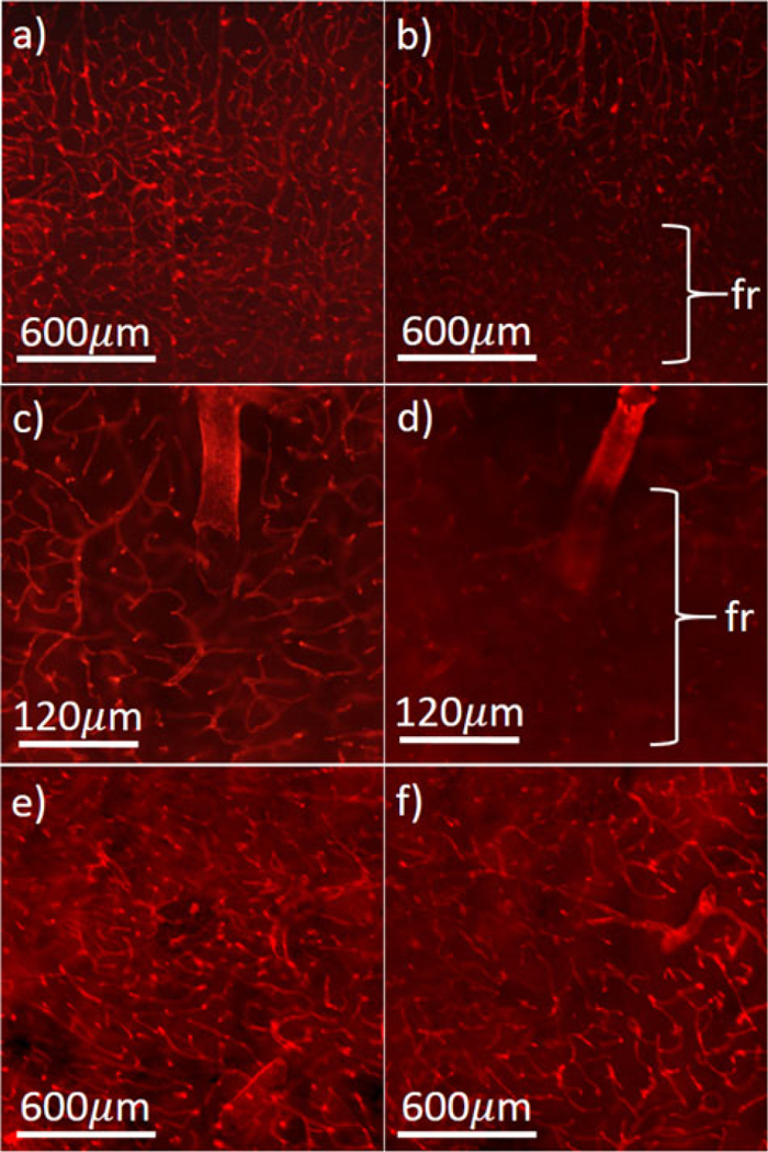
Heterogeneity in microvessel structure. Examples of mouse microvessels stained using Collagen IV antibody, from age-matched wild-type (a) and 12-month-old APdE9 (Alzheimer’s Disease) (AD) models (b). Close-ups show vessel sparsity and fragmentation (fr) in the AD model (c-d). Structural variations are also seen in different brain regions, including caudoputamen (e) and basolateral amygdaloid nucleus (f).
Fig. 3.
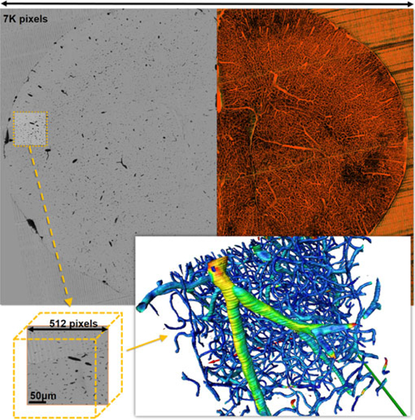
KESM image of a mouse brain (top left) shown as a maximum intensity projection over 1,000 slices (top right). The total depth of the image stack is 7,000 slices. Traditional approaches rely on extracting a sub-volume (bottom left) to generate an iso-surface for visualization (bottom right). Here, color mapping is based on vessel radius. As the volume size increases, the visualization quickly becomes GB to interpret.
To address the above challenges, we present researchers and pathologists with a scalable framework to segment dense microvascular networks and to visualize important anisotropic characteristics of the extracted networks that can be used for analysis and comparison between regions in heterogeneous tissue samples. In particular, we make the following two major contributions in this work.
We revisit the formulation of a template-based predictor-corrector algorithm [12] (Section 3) to optimize the segmentation algorithm by reducing the required number of samples (Section 3.2), and by introducing a novel and automated branch detection process (Section 4);
We devise strategies to effectively visualize aggregated anisotropy information about the aforementioned segmented networks that are useful to experts (Section 5). In particular, we employ the binning technique to aggregate a number of statistical information of the network so that glyphs can be applied to visualize this aggregated information in a concise form. Specifically, we describe the mathematical model for fitting 2nd-order symmetric tensors to the anisotropic directionality information to enable a visualization using superquadric tensor glyphs. In addition, we model the distribution of various statistics information of the fibers within a local region using the spherical harmonics, which enables us to visualize this high-order information using high-order glyphs. In this work, we focus on two primary metrics: flow-distance and flow-volume, where flow-distance is based on the length of decomposed microvessels and in flow-volume the decomposed microvessels are weighted by their volume. For both metrics we assume the direction of flow to be ambiguous.
While we focus our implementation (see a publicly available link in the Appendix, which can be found on the Computer Society Digital Library at http://doi.ieeecomputersociety.org/10.1109/TVCG.2018.2818701) on microvascular data and demonstrate how our methods can be of use to pathologists and researchers interested in the effects of certain diseases, these methods and strategies can be adapted to other disciplines where cylindrical structures are common.
2. RELATED WORK
In this section, we will discuss current work in the areas of microvascular segmentation, specifically focusing on algorithms that are practical for terabyte-scale data sets. We will then discuss work in visualizing and characterizing network structures.
2.1. Network Segmentation and Fiber Tracking
Standard methods used to collect 3D images of microvascular networks rely on confocal microscopy [13], [14], which is generally limited to 200–300 mm thick sections. While more advanced techniques can alleviate depth constraints [15],[16], they do so at the expense of image acquisition time. In order to collect large volumes of tissue, our analysis is performed on data obtained using Knife-Edge Scanning Microscopy [7].
Many algorithms are effective for the segmentation of MRA and CTA [17], where vessels are large (≈ 1 mm) and form tree-like structures. Traditional MRA and CTA images are also significantly smaller, making time-consuming pat-tern recognition algorithms more practical. Microvessels,on the other hand, are often ≈ 4 μm in diameter and no more than a few pixels in size. In addition, KESM data that contain miscrovessels are typically with terabyte size, which demands data-parallel approaches using GPU-based hard-ware to process [18].
A majority of algorithms focus on image pre-processing to isolate larger blood vessels [19], [20]. While multi-scale techniques can be used to accelerate this pre-processing, most microvessels have the same small diameter at or near the sampling rate, resulting in little improvement. Methods based on selecting threshold values, such as centerline detection [21] and thinning [22] work well on small, high-contrast data sets. For large-scale data sets, these thresholds tend to vary significantly and require iterative pixel-level processing. Such methods are also susceptible to artifacts. KESM offers relatively high signal-to-noise ratio (SNR), but the process suffers from barding, striping and staining arti-facts [12] as shown in Fig. 1. During segmentation these arti-facts are responsible for topological errors as well assignificant over-segmentation. Region growing approaches[23] are effective for segmenting vessel surfaces, but require a relatively complex initial surface which can be difficult to find in the complex topology of the network. Convolutional neural networks (CNN) are shown to be effective at dealing with sampling noise, dropped fibers and cyclical data [24]at the cost of extra time spent on training.
Fig. 1.
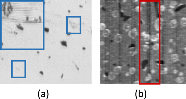
A cropped section of two different KESM data sets using different stains: India-Ink (a) and Thionin (b) collected using KESM. Poor staining can lead to a loss of fibers (blue), while striping can lead to over002dsegmentation (red), our algorithm was tested on both of these data sets.
Template matching methods [10] are robust, at the high computational cost of matching templates with multiple ori-entations and scales, even if the majority of the voxels contain no relevant fiber information. Vector tracking methods[11] share some similarity to template matching, but rely on an underlying vector field to simulate particle advection for tracking fiber paths. The bottleneck in both cases is sampling, which becomes time-consuming for large data sets. GPU-based tracking methods offer a solution by parallelizing data fetches [12]. However, these methods require constant user-intervention in the form of (manual) seed-point selection. In practice, an automated approach is desired.
In this paper, we implement a robust GPU tracking algorithm that (a) significantly reduces the number of samples required in the previous work [12] and (b) uses prior information about network connectivity to eliminate the need for user intervention but allows the user to tune the algorithm to prioritize performance and/or accuracy.
2.2. Microvascular Morphology
Microvascular morphology varies significantly across organs and tissue types (Fig. 2). There is extensive research exploring the statistical and morphological variations in microvascular structures, most prominently in the brain [13], [14]. Models produced using images of microvasculature have been used to understand flow characteristics [25], [26]. This research plays a critical role in understanding the neurovascular unit, a biological concept that couples microvessels with surrounding neurons [27], [28]. These structures may have a significant effect on disease progression and are candidates for many translational treatments [29]. Microvasculature also plays an important role in tumor growth [30], where antiangiogenic therapy is a critical component in treatment [31]. Finally, there is significant evidence for microvascular variation in neurodegenerative disease and psychiatric disorders [32], many of which can be used to quantify the effectiveness of treatment using pharmaceuticals [33].
2.3. Visualization
All of these afformentioned analyses rely on accurate characterization of microvascular networks, which are extremely difficult to quantify. This is primarily due to two factors: (a) limited ability to collect large volumes of data describing microvascular structures and (b) inability to explore how microvascular structures vary across multiple regions or samples. Visualization offers a tangible solution to help experts analyze and characterize these networks.
Standard visualization techniques (e.g., direct volume rendering and iso-surfacing) may be useful for understanding small volumes. For instance, direct volume rendering methods are useful for selective fiber visualization that focuses on visualizing culled and partial volumes (Fig. 2). Jeong et al. propose a similar method for segmentation and visualization of large tubular structures [34]. However, their method focuses on visualizing a few fibers. It is unclear whether their approach can provide a clear visualization of dense and highly interconnected networks, as we are dealing with in this work. In practice, volume rendering and iso-surfacing for the networks at the scale necessary to understand micro-vascular morphology are difficult to interpret (Fig. 3). Other methods have used the graph-like structure of networks in order to selectively visualize network features [35]. This allows raw volumetric data to be visualized using highly compressed structures, such as OpenVDB [36], [37] that build a correlation between the volumetric data and a connected graph.
Most of the aforementioned existing visualization techniques focus on the exploration of specific physical structures. In contrast, our goal in this work is to convey to researchers how the statistical properties of the sub-networks vary within a large heterogeneous microvascular network. We focus on using local functions, in the form of tensor fields and spherical harmonics, and glyphs to convey local, aggregated network characteristics. Ropinski et al. conduct a survey of glyph-based visualization techniques for bio-medical data [38], including diffusion tensor imaging, diffusion weighted MRI, and CT based data. In contrast, we focus on making use of the extensive work on glyph-based tensor visualization [39], [40], [41] to handle dense and complex microvascular networks in this work. We aim to demonstrate that these matured glyph-based techniques (e.g., superquadric glyph) for DTI data are equally useful for visualizing summarized vascular information and conveying the necessary information.
3. NETWORK TRACKING
We are given a 3D data set representing a grayscale image with an intensity difference between pixels that lie inside and outside of the network. We assume that the network is highly connected, i.e., any given volume contains very few disconnected components. Reconstructing the network from requires:
tracing one filament given a seed location
identifying points where filaments branch or connect
generating new seed locations as necessary
Given an initial seed point, we track the corresponding fiber using a predictor-corrector algorithm [11], which calculates the movement of a tracer along the filament path. Each tracer has the following properties:
-
1)
position on the network
-
2)
estimated trajectory of the fiber at p
-
3)
estimated size
Given a tracer at any point on the network, we update the component values using a predictor-corrector algorithm to obtain (Algorithm 1). The tracer is initialized at a seed point i = 0 and terminates when a stopping condition is met. In order to optimize data look-ups, a GPU-based algorithm is used to parallelize memory fetches [12].
Algorithm 1.
Predictor-Corrector Algorithm Used to Segment a Single Microvessel
| Require: (p0, v0, s0) |
| Ensure: a list P = [p0,...,pn] |
| a list S = [s0,...,sn] |
| i = 0 |
| while terminating conditions are not met do |
| vi+1 = Predict (pi+1, vi, si) |
| pi+1 = Correct (vi, si) |
| si+1 = Fit (pi+1, vi+1) |
| i = i + 1 |
| end while |
| DetectBranches |
In the following Section 3.1 we outline the mathematical model used for template matching. We then propose several modifications from previous algorithms to significantly reduce the number of required samples for cost function computation (Section 3.2). In Sections 3.3, 3.4, 3.5, and 3.6 we describe the individual steps of our predictor-corrector algorithm. Finally, Section 4 describes our new, automated branch-detection method.
3.1. Template Matching
The center of any shape embedded in an implicit function can be found by specifying a cost function C based on the integral of absolute differences between the image and a template function that matches the desired shape
| (1) |
where
is a position vector in some pre-defined template space such that and is an augmented affine transformation matrix used to transform points from the template space to coordinates in Any arbitrary position, orientation, and/or scale can be evaluated by specifying T using a single template f. The optimal transformation matrix is found by minimizing the cost function
| (2) |
This optimization will find a set of transformation matrices such that
| (3) |
where all pi lie at the medial axis of the network. Note that calculating directly is a high-dimensional (16-D), optimization, which is impractical for large images. In order to address this we isolate the optimization to the minimal template required to identify the shape.
3.2. Cost Function Sampling
The template function f is typically symmetric. In our work, we opt for a cylindrical template function symmetric about (and independent of) the z-axis
| (4) |
Thus, f depends only on the and components (Fig. 4), resulting in the simplified cost function
| (5) |
Fig. 4.
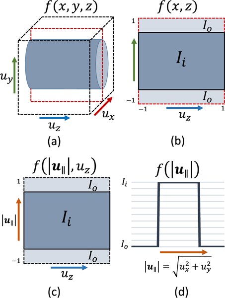
Simplification of 3D volumetric template matching to a 2D integral with a 1D template. (a) The entire template is shown, with the coordinates given in a consistent template space. Cross-sections of the template are shown along the y(b) and x(c) axes. Note that the template at are identical (d), while the template function itself can be expressed as a 1D function of distance from
Consider a two-dimensional slice through the center of (Fig. 4a)
| (6) |
If a symmetric fiber is aligned with the cost function can be approximated by integrating the volume of revolution
| (7) |
However, a single template cross-section is insufficient to guarantee that the central template coordinate lies at the fiber center, since any cylindrical cross section oriented along will produce a matching pattern (Fig. 4c). Two cross-sections are therefore required to ensure correct localization of the vessel center line, resulting in a pair of two-dimensional cost functions used to approximate the volumetric result (Fig. 4d)
| (8) |
| (9) |
| (10) |
This allows us to approximate a cylindrical fit by minimizing two orthogonal 2D integrals, rather than a single 3D integral as is previously proposed [12]
| (11) |
3.3. Predict—Estimate Fiber Orientation
Given a position and size of tracer an estimate of the fiber trajectory vi is calculated. To find the optimal direction vector we choose a series of N unit vectors uniformly distributed within a solid angle [12].
For each vector we create a transformation matrix that aligns the template function to the current tracer position pi, with size si and along the candidate orientation Evaluating the cost function (Equation (10)) for each candidate vector produces a set of corresponding cost values where corresponds to the direction of the tracer (Algorithm 1).
3.4. Correct—Estimate Fiber Medial Axis
Based on the position and orientation of the current tracer an initial guess p′ of the next tracer position is estimated using Euler’s method
| (12) |
where is the update step size This position is then corrected by sampling a uniform set of N points on the plane orthogonal to and within distance from A transformation matrix is calculated for each candidate point using orientation and scale . The point corresponding to the minimum cost value (Equation (10)) is used for the new tracer position (Algorithm 1).
3.5. Fit—Estimate Fiber Size
The final step adjusts the scale parameter of the tracer to obtain a better fit to the fiber. The new scale value is estimated by sampling M uniformly with samples Corresponding transformation matrices are generated using the position and orientation After evaluating the cost function for all samples, is set to the scale value associated with the minimum (Algorithm 1).
3.6. Termination Conditions
The functions Predict(·), Correct(·), and Fit(·) (Algorithm 1) continue until one of four conditions is satisfied:
C(T) > λ where λ is a maximum cost value allowed for a successful template match.
pi goes outside of the bounds of the image Г.
The tracer intersects a previously segmented filament.
If the size of the template changes too quickly over a short number of steps.
The most used termination conditions are (3) intersecting a previously traced vessel and (2) hitting the boundary of the traceable volume. Encountering the case where C(T) > λ is generally due to an image or tissue preparation artifact. In the case of India ink perfusion [42], this artifact may be a bubble in the dye or a burst vessel. If λ is properly calibrated, this condition is rarely triggered. This threshold will be much smaller than the maximum possible cost. For example if both the image and template are normalized: .
Condition (3) for termination is critical for reconstructing network connectivity. Intersections are detected during tracing using a nearest-neighbor search. If an intersection is identified, tracing is terminated and the network connectivity is updated (see Appendix, available in the online supplemental material).
The last condition is used as a failsafe to stop segmentation in areas of poor staining, where the microvessel becomes indistinguishable from the background. In this case the FIT step will choose the largest size of the template to maximize the difference between the template and the sample. This signals that the algorithm has lost track of the microvessel, and the segmentation from the current seed point is then terminated.
4. BRANCH DETECTION
When a termination condition is satisfied, our algorithm automatically looks for potential seed points. This process is called branch detection. Note that there is no automatic branch detection in the previous method [12]. Since the network is highly connected, we expect candidates to be adjacent to the traced fiber defined by centerline and radii found by the Fit and Correct functions (Algorithm 1).
We first parametrize the surface surrounding the fiber as a 2D manifold that forms a generalized cylinder around the centerline P, where the distance between and the closest point on R is proportional to si (Fig. 5). We establish this parameterization by creating four continuous functions used to build a local, rotation minimizing Frenet frame using a quaternion to avoid orientation flips [43]:
: continuous centerline for the fiber
: local tangent to the centerline
: normal vector
: radius of R
Fig. 5.
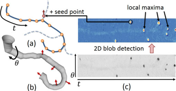
The vessel centerline (a) is used to define a 2D manifold R that takes the form of a generalized cylinder (b). This cylinder is unwrapped into a flat image (c, bottom). Candidate seeds are found using LoG blob detection (c, top). These candidate seed points in are mapped back into Cartesian coordinates in Г. Their initial orientation v0 is given by the associated normal to R (red arrows). These serve as the starting state for candidate fibers.
The intensity value of any point on the surface can be calculated using
| (13) |
where x is the position of is the surface normal of R. In our implementation are piecewise linear functions generated from P and S, respectively using linear interpolation. The derivative function is calculated using finite differences along P. Finally, the normal is the result of a quaternion transformation from an initial arbitrary orientation perpendicular to All functions are continuous along the interval
To find the locations of candidate seed points, we use Laplacian of Gaussian (LoG) blob detection by finding the local maxima of the separable convolution
| (14) |
Candidate seed points are placed at the corresponding 3D location in Г (Equation (13)). The initial fiber direction v0 = v (Equation (13)) is the surface normal at R.
We implemented the above segmentation and network construction framework using GPUs. The implementation details of those critical steps, such as sampling, cost function evaluation and branch point detection are provided in the Appendix, available in the online supplemental material. A reference implementation (with source code) can be accessed via a link provided in the Appendix, available in the online supplemental material.
5. VISUALIZATION
After applying the above segmentation and network tracking algorithm to the input data, large and complex micro-vascular networks are obtained. As discussed earlier, direct volume rendering or iso-surfacing (Fig. 3) of such networks cannot effectively convey important biological information. To address that we instead focus on aggregating and visualizing multimodal statistical information regarding a number of important characteristics of microvascular networks, such as blood flow volume and vessel orientation. The following strategies also work on other statistical features important to biologists as long as they can be decomposed into a vector representation. We employ two strategies to generate the visual representation for the aggregated information. First, based on the extracted vessels and their directional information we fit a second-order symmetric positive definite (s.p.d) tensors, from which superquadric glyphs are constructed to convey the general trends of the vessel orientation. Second, we estimate the distribution of the directional information of the fibers within a local region (e.g., a data block of the entire data set) using spherical histograms, based on which we fit a spherical harmonic function to create a glyph. This glyph enables the representation of the aggregated multimodal vessel characteristics represented by the shape and other statistics using a projected colormap on the glyph. Both strategies preserve the multimodality of the underlying distributions, a necessity for distinguishing between regions. In the following we provide more details on these two visualization strategies.
5.1. Anisotropic Statistics
Vessel orientation or directionality is of particular interest when attempting to differentiate two networks [44], or when creating artificial (synthesized) microvascular networks that are statistically similar to real tissues. Such an artificial microvasculature is important for understanding the physiological properties of red blood cells [45] and tissue fabrication [46]. Visualizing directionality information is a complex endeavor as the network cannot be represented by a continuous vector field (Fig. 3) and the local propagation trend is not clearly identifiable using volume rendering.
In order to extract the directional information, we decompose every vessel into a collection of vectors. Any given vessel can be decomposed into n − 1 segments, each of which is defined as pi−pi+1. Given this decomposition we are now able to analyze statistics associated with directional information. Flow volume, for example, is a scaling of the directional information relative to the size of the vessel. This can be quite unintuitive to visualize because the thicker vessels need not carry the larger flow since the microvasculature is much more dense.
To demonstrate the presence anisotropy, we bin each segment according to its direction in spherical coordinates to create a spherical histogram. To account for ambiguous flow direction, each vector is binned along with it’s inverse. We project the resulting histogram onto the surface using both color mapping and deformation (Fig. 6).
Fig. 6.
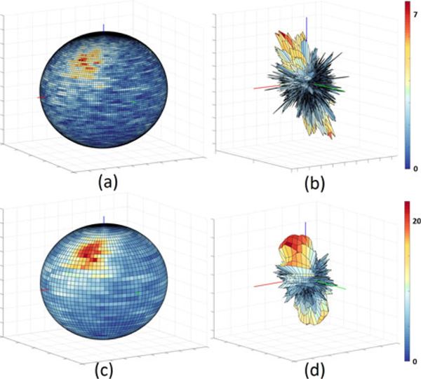
The results of binning decomposed vessels and projecting them onto a sphere (left) as well as using them to create a surface (right). Color is mapped to the number of vectors in each bin. While using a large number of bins preserves details (a)-(b), aggregating the bins highlights any pattern present in the vessel decomposition (c)-(d). The ranges are subdivided into 90 and 180 bins (top), respectively, and aggregated into 45 and 90 bins (bottom). In order to deal with the varying bin size we divide the contents of each bin by its calculated size (integral over the volume of the bin). Note the reduction in the number of artifacts as the bin size increases. All binning figures are symmetric since every vector and its inverse are binned, to account for ambiguous blood flow direction.
The resulting histogram provides an overview of the orientation of microvessels. Many regions in normal tissue have highly oriented microvessels, while others are isotropic. The histogram also suggests that the orientation can be multimodal. Because of this heterogeneity and multimodality, researchers attempt to quantify vessel orientation in order to characterize tissue [13], generally using 1D angular histograms. In the following sections, we describe two strategies for visualizing this aggregated anisotropic information of the network, both of which employ the glyph representations to achieve an abstract visualization while using different mathematical models to map the anisotropic information to glyphs.
5.2. Superquadrics
The spherical histograms discussed in the previous section, while precise in visualizing the directional details of a single tissue section, are not particularly effective for larger heterogeneous samples where multiple histograms would be useful to capture the changing statistics. Spherical histogram representations only convey directional information and its visualization quality depends purely on perspective, while the surface deformations lack uniformity and consistency in shape (Fig. 6). The histogram’s ability to display heterogeneity is achievable with glyphs, which are commonly used for tensor and vector field visualization. In what follows, we describe a glyph representation to convey the aggregated directional statistics within a local region. Our first strategy resorts to superquadrics to represent the above aggregated information. In particular, we place glyphs within the individual data blocks, which allows us to obtain an overview of fiber directions for a large heterogeneous data sets as well as their change due to locality.
In this work we chose to represent vessel flow-distance (G0) and flow-volume (G1), because they are generally considered both biologically useful for pathologist classifying blood vessel degenerative diseases, as well as neurological models used in fields, such as fMRI, and are difficult to characterize using traditional visualization methods. The local information for both of these quantities can be encoded in a tensor
| (15) |
| (16) |
where Vi is the volume of a frustum made from two circles of radius sn and sn+1. The flow-volume tensor is similar to the flow-distance tensor, however thick microvessels have a significantly larger effect in this representation. Due to the nature of the superquadric representation we are still able to visualize sections of tissue with microvessels propagating in multiple directions.
For each cube of data we create a single tensor representation using the above formulation. Due to the symmetric nature of the problem, we only keep 6 of the 9 entries for each tensor in a cube. For tissue blocks composed of multiple sections we stitch the tensor representations into a rectilinear grid and export the resulting binary file for visualization using Amira [48]. The results of this visualization technique for a 2 × 9 × 1 grid of 5123 pixels is shown in Fig. 7 with intermediate values being interpolated.
Fig. 7.
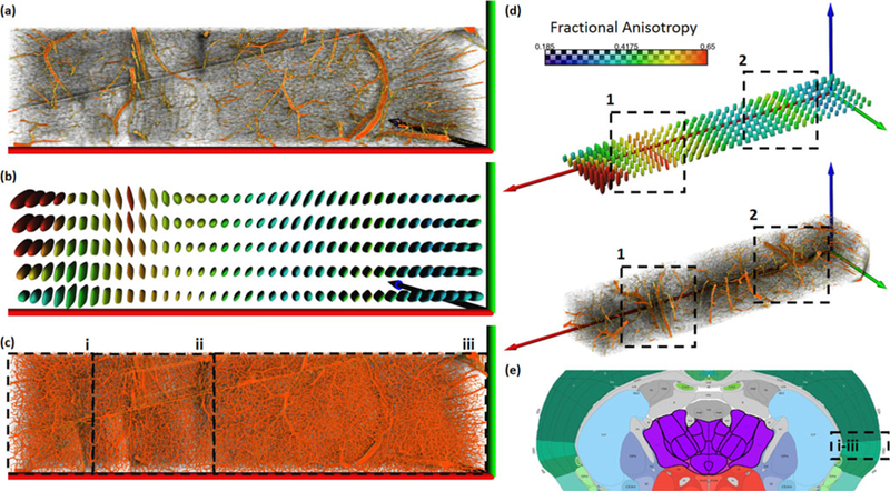
Result visualization from a large section of segmented tissue (inset-e) using superquadrics from several perspectives. The region is composed of multiple brain regions including caudoputamen (CP) (i), corpus colossum and supra-colossal white matter (ccb/scwm) (ii), and the cortical surface (iii). We present resampled data showing large vessels (a) and the actual data (c) visualized using MIP. Glyphs (b and d) show the directed volume of blood flow and are colored based on fractional anisotropy [47]. The volume tensor demonstrates the ability to extract larger trends present in the data, such as in region (2) (in (d)) where a color variation reveals the presence of a large central blood vessel, and perpendicular branching in the cortical tissue. This is further exemplified in CP (1) where a few large vessels heavily affect the shape of the glyphs. We note that in (2), the density of the vessels is much higher than in (1), which lessens the effects of large vessels. As seen by variations in glyph shape and size (b), superquadrics allow the user to visualize spatially varying trends in vascular orientation within the region.
5.3. Spherical Harmonics
Superquadrics are well understood in visualization, however the statistical distributions of features like flow volume and flow direction are not clearly conveyed due to their multimodality. In order to achieve a visual representation of the mean and variance of these anisotropic features, we use spherical harmonics (SH) [49] to generate smoothed spherical functions capturing these distributions.
To find a set of SH coefficients that best represents the overall directionality, we consider all of the decomposed vessels in a segmented region as a set of measurements where si scales the directional segments in spherical coordinates. Each scale si is weighted by the length of the segment described by and a weight wi which is calculated by
| (17) |
where k is some scaling factor. The contribution of is higher if are parallel with a perpendicular vector contributing nothing. The model function is a spherical harmonic of order L given by
| (18) |
where is the formulation of spherical harmonic functions of the order l and degree m.
In order to align the functions with the direction of the fibers we use the tesseral spherical harmonics. The real form is given by
| (19) |
| (20) |
where is the associated Legendre polynomial. For the rest of the formulation we will be using the 1D index We define the least squares cost function as the difference between the model function and each sample sn as
| (21) |
where Note that the cost function K(c) is quadratic in terms of coefficients meaning there is only one minimum in the first derivative. We minimize the cost function by setting the first derivative dk/dc to 0 and simplifying
| (22) |
Equation (22) yields a linear system of equations that we can solve for all cj in This solution represents the spherical harmonic that optimally fits the samples in S.
We used a Python implementation [50] to directly compute as well as solve the linear system of equations. A large value of N provides higher accuracy, while a large value of L provides sharper features and a closer fit to the histograms as presented in Figs. 6b and 6d. However, this can result in overfitting, with a lobe around every sample if the number of samples is too small. The number of samples required to accurately model the underlying distribution increases exponentially as a factor of L, which is the main limitation of the algorithm. Aside from this limitation spherical harmonic glyphs offer all the same advantages as their superquadric counterparts, including interpolation. Typically for a network consisting of 50,000 samples, an appropriate choice for L is 100, i.e the degree of the spherical harmonic basis equaling to 9. The set S is typically composed of all the fibers in a particular segmentation blocks. The scaling factor k is chosen to be 200 in our simulations.
Since each individual harmonic is created for a smaller sub-volume composing a larger tissue section and the sub-volumes are uniformly spaced, we form a rectilinear grid. The colormaps in Fig. 8 are also calculated as a spherical harmonic. The volume of each fiber segment is calculated as a conical frustum and stored as a separate set of coefficients, meaning that each point in the rectilinear grid is composed of two spherical harmonics, one representing the shape of the glyph, another representing the colormap for that glyph. As described in Equation (20) each harmonic is stored as a set of coefficients multiplied by static functions, meaning that by storing the numerical coefficients we can interpolate between functions on our rectilinear grid. Since the colormap is an independent spherical harmonic, we can also interpolate between two color harmonics.
Fig. 8.
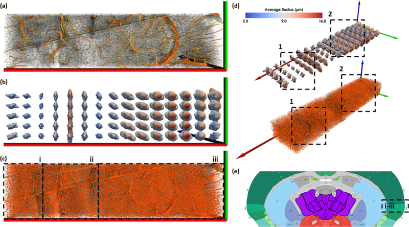
Visualization of a large section of segmented tissue (e) using spherical harmonic (SH) glyphs from several perspectives. The visualized data covers multiple brain regions, including CP (i), ccb/scwm (ii), and the cortical surface (iii). We present resampled data showing large vessels (a) and the actual data (c) visualized using MIP. Glyphs (b and d) use two colormaps. (b) When the color map corresponds to the shape of the spherical function, the highlighted directions indicate the direction of longer vessels. (d) Alternatively, basing the colormap on vessel radius indicates the prominent directions of blood flow. In this case, the glyph shape and colormap indicate two different features: the glyph shape indicates vessel volume/direction, while the glyph color indicates vessel radius/direction. The size of the glyphs correlates with the density of the microvasculature in the region, as seen by the difference is density between regions (1) and (2). At the cost of complexity and size, SH glyphs are better than superquadrics at showing anisotropy and connectivity. The ccb/scwm (ii) is surrounded by smaller glyphs on the left and right, signifying a small amount of microvasculature connecting the structure to CP (i) and the cortical surface (iii), which is biologically true. Furthermore, the shape of the SH glyphs highlight the anisotropic characteristics of the microvascular network, such as in the cortical surface (2) where the vessels are more homogeneous in growth when compared the structure in region (1), where the vessels tend toward the y/z-plane, further supporting that the ccb/scwm structure is microvascularly separable from it’s neighbors in this area.
6. RESULTS AND DISCUSSION
In this section, we report the results of our segmentation and visualization framework, along with an expert evaluation (Section 6.1). To quantitatively assess performance, we report the average timing of the segmentation process (Section 6.2) and study its accuracy (Section 6.3) by comparing our method with the previous methods. Finally, we perform a parameter study to assess the stability of our algorithm, which provides users a guidance on selecting appropriate input parameters for their specific data (Section 6.4).
6.1. Evaluation
We have applied the proposed algorithms to several data sets visualized using superquadric (Fig. 7) and spherical (Fig. 8) glyphs, respectively. These results were submitted to domain experts for comments. The review process was composed of a short tutorial in which we explained the visualization mapping. The tutorial was composed of Fig. 9, demonstrating the resulting glyphs encoding the summarized characteristics for different microvascular networks. Following this explanation we allowed the experts to conduct their visual analysis without interference, and asked them specific questions regarding homogeneity and heterogeneity of the regions represented by our visualization. Each glyph was shown first without the accompanying maximum intensity projection (MIP) image. High resolution and low resolution MIP images were shown afterwards, allowing experts to validate their comments and to gain additional insights. Visualizations were shown in the following order:
-
1)
Tutorial image (Fig. 9)
-
2)
200 × 3000 × 200 micron tissue section visualized using superquadrics (Figs. 7b and 7d)
-
3)
the accompanying high and low-resolution maximum intensity projections (Figs. 7a, 7c, and 7d)
-
4)
a 200 × 3000 × 200 micro section visualized using spherical harmonic glyphs (Fig. 8c)
-
5)
the MIP of the same region (Fig. 8b).
Fig. 9.
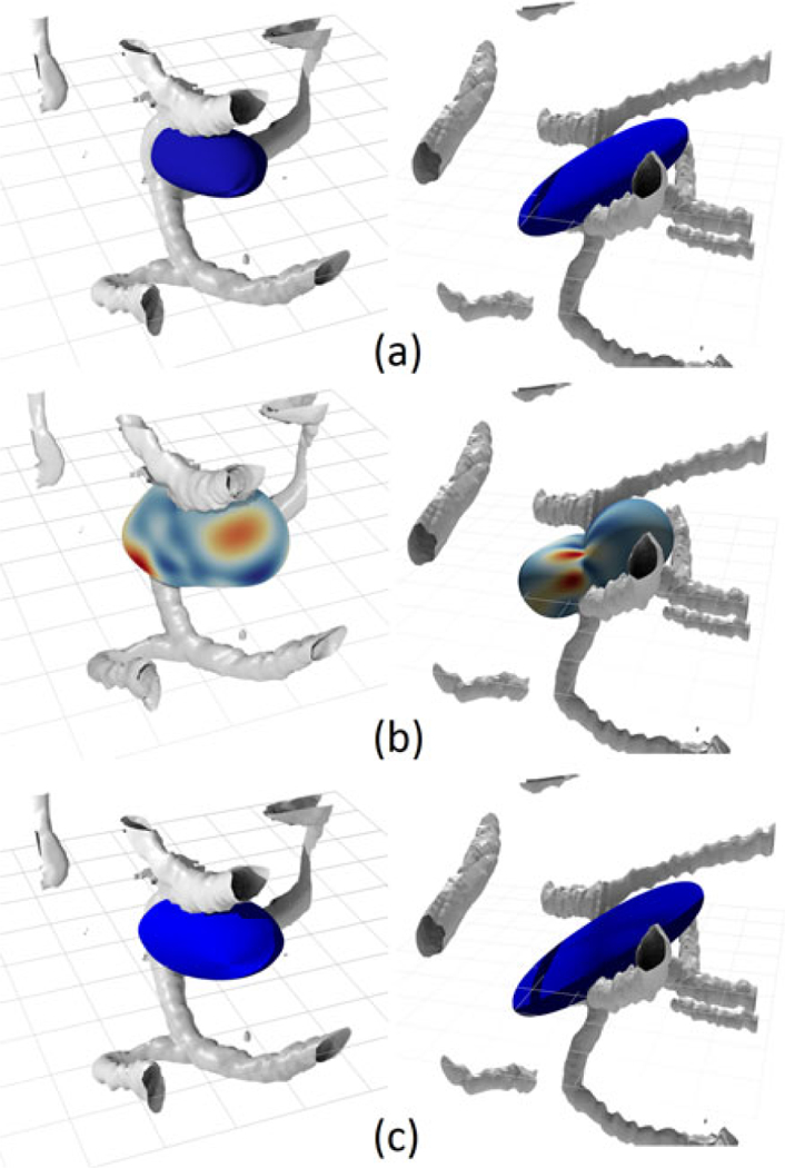
To demonstrate the viability of both the spherical harmonics and the superquadrics we display some cases of both used to represent small networks with only a few fibers (a, b, c). From top to bottom are length-direction superquadric, a spherical harmonic with an average radius color map and flow-volume superquadric superimposed over small number of segmented fibers (grey). We show two types of networks, a more homogeneous case (left) and a more heterogeneous case (right). The harmonic is generate with l = 8 and N = 100k. The network on the left contains fibers with relatively constant radii and the network on the right contains fibers of varying radii. All three cases are presented at optimal viewing angles for demonstrating the shapes of the glyphs relative to the network. The color maps for such small network on the spherical harmonic surfaces tend to be quite sparse due to a smaller number of fibers. In these sparse cases they represent the actual direction of propagation of fibers. The volume and direction superquadrics are much better at representing the bi-directional modality common in these mini-networks. The distinct difference between the volume (c) and the length (a) glyphs is a direct result of the presence of fibers with varying radii. This difference is a lot less prominent in a more homogeneous network.
Using the superquadrics visualization (Fig. 7b), experts were able to easily discriminate between normal and transgenic mice, since the flow was “of a consistent orientation” in control animals. They were also able to ascertain that there were three regions represented in the brain: (1) caudoputamen (Fig. 7c-i), (2) white matter (Fig. 7c-ii), (3) and cortical surface (Fig. 7c-iii). In addition, the experts found that the “visual 744 flow could be used to select regions for further analysis and could be used to extract information about underlying structures,” such as in the caudoputamen. They were able to select regions of interest based on their homogeneity and heterogeneity. As for the MIP image (Fig. 7c), Expert 1 indicated that it was difficult to identify a predominant direction of the fibers due to the vascular density. The MIP images tend to draw the attention of the viewer to the large vessels, however, “seeing the large vessels is not as important since the majority of pathological vascular changes are associated with alterations in capillary structures in these models”. One limitation of both the MIP images and the superquadric glyphs indicated by our experts is that the quality of analysis was dependent on the view perspective that was presented.
When presented with the spherical glyph visualization (Fig. 8c), the experts noted that they preferred the spherical harmonic representation over the the superquadric approach. Specifically, spherical harmonics provided “a clearer visual representation of the homogeneity and heterogeneity of the capillary structure, while showing the position of the larger vessels that exist perpendicular to the capillaries” than using superquadrics. The experts agreed that the “information represented by the superquadrics and spherical harmonics appears to be similar to the MIP images but that the spherical harmonics approach simplified the detection of microvascular heterogeneities, and offered clearer representation of vascular microvasculature flow”; however, both experts mentioned that they would need the MIP to provide more content for the analysis. After seeing the accompanying maximum intensity projection, one expert said that “with enough training it would be viable to analyze the data without the MIP”. They did, however, mention that it would be useful to have the superquadric visualization as “a supplement to the MIP”.
6.2. Timing
The algorithm performs well. Tables 1 and 2 provide the timing information of our segmentation algorithm tested on a section of tissue with 512 × 512 × 300 pixels in size containing fibers. Table 1 shows the breakdown of the performance on the individual steps of our algorithm, while Table 2 shows the averaged per fiber segmentation time over every fiber in a 3.7 Gb India Ink data set and a 6.7 Gb Thionin data set respectively. The total segmentation time of the India Ink data is 1.6 hours, and 2.8 hours for the Thionin data set. The time spent per cube is difficult to average since the actual performance depends on the number of fibers inside each individual volume rather than the size of the data. Hence, Table 2 is a better representation of the timing. Compared to Mayerich’s approach [12], our new segmentation algorithm achieves about 50 percent speedup in total performance (Table 1), while our method is about 10x faster than Mayerich’s approach in the predict and correct steps and at least 3x faster in other steps (Table 2). The most time consuming stage of our segmentation is the collision detection. The amount of time spent on rendering the entire network to detect collisions increases as more fibers are segmented. This is due to the current collision detection framework implemented via OpenGL selection mode, which we plan to improve in the future.
TABLE 1.
Timing Breakdown of the Total Segmentation Time
| Our approach (India Ink) |
Mayerich’s approach (India Ink) [12] |
Our approach (Thionin) |
|
|---|---|---|---|
| Total Time | 16.975 s | 30.462 s | 20.323 s |
| Predict step | 1.484 s | unreported | 0.869 s |
| Correct step | 1.449 s | unreported | 0.858 s |
| Fit step | 1.429 s | unreported | 0.807 s |
| Cost calculation | 1.678 s | unreported | 3.340 s |
| Branch detection | 0.507 s | unreported | 0.729 s |
| Collision detection | 9.682 s | unreported | 13.720 s |
TABLE 2.
Step Breakdown (Average Performance)
| Our approach (Nissl and India Ink) |
Mayerich’s approach [12] |
|
|---|---|---|
| Cost calculation | 67.40 ns/step. | 0.230 ms/step |
| Predict Step | 0.123 ms/step. | 1.248 ms/step |
| Correct Step | 0.122 ms/step. | 1.177 ms/step |
| Fit Step | 0.121 ms/step. | 0.994 ms/step |
6.3. Accuracy
To evaluate the accuracy of our method, we manually segmented the aforementioned test volume Г using a simple application we developed specifically for that purpose. The program allows a user to cycle through the image stack composing Г and click on the approximate center of each fiber at the location in the image stack. This process was used to segment every fiber and was repeated multiple times with differences in results merged in order to achieve complete accuracy. The resulting volume was rechecked again to make sure the tissue block was completely segmented. Connectivity information was ignored since the extracted point where one fiber merges with the other was often difficult to distinguish. The fiber was simply ended in the location where two fibers start merging, since this area is clearly distinguishable for every fiber merging, resulting in approximate connectivity information. This may cause a slightly higher False Positive Rate (FPR) error in areas where the fibers interconnect. The algorithm showed a high accuracy as compared to manual segmentation: 4.769 percent FPR and and False Negative Rate (FNR) of 8.054 percent. The FNR statistic is of significant importance as it shows where the algorithm fails to detect the fibers. The areas of error are generally located in the corners and the edges of the volume, where fibers from adjacent volumes enter, but do not connect to the main network. Because each execution of our algorithm uses a single seed point, the algorithm will only find the interconnected fibers. Any fibers at the edge of the volume that enter and exit without connecting to the main bulk of fibers are invisible to the segmentation algorithm. This can be alleviated by adding multiple seed points, one for every fiber at the edge of the volume T using an LoG filter, a process similar to branch detection. The results in Fig. 10 show both the regions with high error that are heavily localized to the edge of the volume. We hypothesize that the majority of these can be removed by using multiple seeds.
Fig. 10.
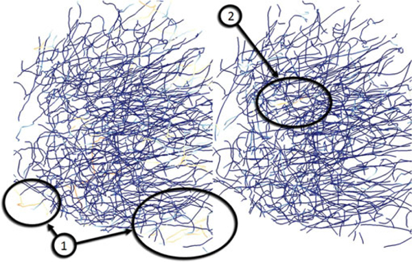
A comparison of the manually traced network (left) and the predictor-corrector algorithm (right) using a single initial seedpoint. All brightly colored fibers on the left represent fibers present in the manual segmentation but absent in the predictor-corrector results contributing to the false-negative ratio (FNR), while bright fibers on the right are present in the automated segmentation but absent in the manual segmentation increasing the false positive ratio (FPR). Majority of the fibers found during manual segmentation are also present in the automatically segmented network. The major contributors to the FNR are the fibers on the edge of the network that are not connected to the central network.
Another source of error is due to bad staining. Regions of a poorly stained fibers that become indistinguishable from the background for a significant length cause the algorithm to terminate. While using the manual segmentation tool, the user can easily predict where the fiber is based on where it becomes indistinguishable and where it continues, in most cases this distance is only a few pixels in length, which is still enough for the algorithm to lose track. Such staining artifacts result in an inflation of the FNR ratio.
Our algorithm does miss some fibers that are not a result of border issues. These tend to be exceptionally small fibers interconnecting with thicker vessels. When the fiber has a large radius during the branch-detection phase, smaller interconnections on the surface of the larger fiber are lost due to under sampling. In most case, these lost fibers are handled when another fiber of similar radius connects with them at a different point. In cases when the prior condition is not met those fibers are lost permanently. Large fibers may occasionally cause errors, specifically around thick fibers where the tracer may segment the same large fiber multiple times and artificially creates a connection to a neighboring fiber of similar thickness (2). This can possibly be avoided by implementing collision detection using cylinders, instead of line segments. Mayerich et al., did not report accuracy in their work.
We performed the segmentation and timing using NVidia GTX 1080 GPU and an Intel i7–5820K CPU and 32 GB of RAM under Ubuntu 16.04. During testing we found that the type of processor did not have an noticeable effect on the performance. RAM was also not the limiting fact since the majority of the memory allocation is isolated to the GPU. Additionally the algorithm was tested and timed on other GPU configurations including: NVidia GTX 1070, Nvidia Titan X, and Nvidia GeForce 700 with no noticeable performance difference. The choice for using the Nvidia GeForce 700 was to compare with the hardware available during the publication of the previous paper [12].
6.4. Parameter Study
In this section we study how various parameters in our algorithm affect the result on KESM data. As with Lagrangian particle advection, the most important parameter is Δτ, which in our implementation is set directly by tweaking the parameter δ. In our algorithm the parameter δ is constrained by Values above 1 are not recommended as it would advance the tracer across regions of the data set that have not been sampled. While setting a smaller can increase the accuracy of the segmentation, it may lead to oversampling, hence adversely affecting the performance. We chose for all the tracing performed in this work, as it achieves a good trade-off between accuracy and performance.
Another important parameter to consider is the sampling resolution (i.e., the size of the templates in terms of pixel resolution). This parameter has very little effect in the plane, but is important in the plane (i.e., along the filament), especially for noisy data. A larger value provides smoother integration along the filament length, and therefore a higher accuracy in noisy data sets with the cost of more computation time on sampling and cost evaluation. We chose values that are multiples of 8 to maximize the occupancy in the CUDA-based cost evaluation (see Appendix, available in the online supplemental material, for more details). For high contrast data a parameter of 8 is often adequate. However, because the cost and evaluation processes of the algorithm are relatively cheap we found that using 16 px produced the best result, while values higher than 16 px did not result in a significant increase in accuracy for our KESM data sets, an example of which was shown in Fig. 3.
The last parameters that we studied are the numbers of templates for direction, correction and fitting. An advantage to using the predictor-corrector algorithm is the high tolerance for inaccuracies. Any error in the direction prediction is corrected during the later steps, for that reason the number of direction templates is generally kept high, while the number of correction templates is kept much lower. The cost on sampling is still relatively small compared to other stages of the algorithm, but in general we found that the ratio 1/0.5/0.25 for Predict/Correct/Fit is most ideal for our data sets. One thing to keep in mind is the size of the texture that the GPU can handle. We tested values of 1,000, 500, 250 and 100, and we found that keeping the value of 250 was optimal for tracing the entire network. Setting larger values resulted in unnoticeable increase in accuracy, at the cost of oversampling and a slight decrease in performance.
The cost value is a user-selected parameter, but has no influence to the performance. This parameter needs to be tuned for every specific data set. The maximum value depends on the sampling resolution and the template type. For a uniform template of size 16 the maximum value is 256, considering that the sampled data is complete opposite of the template. For the KESM data set this algorithm was tested on the value between 190 and 200, and we chose 198 for the best results. This value was used across the entire data set and not only the sub-volume displayed previously. For glyph visualization we used 100,000 samples to create the spherical harmonics.
7. CONCLUSION AND FUTURE WORK
Our main goal is to provide an efficient network tracking framework to address the increasing abundance of large high-throughput microscopy data sets. We also present a number of glyph-based visualization techniques to represent the aggregated, biologically relevant information of the extracted network to aid the inspection and comparison of these complex networks. This is an important problem for researchers exploring the statistical and morphological variations in microvasculature, but lack the tools to do so efficiently. We apply our segmentation and visualization techniques to a large data set obtained using KESM to demonstrate their efficacy. Our aggregation strategies for generating glyphs using spherical harmonics, superquadrics and binning, present statistical information about large interconnected microvascular networks embedded in tissue. We show that our techniques are robust enough to reduce the amount of visualized data without losing detail about local and global microvascular trends.
There are a number of limitations to the current approach. First, our framework is currently implemented using an OpenGL/CUDA inter-operability framework, which might not be optimal. We plan to further improve the performance by performing all sampling in CUDA or to explore the recent release of Vulkan by the Kronos group [51]. Second, our visualization strategies remove most information about the connectivity of individual microvessels, while the segmentation portion of our toolset retains connectivity information. In the future, we plan to use layout generation algorithm and clustering algorithms to enable the exploration of the networks as graph structures.
Supplementary Material
ACKNOWLEDGMENTS
This work is supported in part by the Cancer Prevention and Research Institute of Texas (CPRIT) #RR140013, National Institutes of Health/National Library of Medicine #4 R00 LM011390–02, National Institutes of Health/National Cancer Institute #1R21CA21 4299–01, and US National Science Foundation (IIS 1553329).
Biography
 Pavel A. Govyadinov is working toward the graduate degree in the Department of Computer Science, University of Houston. His research focuses on visualization and reconstruction of large data sets obtained using high-throughput microscopy. He is a student member of the IEEE.
 Tasha Womack is working toward the graduate degree in the Department of Pharmacology, University of Houston. Her research focuses on the imaging and quantification of blood vessels in Alzheimer’s disease models using three-dimensional microscopy.
 Jason L. Eriksen is an associate professor with the Department of Pharmacology, University of Houston. His research focuses primarily on histology and microvascular staining, with a particular focus on neurovascular changes that occur in Alzheimer’s disease.
 Guoning Chen received the PhD degree in computer science from Oregon State University, in 2009. He is an assistant professor with the Department of Computer Science, University of Houston. Before joining the University of Houston, he was a post-doctoral research associate with the Scientific Computing and Imaging Institute, University of Utah. His research interests include visualization, data analysis, computational topology, geometric modeling, geometry processing, and physically-based simulation. He is a member of the IEEE and ACM.
 David Mayerich received the PhD degree in computer science from Texas A&M University and worked as a Beckman postdoctoral fellow with the University of Illinois at Urbana-Champaign. He is an assistant professor with the Department of Electrical and Computer Engineering, University of Houston. His research focuses on high-throughput imaging of brain and cancer tissue, as well as high-performance computing for analyzing large datasets. He is a member of the IEEE.
Contributor Information
Pavel A. Govyadinov, Department of Computer Science, University of Houston, Houston, TX 77031..
Tasha Womack, Department of Pharmacological and Pharmaceutical Sciences, University of Houston, Houston, TX 77031.
Jason L. Eriksen, Department of Pharmacological and Pharmaceutical Sciences, University of Houston, Houston, TX 77031.
Guoning Chen, Department of Computer Science, University of Houston, Houston, TX 77031..
David Mayerich, Department of Electrical and Computer Engineering, University of Houston, Houston, TX 77031..
REFERENCES
- [1].Dumoulin CL and Hart H Jr, “Magnetic resonance angiography,” Radiol, vol. 161, no. 3, pp. 717–720,1986. [DOI] [PubMed] [Google Scholar]
- [2].Hulten EA, Carbonaro S, Petrillo SP, Mitchell JD, and Villines TC, “Prognostic value of cardiac computed tomography angiography: A systematic review and meta-analysis,” J. Amer. College Cardiology, vol. 57, no. 10, pp. 1237–1247, 2011. [DOI] [PubMed] [Google Scholar]
- [3].Farrall AJ and Wardlaw JM, “Blood-brain barrier: Ageing and microvascular disease-systematic review and meta-analysis,” Neurobiol. Aging, vol. 30, no. 3, pp. 337–352, 2009. [DOI] [PubMed] [Google Scholar]
- [4].Brown WR and Thore CR, “Review: Cerebral microvascular pathology in ageing and neurodegeneration,” Neuropathology Appl. Neurobiol, vol. 37, no. 1, pp. 56–74, 2011. [DOI] [PMC free article] [PubMed] [Google Scholar]
- [5].Carmeliet P and Jain RK, “Angiogenesis in cancer and other diseases,” Nature, vol. 407, no. 6801, pp. 249–257, 2000. [DOI] [PubMed] [Google Scholar]
- [6].Jain RK, “Normalization of tumor vasculature: An emerging concept in antiangiogenic therapy,” Sci, vol. 307, no. 5706, pp. 58–62, 2005. [DOI] [PubMed] [Google Scholar]
- [7].Mayerich D, Abbott L, and McCormick B, “Knife-edge scanning microscopy for imaging and reconstruction of three-dimensional anatomical structures of the mouse brain,” J. Microscopy, vol. 231, no. 1, pp. 134–143, 2008. [DOI] [PubMed] [Google Scholar]
- [8].Pepperkok R and Ellenberg J, “High-throughput fluorescence microscopy for systems biology,” Nature Rev. Mol Cell Biol, vol. 7, no. 9, pp. 690–696, 2006. [DOI] [PubMed] [Google Scholar]
- [9].Glory E and Murphy RF, “Automated subcellular location determination and high-throughput microscopy,” Develop. Cell, vol. 12, no. 1, pp. 7–16, 2007. [DOI] [PubMed] [Google Scholar]
- [10].Sato Y, Nakajima S, Shiraga N, Atsumi H, Yoshida S, Koller T,Gerig G, and Kikinis R, “Three-dimensional multi-scale line filter for segmentation and visualization of curvilinear structures in medical images,” Med. Image Anal, vol. 2, no. 2, pp. 143–168, 1998. [DOI] [PubMed] [Google Scholar]
- [11].Al-Kofahi KA, Lasek S, Szarowski DH, Pace CJ, Nagy G, Turner JN, and Roysam B, “Rapid automated three-dimensional tracing of neurons from confocal image stacks,” IEEE Trans. Inf. Technol. Biomed, vol. 6, no. 2, pp. 171–187, Jun. 2002. [DOI] [PubMed] [Google Scholar]
- [12].Mayerich D and Keyser J, “Hardware accelerated segmentation of complex volumetric filament networks,” IEEE Trans. Vis. Comput. Graph, vol. 15, no. 4, pp. 670–681, Jul./Aug. 2009. [DOI] [PubMed] [Google Scholar]
- [13].Lauwers F, Cassot F, Lauwers-Cances V, Puwanarajah P, and Duvernoy H, “Morphometry of the human cerebral cortex microcirculation: General characteristics and space-related profiles,”Neuroimage, vol. 39, no. 3, pp. 936–948, 2008. [DOI] [PubMed] [Google Scholar]
- [14].Cassot F, Lauwers F, Lorthois S, Puwanarajah P, Cances-Lauwers V, and Duvernoy H, “Branching patterns for arterioles and venules of the human cerebral cortex,” Brain Res, vol. 1313, pp. 62–78, 2010. [DOI] [PubMed] [Google Scholar]
- [15].Tsai PS, Friedman B, Ifarraguerri AI, Thompson BD, Lev-Ram V, Schaffer CB, Xiong Q, Tsien RY, Squier JA, and Kleinfeld D, “All-optical histology using ultrashort laser pulses,” Neuron, vol. 39, no. 1, pp. 27–41, 2003. [DOI] [PubMed] [Google Scholar]
- [16].Ragan T, Kadiri LR, Venkataraju KU, Bahlmann K, Sutin J, Taranda J, Arganda-Carreras I, Kim Y, Seung HS, and Osten P, “Serial two-photon tomography for automated ex vivo mouse brain imaging,” Nature Methods, vol. 9, no. 3, pp. 255–258, 2012. [DOI] [PMC free article] [PubMed] [Google Scholar]
- [17].Rudyanto RD, Kerkstra S, Van Rikxoort EM, Fetita C, Brillet P-Y, Lefevre C, Xue W, Zhu X, Liang J, I. (Oksiiz, et al. , “Comparing algorithms for automated vessel segmentation in computed tomography scans of the lung: The VES-SEL12 study,” Med. Image Anal, vol. 18, no. 7, pp. 1217–1232, 2014. [DOI] [PMC free article] [PubMed] [Google Scholar]
- [18].Smistad E, Falch TL, Bozorgi M, Elster AC, and Lindseth F, “Medical image segmentation on GPUs-A comprehensive review,” Med. Image Anal, vol. 20,no.1,pp.1–18,2015. [DOI] [PubMed] [Google Scholar]
- [19].Yu Z and Bajaj C, “A segmentation-free approach for skeletonization of gray-scale images via anisotropic vector diffusion,” in Proc. IEEE Comput. Society Conf. Comput. Vis. Pattern Recognit, 2004, pp. I-415–I-420. [Google Scholar]
- [20].Zhang Y, Bazilevs Y, Goswami S, Bajaj CL, and Hughes TJ, “Patient-specific vascular NURBS modeling for isogeometric analysis of blood flow,” Comput. Methods Appl. Mech. Eng, vol. 196, no. 29, pp. 2943–2959, 2007. [DOI] [PMC free article] [PubMed] [Google Scholar]
- [21].Tozaki T, Kawata Y, Niki N, Ohmatsu H, Eguchi K, and Moriyama N, “Three-dimensional analysis of lung areas using thin slice CT images,” in Proc. SPIE Conf. Medical Imaging, 1996, pp.2–11. [Google Scholar]
- [22].He X, Kischell E, Rioult M, and Holmes TJ, “Three-dimensional thinning algorithm that peels the outmost layer with application to neuron tracing,” J. Comput.-Assisted Microscopy, vol. 10, no. 3, pp. 123–135,1998. [Google Scholar]
- [23].O’Brien JF and Ezquerra NF, “Automated segmentation of coronary vessels in angiographic image sequences utilizing temporal, spatial, and structural constraints,” in Proc. SPIE Vis. Biomed. Comput, 1994, pp. 25–37. [Google Scholar]
- [24].Wang S, Yin Y, Cao G, Wei B, Zheng Y, and Yang G, “Hierarchical retinal blood vessel segmentation based on feature and ensemble learning,” Neurocomput, vol. 149, pp. 708–717, 2015. [Google Scholar]
- [25].Gagnon L, Smith AF, Boas DA, Devor A, Secomb TW, and Sakadzic S, “Modeling of cerebral oxygen transport based on in vivo microscopic imaging of microvascular network structure, blood flow, and oxygenation,” Frontiers Comput. Neurosci, vol. 10, p. 82, 2016, [DOI] [PMC free article] [PubMed] [Google Scholar]
- [26].Schmid F, Tsai PS, Kleinfeld D, Jenny P, and Weber B, “Depth-dependent flow and pressure characteristics in cortical microvascular networks,” PLoS Comput. Biol, vol. 13, no. 2, 2017, [DOI] [PMC free article] [PubMed] [Google Scholar]
- [27].Hawkins BT and Davis TP, “The blood-brain barrier/neurovascular unit in health and disease,” Pharmacological Rev, vol. 57, no. 2, pp. 173–185, 2005. [DOI] [PubMed] [Google Scholar]
- [28].Zlokovic BV, “Neurodegeneration and the neurovascular unit,” Nature Med, vol. 16, no. 12, pp. 1370–1371, 2010. [DOI] [PubMed] [Google Scholar]
- [29].McConnell HL, Kersch CN, Woltjer RL, and Neuwelt EA, “The translational significance of the neurovascular unit,” J. Biol. Chemistry, vol. 292, no. 3, pp. 762–770, 2017. [DOI] [PMC free article] [PubMed] [Google Scholar]
- [30].Ehling J, Theek B, Gremse F, Baetke S, Mockel D, Maynard J, Ricketts S-A, Grull H, Neeman M, Knuechel R, et al. , “Micro-CT imaging of tumor angiogenesis: Quantitative measures describing micromorphology and vascularization,” Amer. J. Pathology, vol. 184, no. 2, pp. 431–441, 2014. [DOI] [PMC free article] [PubMed] [Google Scholar]
- [31].Ye W, “The complexity of translating anti-angiogenesis therapy from basic science to the clinic,” Develop. Cell, vol. 37, no. 2, pp. 114–125, 2016. [DOI] [PubMed] [Google Scholar]
- [32].Katsel P, Roussos P, Pletnikov M, and Haroutunian V, “Microvascular anomaly conditions in psychiatric disease. Schizo-phrenia-angiogenesis connection,” Neurosci. Biobehavioral Rev, vol. 77, pp. 327–339, 2017. [DOI] [PMC free article] [PubMed] [Google Scholar]
- [33].Udristoiu I, Marinescu I, Pirlog M-C, Militaru F, Udristoiu T, Marinescu D, and Mutica M, “The microvascular alterations in frontal cortex during treatment with antipsychotics: A post-mortem study,” Romanian J. Morphology Embryology, vol. 57, no. 2, pp. 501–506,2016. [PubMed] [Google Scholar]
- [34].Jeong W-K, Beyer J, Hadwiger M, Vazquez A, Pfister H, and Whitaker RT, “Scalable and interactive segmentation and visualization of neural processes in EM datasets,” IEEE Trans. Vis. Comput. Graph, vol. 15, no. 6, pp. 1505–1514, Nov./Dec. 2009. [DOI] [PMC free article] [PubMed] [Google Scholar]
- [35].Mayerich D, Abbott L, and Keyser J, “Visualization of cellular and microvascular relationships,” IEEE Trans. Vis. Comput. Graph, vol. 14, no. 6, pp. 1611–1618, Nov./Dec. 2008. [DOI] [PubMed] [Google Scholar]
- [36].Museth K, “VDB: High-resolution sparse volumes with dynamic topology,” ACM Trans. Graph, vol. 32, no. 3, 2013, [Google Scholar]
- [37].Balme J, Brown-Dymkoski E, Guerrero V, Jones S, Kessler A, Lichtl A, Lung K, Moses W, Museth K, Roberson N, et al. , “Extreme multi-resolution visualization: A challenge on many levels,” 2015. [Google Scholar]
- [38].Ropinski T, Oeltze S, and Preim B, “Survey of glyph-based visualization techniques for spatial multivariate medical data,” Com put. Graph, vol. 35, no. 2, pp. 392–401, 2011. [Google Scholar]
- [39].Kindlmann G, “Superquadric tensor glyphs,” in Proc. 6th Joint Eurographics-IEEE TCVG Conf. Vis, 2004, pp. 147–154. [Google Scholar]
- [40].Zhang C, Schultz T, Lawonn K, Eisemann E, and Vilanova A, “Glyph-based comparative visualization for diffusion tensor fields,” IEEE Trans. Vis. Comput. Graph, vol. 22, no. 1, pp. 797–806, Jan. 2016. [DOI] [PubMed] [Google Scholar]
- [41].Seltzer N and Kindlmann G, “Glyphs for asymmetric second-order 2D tensors,” Comput. Graph. Forum, vol. 35, no. 3, pp. 141–150, 2016. [Google Scholar]
- [42].Xue S, Gong H, Jiang T, Luo W, Meng Y, Liu Q, Chen S, and Li A, “Indian-ink perfusion based method for reconstructing continuous vascular networks in whole mouse brain,” PLoS One, vol. 9, no. 1, 2014, [DOI] [PMC free article] [PubMed] [Google Scholar]
- [43].Shoemake K, “Animating rotation with quaternion curves,” ACM SIGGRAPH Comput. Graph, vol. 19, no. 3, pp. 245–254,1985. [Google Scholar]
- [44].Mayerich D, Bjornsson C, Taylor J, and Roysam B, “NetMets: Software for quantifying and visualizing errors in biological network segmentation,” BMC Bioinf., vol. 13, no. 8, 2012, [DOI] [PMC free article] [PubMed] [Google Scholar]
- [45].Burns JM, Yang X, Forouzan O, Sosa JM, and Shevkoplyas SS, “Artificial microvascular network: A new tool for measuring rheo-logic properties of stored red blood cells,” Transfusion, vol. 52, no. 5, pp. 1010–1023,2012. [DOI] [PubMed] [Google Scholar]
- [46].Borenstein JT, Weinberg EJ, Orrick BK, Sundback C, Kaazempur-Mofrad MR, and Vacanti JP, “Microfabrication of three-dimensional engineered scaffolds,” Tissue Eng, vol. 13, no. 8, pp. 1837–1844, 2007. [DOI] [PubMed] [Google Scholar]
- [47].Cercignani M, Inglese M, Pagani E, Comi G, and Filippi M, “Mean diffusivity and fractional anisotropy histograms of patients with multiple sclerosis,” Amer. J. Neuroradiology, vol. 22, no. 5, pp. 952–958,2001. [PMC free article] [PubMed] [Google Scholar]
- [48].Stalling D, Westerhoff M, and Hege H-C, “38-Amira: A highly interactive system for visual data analysis,” in Visualization Handbook. Orlando, FL, USA: Academic, 2005. [Google Scholar]
- [49].Green R, “Spherical harmonic lighting: The gritty details,” in Proc. Archives Game Developers Conf, 2003, [Google Scholar]
- [50].Jones E, Oliphant T, and Peterson P, “Scipy: Open source scientific tools for python,” vol. 4, 2014. [Google Scholar]
- [51].Blackert A, “Evaluation of multi-threading in vulkan,” 2016. [Online]. Available: https://hgpu.org/?p=16886. Accessed on: Jan. 4, 2017.
Associated Data
This section collects any data citations, data availability statements, or supplementary materials included in this article.


