An empirical Bayes approach for multiple tissue eQTL analysis

SUMMARY

Expression quantitative trait locus (eQTL) analyses identify genetic markers associated with the expression of a gene. Most up-to-date eQTL studies consider the connection between genetic variation and expression in a single tissue. Multi-tissue analyses have the potential to improve findings in a single tissue, and elucidate the genotypic basis of differences between tissues. In this article, we develop a hierarchical Bayesian model (MT-eQTL) for multi-tissue eQTL analysis. MT-eQTL explicitly captures patterns of variation in the presence or absence of eQTL, as well as the heterogeneity of effect sizes across tissues. We devise an efficient Expectation–Maximization (EM) algorithm for model fitting. Inferences concerning eQTL detection and the configuration of eQTL across tissues are derived from the adaptive thresholding of local false discovery rates, and maximum a posteriori estimation, respectively. We also provide theoretical justification of the adaptive procedure. We investigate the MT-eQTL model through an extensive analysis of a 9-tissue data set from the GTEx initiative.

1. Introduction

Genetic variation in a population is commonly studied through the analysis of single nucleotide polymorphisms (SNPs), which are genetic variants occurring at specific sites in the genome. Expression quantitative trait locus (eQTL) analysis seeks to identify genetic variants affecting the expression of one or more genes: a gene–SNP pair for which the expression of the gene is associated with the value of the SNP is referred to as an eQTL. Identification of eQTL has proven to be a useful tool in the study of pathways and networks that underlie disease in human and other populations (cf. Kendziorski and Wang, 2006; Wright and others, 2012).

To date, most eQTL studies have considered the effects of genetic variation on expression within a single tissue. A natural next step in understanding the genomic variation of expression is the simultaneous analysis of eQTL in multiple tissues. Multi-tissue eQTL analysis has the potential to improve the findings of single tissue analyses by borrowing strength across tissues, and to address fundamental biological questions about the nature and source of variation between tissues. An important feature of multiple tissue studies is that a SNP may be associated with the expression of a gene in some tissues, but not in others. Thus a full multi-tissue analysis must identify complex patterns of association across multiple tissues.

Until recently, understanding of multi-tissue eQTL relationships was limited by a shortage of true multi-tissue data sets, requiring the assimilation of data or results from different studies involving distinct populations, measurement platforms, and analysis protocols. In contrast, the GTEx initiative (The GTEx Consortium, 2015) and related projects are currently generating genetic data from dozens of tissues in several hundred individuals, greatly expanding our potential understanding of eQTLs across multiple tissues. The size and complexity of these emerging multi-tissue data sets have created the need to expand existing statistical tools for eQTL analysis.

In this article, we introduce and study a hierarchical Bayesian model for the simultaneous analysis of eQTL in multiple tissues. We particularly focus on cis-eQTL, where a SNP is located near the transcription start site of a gene. We call the method MT-eQTL (MT stands for multi-tissue). The dimension of the MT-eQTL model is equal to the number of tissues. In this article, we primarily consider a moderate dimension, typically between 1 and 10. Importantly, we do not seek to model the full expression and genotype data, but focus instead on the vector of Fisher transformed correlations between expression and genotype across tissues. Figure 1b (upper panel) shows a density scatter plot of the z-statistics for the lung and thyroid data from GTEx pilot data freeze as reported by The GTEx Consortium (2015). The lower panel illustrates the results of the MT-eQTL model: z pairs close to the origin for which no eQTL are detected have been removed, resulting in the central white region; detected eQTL are colored according to whether an eQTL is detected in both tissues (light gray points) or a single tissue (dark gray and black points). Our model explicitly captures patterns of variation in the presence or absence of eQTL, as well as the heterogeneity of effect sizes across tissues.

Fig. 1.

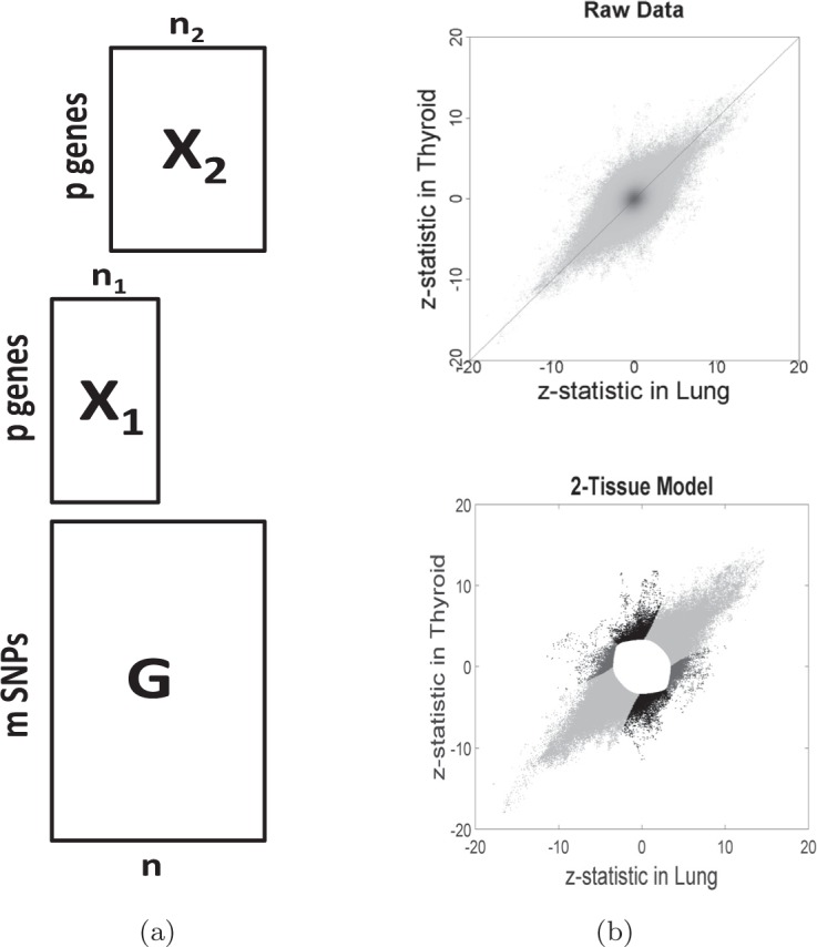
(a) Illustration of the typical data format with two tissues. Genotype data is available for SNPs and each of samples. Expression measurements are available for genes; sample sets for different tissues may not be the same. (b) z-statistics for lung and thyroid: density plot for all local gene–SNP pairs (top), and scatter plot for significant local gene–SNP pairs with tissue specificity by gray scale (bottom). The gene–SNP pairs deemed insignificant are omitted, leading to the white space at the center of the plot. The remaining points are colored according to their assessed tissue specificity: dark gray points correspond to the Lung-specific eQTL; black points correspond to the Thyroid-specific eQTL; light gray points correspond to the cross-tissue eQTL.

The contribution of the article is 5-fold: (i) introduction of a novel hierarchical Bayesian model for multi-tissue eQTL analysis; (ii) development of an efficient EM algorithm for estimating the parameters of the model; (iii) analysis of the properties of the model; (iv) rigorous theoretical arguments showing that model-based testing procedures control FDR under realistic assumptions; (v) applications to the GTEx data.

1.1. Related work

Most existing multi-tissue analyses extract eQTL individually from each tissue and then apply post hoc procedures to assess commonality and specificity (Dimas and others, 2009; Fu and others, 2012; Nica and others, 2011; Brown and others, 2013). Recently, several joint analysis approaches were proposed. Gerrits and others (2009) used an ANOVA model to study the genotype effect on a transcript across several cell types. Petretto and others (2010) used a sparse Bayesian multivariate regression model to identify eQTL at multiple loci for same transcripts in many tissues. More recently, Flutre and others (2013) developed a Bayesian model and a permutation-based approach to identify eQTL in multiple tissues. The computation is prohibitive for a moderate number of tissues and a large number of gene–SNP pairs. Sul and others (2013) proposed a “Meta-Tissue” method that combines linear mixed models with meta-analysis. It focuses on one gene–SNP pair at a time. However, the method cannot borrow strength across gene–SNP pairs for eQTL detection, or provide global parameter estimates to characterize eQTL patterns.

In the literature, eQTL analyses are generally divided into two categories: gene-level analysis and SNP-level analysis. The former focuses on the identification of eQTL genes, typically by averaging evidence over all candidate SNPs. The latter treats all gene–SNP pairs equally and aims at identifying significantly associated pairs. Both Gerrits and others (2009) and Sul and others (2013) studied eQTL at the SNP level while Petretto and others (2010) and Flutre and others (2013) are gene-level studies. Gene-level analysis tries to address linkage disequilibrium by assuming there is at most one causal SNP for each gene. However, it cannot provide a list of candidate SNP loci which are potential eQTL for a gene. In this article, we shall focus on the SNP level study, providing a complementary view of the problem. We will also address the computational issue and the lack-of-power concern by exploiting an empirical Bayes approach.

2. The MT-eQTL model

2.1. Format of multi-tissue eQTL data

The general data format for the multi-tissue eQTL problem is as follows. For each of donors we have full genotype information, and measurements of gene expression in at least one of tissues. Let be an matrix containing the measured genotype of each donor in the study at SNPs. The entries take values , , and , typically coded as the number of minor allele variants. Each column of corresponds to a donor, and each row corresponds to a SNP. The measured transcript levels for tissue are contained in a matrix , where is the number of genes, and is the number of donors for tissue . The number of donors can vary widely among tissues, and even if two tissues have similar numbers of samples, they may have few common donors. The data available for the purposes of multi-tissue eQTL analysis has the form . Figure 1a gives an illustration of the typical data format with two tissues.

In most cases, eQTL analysis is preceded by several preprocessing steps and covariate adjustment. Covariate adjustment is necessary because genotype and expression data usually contain confounding factors. Some confounders, such as gender, are observed, while others are of unknown technical or biological origin. To identify the unknown confounding factors, most studies use principal components, surrogate variables (Leek and Storey, 2007), or PEER factors (Stegle and others, 2012) as covariates. In Section 4.1, we shall discuss the preprocessing procedure of the GTEx data. For now, we just assume that the expression data and genotype data have been appropriately residualized for confounders, so the comparison of these residualized quantities are partial correlations adjusted for covariates.

2.2. Multivariate z-statistic from single tissue correlations

Denote a gene by and a SNP by . We focus on a subset of the full index set that consists of pairs such that SNP is located within a fixed distance (usually 100 Kilobases or 1 Megabase) of the transcription start site of gene .

Let be a gene-SNP pair of interest. Let and denote, respectively, the sample and population correlation of transcript and SNP in tissue . We use the Pearson product-moment correlation for several reasons: (i) with proper transformation of transcript data, the sample correlation has a known, normal distribution (Winterbottom, 1979), which is the basis of the proposed multi-tissue model; (ii) the Pearson correlation has close connection with the regression coefficient in a simple linear model relating transcript abundance and genotype (the foundation of most single-tissue eQTL studies). Note that the sample correlation depends only on the measurements from donors of tissue . The vector of correlations captures the association between the expression of transcript and the value of genotype in tissues. Relationships between different tissues will be reflected in correlations between the entries of . These features make a natural starting point for a multi-tissue eQTL model.

We build a multivariate model for the correlation vector . Let be the vector obtained by applying the Fisher transformation to each component of . Let be a scaling vector, where is the degrees of freedom for and , equal to minus the number of covariates used to correct genotype and expression for samples in tissue . Finally, define the vector where denotes the Hadamard (entry-wise) product of vectors and . Let denote the random vector for . If we assume that the expression measurements are approximately normal, standard arguments for the Fisher transformation (Winterbottom, 1979) imply that is approximately normal with mean and variance . By a routine multivariate extension of this fact, is approximately normally distributed with mean The variance stabilizing property of the Fisher transformation and our choice of scaling ensures that the variance of each entry of is close to one, regardless of . In particular, if the true correlation between transcript and SNP for tissue is zero, then is approximately standard normal. Thus the -th entry of the observed vector is a z-statistic for testing versus .

The use of z-statistics greatly reduces the data complexity and magnitude, without losing much information regarding gene-SNP associations. It facilitates statistical modeling and computation. Importantly, the components of are not independent due to the correlation of effect sizes and sample overlaps in different tissues. Capturing this dependence is one of the key features of the MT-eQTL model, which is described in detail below.

2.3. Hierarchical model

Let be a gene–SNP pair in . MT-eQTL is a multivariate, hierarchical Bayesian model for the random vector . In detail, we assume that

(2.1)

(2.2)

(2.3)

(2.4)

We briefly explain the rationale behind the model setup. The first relation is a consequence of the Fisher transformation, where denotes the true effect sizes of the gene–SNP pair across the tissues. The covariance matrix has diagonal values 1; its off-diagonal values capture the correlations between any two tissues arising from the underlying sampling process. In practice, the off-diagonal values are typically weakly positive due to overlapping donors for different tissues. Since the true effect sizes are unknown in practice, in (2.2), we build a hierarchical Bayesian model for based on two assumptions: when the SNP has no effect on the gene in a tissue, the true effect size is 0; when the SNP regulates the gene in a tissue, the true effect size follows a random distribution. Thus is represented as a Hadamard product of two random vectors, and .

The random vector is a configuration vector for the gene–SNP pair , indicating whether there is an eQTL in each of the K tissues. As in (2.3), the prior distribution of is a multinomial distribution with being the probability mass function. The multinomial distribution has components, each being a length- vector of and . In particular, indicates there is no eQTL in any tissue for the gene–SNP pair , and indicates there are eQTL in all tissues for this particular gene–SNP pair. The random vector is an eQTL effect size vector for the gene–SNP pair , capturing the true effect size in each tissue if there is an eQTL. In (2.4), we give a Gaussian prior, with mean and covariance . The mean parameter is a length- vector capturing the average eQTL effect sizes in all tissues, and the matrix represents the covariance structure of eQTL effect sizes across multiple tissues. The diagonal values indicate the variation of effect sizes in different tissues; and the off-diagonal values, typically strongly positive, reflect the relations of effect sizes between tissues.

In the model, there are four major parameters, , , and . The parameters characterize multi-tissue effect sizes for all gene–SNP pairs, and carry important biological interpretations. We will exploit an empirical Bayes approach to estimate all parameters from data.

2.4. Mixture model and estimation

The hierarchical model (2.1)–(2.4) describing the distribution of is fully specified by , which consists of real-valued parameters. Estimation of, and inference from, the hierarchical model is based on an equivalent mixture representation.

If is distributed as and is a fixed vector in , then one may readily verify that the entrywise product is distributed as . A straightforward argument then shows that the hierarchical model (2.1)–(2.4) is equivalent to a mixture model

(2.5)

The mixture model is readily interpretable. Each component of the model corresponds to a unique configuration , or equivalently, a unique pattern of tissue specificity. The model component corresponding to represents the case in which there are no eQTL in any tissue, and has associated (null) distribution . The model component corresponding to represents the case in which there are eQTL in every tissue, and has associated distribution . Other values of represent intermediate cases in which there are eQTL in some tissues (those with ) and not in others (those with ).

We adopt an empirical Bayes approach, estimating the model parameters from the observed z-statistics by maximizing the likelihood derived from (2.5). Beginning with the work of Newton and others (2001) and Efron and others (2001), empirical Bayes approaches have been applied to hierarchical models in a number of genetic applications, most notably the study of differential expression and co-expression in gene expression microarrays (Newton and others, 2004; Smyth and others, 2004; Efron, 2008; Dawson and Kendziorski, 2012).

Directly maximizing the joint log likelihood of the model (2.5) across gene–SNP pairs is computationally intractable. On the one hand, observations for different gene–SNP pairs may be correlated, as each gene may contain multiple SNPs and neighboring SNPs may have relatively strong linkage disequilibrium. On the other hand, the likelihood function for each gene–SNP pair has components, each corresponding to a weighted multivariate Gaussian likelihood function with overlapping model parameters. Note that the parameters in the model (2.5) determine, and are determined by, the marginal distribution of the vectors , and do not depend on their joint distribution. We address the issue of correlated observations by maximizing a marginal composite likelihood, which is defined as the product of the marginal likelihoods of all considered gene–SNP pairs. As such, it does not attempt to capture correlation between different gene–SNP pairs. For typical eQTL analyses, in which the number of gene–SNP pairs is large and average pairwise correlations are low, we expect the use of marginal composite likelihood estimation has little effect on statistical efficiency.

To address the difficulty of parameter estimation, we exploit an EM algorithm by treating the underlying configuration vector for each gene–SNP pair as a latent variable. As a result, the estimation of the probability mass function can be separated from the estimation of , and . The optimization with respect to has a closed-form solution in each iteration. Furthermore, in cis-eQTL analysis, the null configuration and the full alternative configuration together usually account for the majority of the prior weight. When estimating , and , if we only focus on the log likelihood terms corresponding to these two configurations, each parameter has an explicit estimate. As such, we use a modified EM algorithm with the two-term approximation, which greatly reduces the computational cost. Simulation studies show that such approximation has little affect on the accuracy of the estimation. More details of the model fitting algorithm can be found in Section 1 of Supplementary material available at Biostatistics online.

2.5. Marginal compatibility

In eQTL studies with multiple tissues, it is desirable if the model for a subset of tissues is compatible with the model for a superset of tissues in the sense that the former can be obtained from the latter via marginalization. We refer to this property as marginal compatibility. From the model interpretation point of view, the property guarantees that parameters (e.g. prior probabilities of different eQTL configurations, covariance of effect sizes in different tissues) corresponding to a set of tissues do not depend on whether we observe just those tissues or a superset of the tissues. It is crucial in multi-tissue eQTL studies as we essentially always analyze a set of some hypothetical superset of tissues that we do not observe. From the model fitting point of view, with the property, we only need to fit the full model with all available tissues once. The model for any subset of tissues can be obtained directly through marginalization without refitting.

To elaborate, let be a subset of tissues, with . The mixture model (2.5) has two important compatibility properties: (i) the marginalization of the full model to has the same general form as the model derived from alone; and (ii) the parameters of the marginal model are obtained by restricting the parameters of the full model to . The following definition and lemma makes these statements precise. See Section 2 of Supplementary material available at Biostatistics online for a proof of the lemma.

Definition: Let with cardinality . For each vector let be the vector obtained by restricting to the entries in . Similarly, for each matrix let be the matrix obtained by retaining only the rows and columns with indices in . Note that if is non-negative (positive) definite, then is non-negative (positive) definite as well.

Lemma 2.1

If be a random vector having the mixture distribution (2.5), then

where is the probability mass function on obtained by marginalizing to , i.e. .

3. Multi-tissue eQTL inference

Once fit, the mixture model (2.5) provides the basis for inference about eQTL across tissues. When the number of gene–SNP pairs is large, as in the GTEx example in Section 4, can be accurately estimated from data. At the level of posterior inference for gene–SNP pairs, we therefore regard as fixed and known. For data sets with small sample sizes, approximate standard errors for the components of can be obtained from the likelihood via the observed information matrix.

Denote the density of the distribution associated with the configuration by . Thus under the mixture model (2.5) the random vector has density , . In view of this expression and the hierarchical model (2.1)–(2.4), one may regard as one element of a jointly distributed pair , where

(3.1)

We carry out multi-tissue eQTL analysis based on the posterior distribution of the configuration given the observed vector of z-statistics . Two inference problems are of central interest: one is eQTL detection, in all tissues and in a subset of tissues; the other is the assessment of eQTL tissue specificity given eQTL is present in at least one tissue.

3.1. Detection of eQTL using the local false discovery rate

A primary goal of multi-tissue analysis is testing each transcript–SNP pair for the presence of an eQTL in at least one tissue. This can be formulated as a multiple testing problem:

(3.2)

For the null hypothesis asserts that SNP is not an eQTL for transcript in any tissue, while the alternative asserts that there is an eQTL between and in at least one tissue.

The null hypotheses can also be expressed in the form One may derive a p-value for each directly from the null distribution, and convert it to control the overall false discovery rate (FDR) (cf. Benjamini and Hochberg, 1995; Storey and Tibshirani, 2003). However, this procedure ignores relevant information about the distribution of under the alternative that is contained in the mixture model.

We address the multiple testing problem (3.2) using the local FDR introduced by Efron and others (2001) in the context of an empirical Bayes analysis of differential expression in microarrays. Other applications of the local FDR to genomic problems can be found in Newton and others (2004), Efron (2007), and Efron (2008). To simplify notation, let denote a generic pair distributed as .

Definition: The local FDR of an observed z-statistic vector under the model (2.5) is defined by

(3.3)

Let be a target FDR for the multiple testing problem (3.2). Vectors for which the local false discovery rate is small provide evidence for the alternative . We carry out testing of gene–SNP pairs using a step-up procedure applied to the running average of the ordered local false discover rates (Newton and others, 2004; Cai and Sun, 2009).

Local FDR Step-Up Procedure: Target FDR

• 1. Given: Observed -statistic vectors .

• 2. Enumerate the elements of as so that .

• 3. Reject hypotheses , where is the largest integer such that .

3.2. Theoretical justification of the local FDR approach

In order to better understand the local FDR step-up procedure, and to assess its performance, it is useful to express the procedure in an equivalent form. As noted by Efron and others (2001), the false discovery rate associated with a rejection region for the multiple testing problem (3.2) is given by . They establish the following elementary fact, which exhibits a connection between FDR and local FDR.

Proposition 3.1

If is such that , then .

As noted above, vectors for which is small provide evidence against , so it is natural to reject when falls below an appropriate threshold. Consider rejection regions of the form for . Given a target FDR , we wish to find such that . By Proposition 3.1 this is equivalent to finding such that , where

The empirical analog of is the ratio

which depends only on and the observed vectors . The function is strictly increasing and continuous (see Section 3.1 of Supplementary material available at Biostatistics online for proof). Thus if and were equal, the local FDR step-up procedure and the idealized threshold procedure would coincide. In general, and will be different, but multiplying the numerator and denominator of by it is evident that the two functions will be close if is large and the dependence among the observed -vectors is not extreme. Asymptotic control of the FDR by the step-up procedure is established in Theorem 3.2 below. The proof can be found in Section 3 of Supplementary material available at Biostatistics online.

Let be an infinite index set, and let be a sequence of finite subsets of . Let be a target FDR that is less than the maximum value of . For each let be jointly distributed pairs having the same distribution as . We wish to assess the performance of the local FDR step-up procedure, which rejects when where

The number of false discoveries and total discoveries for the procedure are equal to

Theorem 3.2

Let have joint distribution given by Model (3.1) with parameters . Assume that is positive definite and that the diagonal entries of are positive. If in probability for each then as .

The ratio of expectations is sometimes referred to as the marginal false discovery rate (m-FDR). Cai and Sun (2009) established optimality properties and m-FDR control of several local FDR based testing procedures, including the step-up procedure used here, under independence and monotonicity assumptions. However, these assumptions are typically violated in the setting of interest to us here. The monotonicity assumption, which in the present case involves the relationship between the distributions of the local FDR under and , does not appear to hold. Moreover, in eQTL data there are typically significant correlations between nearby SNPs (linkage disequilibrium), leading to to complex, non-stationary correlations between the gene-SNP based vectors .

Theorem 3.2 makes no explicit assumptions on the joint distribution of the vectors ; instead it relies on the relatively weak condition that in probability. This condition holds, for example, under the (very mild) assumption that the variance of the numerator and the denominator of are of order . The variance decay assumption concerns the family of all gene–SNP pairs, across all measured genes instead of a single gene. Although the SNPs co-located with a particular gene may be highly correlated, correlations are generally weak, or zero, across distant genes. These distal pairs dominate the index set , and so the variance decay assumption should be satisfied in any cis-eQTL analysis involving a large number of genes. When the assumption holds, the conclusion of the theorem may be strengthened to .

3.3. Analysis for subsets of tissues

In some problems, a subset of the available tissues may be of primary interest. The multiple testing framework described above can be adapted to the tissues in in two primary ways. The first is to construct a model based only on the tissues in and use the resulting local FDR to identify multi-tissue eQTL. However, this approach does not make use of the available data from tissues outside and as such it does not borrow strength from commonalities among tissues. As an alternative, one may use the marginal local FDR for , defined by

(3.4)

Here and denote, respectively, the restriction of the vectors and to the tissues in , while , and correspond to the full model (2.5). We emphasize that the marginal local FDR is a function of the complete vector of z-statistics, and therefore depends on the fitted model for the full set of tissues. In Section 4.3, we have shown that the marginal local FDR derived from the full data set is uniformly more powerful than the local FDR derived from a subset of the data in detecting eQTLs in a subset of tissues. More numerical results can be found in Section 4.3 of Supplementary material available at Biostatistics online.

3.4. Assessments of tissue specificity

Testing gene–SNP pairs is typically the first step in multi-tissue eQTL analysis. Rejection of is based on evidence that is an eQTL in at least one of the available tissues. More detailed statements about the pattern of eQTL across tissues can be made using information about the full configuration vector . If the hypothesis is rejected, a natural estimate of is the maximum a posteriori (MAP) configuration defined by

As an alternative, one may compute the marginal posterior probability of an eQTL in each tissue , namely and declare an eQTL in tissue if this marginal probability exceeds a predefined threshold. Both MAP and thresholding of the marginal posterior extend to subsets of tissues.

3.5. Testing a family of configurations

The goal of the multiple testing problem (3.2) is to determine whether the configuration of a gene–SNP pair is equal to or belongs to the complementary set . More generally, one may test membership of in any fixed subset of configurations. The associated testing problem can be written as

(3.5)

A test statistic for (3.5) can be obtained by marginalizing the full local FDR (3.3) as

The local FDR step-up procedure can then be applied to the values in order to control the overall FDR in (3.5).

4. GTEx data analysis

In this section, we apply the MT-eQTL model and inference procedures to the GTEx pilot data freeze (The GTEx Consortium, 2015). A pointer to the publicly available data is at http://www.broadinstitute.org/gtex/.

4.1. Data preprocessing

We focus on nine primary tissues having between 80 and 160 samples: adipose, artery, blood, heart, lung, muscle, nerve, skin, and thyroid. In what follows, tissues will be ordered alphabetically. In total, there are 175 genotyped individuals with expression data in at least one of these tissues (the sample information can be found in Figure S1 of Supplementary material available at Biostatistics online).

Each entry of the genotype data matrix records the number of minor allele variants of one donor at one SNP locus. Any missing value at a locus was imputed by the corresponding row average. Loci with minor allele frequency less than 5% in all genotyped individuals were discarded, resulting in slightly less than 7 million SNPs. The expression level for each gene in each tissue and sample is measured by the number of mapped reads per kilobase per million reads (RPKM). Genes having fewer than samples with RPKM greater than in some tissue were discarded, leaving slightly more than 20,000 genes. To improve robustness, the gene expression values across samples in a tissue were inverse quantile normalized.

Fifteen PEER factors were identified from the expression data from each tissue, and three principal components were identified from the genotype data. With an additional covariate for gender, we obtained nineteen covariates in total. For each tissue, the confounding effects were adjusted by residualizing the expression data and the corresponding genotype data on nineteen covariates respectively. Consequently, the degree of freedom for each tissue is equal to the sample size in that tissue minus 19.

4.2. Model fit

We focus on testing of cis-eQTL, restricting our attention to SNPs that lie within 100 kilobases of the transcription start site of a gene, yielding roughly 10 million gene–SNP pairs of interest. Subsequently, the full 9D MT-eQTL model was fit using the modified EM algorithm described in Section 2.4 with the parameter set to zero. Fitting the full model took less than 24 hours, and required less than 8 gigabytes of RAM, on a desktop computer with 2.93GHz Intel Xeon CPU. A comparison of timing results for fitting sub-models of different dimensions between our method and the Meta-Tissue method (Sul and others, 2013) can be found in Section 5 of Supplementary material available at Biostatistics online.

In what follows we denote the estimated model parameters by . Values of the estimated parameters can be found in Section 5 of Supplementary material available at Biostatistics online. The off-diagonal values of are all positive but small in scale (between and ), suggesting that donor overlap among tissues and other features of the experimental design have a weak but positive effect on the correlations of effect sizes across tissues. The diagonal values of indicate modest heterogeneity of effect size variation across tissues. The off-diagonal values of reflect positive, often large, correlation of effect sizes arising from commonalities among tissues.

The fitted probability mass function assigns probabilities to each of the possible eQTL configurations. The most likely configuration is with , indicating that about 68% of the gene–SNP pairs do not have an eQTL in any tissue. This is consistent with previous studies (Wright and others, 2014). To summarize , we sum up the prior probabilities of configurations with the same Hamming weight (defined as the number of 1s in a length-9 binary configuration sequence). This provides an overview of the overall probability of seeing an cis-eQTL in k tissues, where ranges from to . We note, however, that the probabilities for configurations with the same Hamming weight may be quite different. The total prior probabilities are shown in Figure 2 in the log scale. The U-shape curve indicates that for cis-eQTL analysis, the most likely configurations are eQTL in no tissue, in a single tissue, or in all tissues, and the least likely configurations are those with eQTL in roughly half the tissues. We remark that the pattern may only apply to cis-eQTL but not to trans-eQTL.

Fig. 2.

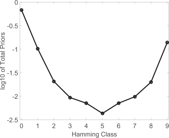
Summary of the estimated eQTL probabilities from the cis-eQTL analysis of the GTEx data. Each circle represents the log (base 10) of the probability of a gene–SNP pair having eQTL in out of 9 tissues, where ranges from to .

4.3. Results

Applied to the full 9D model with FDR threshold , the local FDR step-up procedure identified roughly 1.28 million gene–SNP pairs (roughly 12% of the total) with an eQTL in at least one tissue. We subsequently applied the MAP rule to each significant discovery in order to assess tissue specificity. To validate the discoveries, we also applied the Meta-Tissue method to the same data set. Meta-Tissue produces a p value for each gene–SNP pair for testing the existence of eQTL in any tissue. We further adjusted the p values (Benjamini and Yekutieli, 2001) to control the FDR. About 80% of the MT-eQTL discoveries (i.e. 1.03 million) are replicated in Meta-Tissue, providing a highly concordant result. We further investigated the unique discoveries of each method (about 250 thousand from MT-eQTL, and 177 thousand from Meta-Tissue). The left panel of Figure 3 shows the Meta-Tissue p values of the unique discoveries from MT-eQTL. Small p values are enriched, indicating the unique MT-eQTL discoveries are well supported by Meta-Tissue. The right panel of Figure 3 presents the MT-eQTL local FDRs of the unique discoveries from Meta-Tissue. The unique Meta-Tissue discoveries are only moderately supported by MT-eQTL. The MT-eQTL provides a systematic way to leverage information across gene–SNP pairs, and offers explicit estimates of model parameters with critical biological interpretation.

Fig. 3.

The left panel is the histogram of the Meta-Tissue p values for the 250 thousand unique discoveries from MT-eQTL, from the GTEx analysis of eQTL in at least one tissue; the right panel is the histogram of the MT-eQTL local FDRs for the 177 thousand unique discoveries in Meta-Tissue.

A unique advantage of MT-eQTL over Meta-Tissue is the ease of eQTL tissue specificity assessment. To facilitate the visualization of eQTL discoveries, let us focus on a two-tissue MT-eQTL model. As an example, Figure 1b shows scatter plots of z-statistics for lung and thyroid. The upper panel shows the density plot of the raw z-statistics (MT-eQTL input); the lower panel only shows the discoveries with eQTL in at least one of the tissues (MT-eQTL output). The z-statistic vectors deemed insignificant are omitted, leading to the white space at the center of the plot. The remaining points are colored according to their assessed tissue specificity based on the MAP approach: dark gray represents the configuration in which there is an eQTL in tissue 1 but not tissue 2; black represents the configuration in which there is an eQTL in tissue 2 but not tissue 1; and light gray represents the configuration in which there is an eQTL in both tissues. The overall shape of each plot is a tilted ellipse, with extreme values along the main diagonal and, to a lesser extent, along the coordinate axes. As expected, significant points close to one of the coordinate axes show evidence for an eQTL in a single tissue (tissue specific eQTL), while those along the positive diagonal show evidence for eQTL in both tissues (common eQTL). We remark that this analysis easily extends to an arbitrary number of tissues.

MT-eQTL also effectively leverages information in multiple tissues to improve eQTL detection in a single or a subset of tissues. To investigate how the use of auxiliary tissues increases statistical power, we studied a sequence of nested MT-eQTL models and focused on eQTL discoveries in a single tissue. For each of the nine tissues, we first fitted the 1-dimensional model with just the primary tissue and then added other tissues one by one alphabetically to get a sequence of super-models. For each considered model, we applied the adaptive thresholding procedure to the marginal local FDR for the primary tissue, and recorded the number of significant discoveries in that tissue. Figure 4 shows the number of significant discoveries versus the dimension of a model. Each curve corresponds to a case where one of the nine tissues is set to be the primary tissue. The number of eQTL discoveries in each primary tissue increases with the dimension of a model.

Fig. 4.

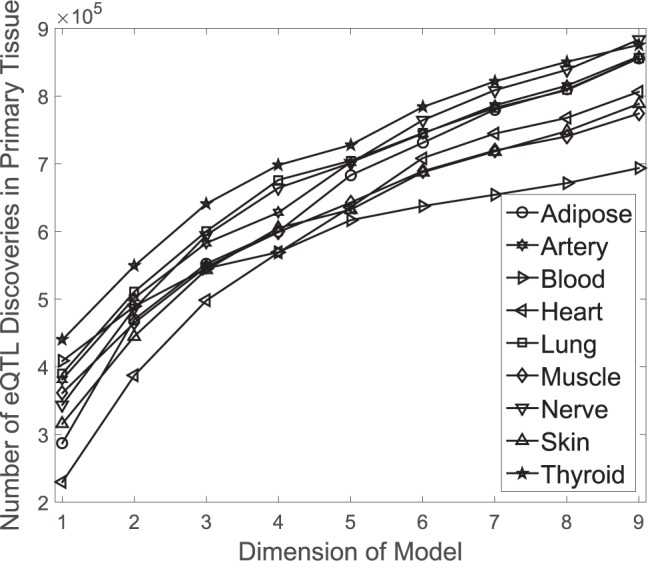
The number of significant discoveries in a primary tissue versus the dimension of a MT-eQTL model. Each curve corresponds to a case where one of the nine tissues is set to be the primary tissue. The FDR threshold is fixed to be .

5. Conclusion

In this article, we proposed a hierarchical Bayesian model, MT-eQTL, for multi-tissue eQTL analysis. We adopted an empirical Bayes approach to estimate the model and to perform inferences. We also proved a substantial theoretical property to support the method in a realistic setting. The proposed methodology greatly enhances classical single-tissue eQTL analysis methods by accounting for the information shared among tissues.

There are a number of interesting directions for future research. Perhaps the most important is to extend the proposed framework to a large number (e.g. ) of tissues. The large tissue setting poses real challenges as the total number of configurations grows exponentially in the number of tissues, making the current implementation excessively slow and computationally costly. Another direction is to relax the assumption that the covariance matrix in Model (2.5) is constant across gene–SNP pairs. Different genes may have distinct correlation patterns between tissues, which might warrant the use of gene-specific covariance matrices in setting where the number of samples is large. Lastly, it is of interest to extend the method to the identification of trans-eQTLs, which exhibit higher levels of tissue-specificity than (Jo and others, 2016).

Supplementary material

Supplementary material is available at http://biostatistics.oxfordjournals.org.

Funding

National Institute of Health (NIH) (Grant R01 MH090936 and MH101819-0); National Science Foundation (NSF) (Grant DMS 0907177 and DMS 1310002); and Environmental Protection Agency (EPA) (Grant STAR RD83580201), in part.

References

- Benjamini Y. and Hochberg Y. (1995). Controlling the false discovery rate: a practical and powerful approach to multiple testing. Journal of the Royal Statistical Society. Series B (Methodological) 57, 289–300. [Google Scholar]
- Benjamini Y. and Yekutieli D. (2001). The control of the false discovery rate in multiple testing under dependency. Annals of Statistics 29, 1165–1188. [Google Scholar]
- Brown C. D., Mangravite L. M. and Engelhardt B. E. (2013). Integrative modeling of eQTLs and cis-regulatory elements suggests mechanisms underlying cell type specificity of eQTLs. PLoS Genetics 9, e1003649. [DOI] [PMC free article] [PubMed] [Google Scholar]
- Cai T. T. and Sun W. (2009). Simultaneous testing of grouped hypotheses: finding needles in multiple haystacks. Journal of the American Statistical Association 104, 1467–1481. [Google Scholar]
- Dawson J. A. and Kendziorski C. (2012). An empirical Bayesian approach for identifying differential coexpression in high-throughput experiments. Biometrics 68, 455–465. [DOI] [PMC free article] [PubMed] [Google Scholar]
- Dimas A. S., Deutsch S., Stranger B. E., Montgomery S. B., Borel C., Attar-Cohen H., Ingle C., Beazley C., Gutierrez Arcelus M., Sekowska M.. and others (2009). Common regulatory variation impacts gene expression in a cell type–dependent manner. Science 325, 1246–1250. [DOI] [PMC free article] [PubMed] [Google Scholar]
- Efron B. (2007). Size, power and false discovery rates. The Annals of Statistics 35, 1351–1377. [Google Scholar]
- Efron B. (2008). Microarrays, empirical Bayes and the two-groups model. Statistical Science, 1–22. [Google Scholar]
- Efron B., Tibshirani R., Storey J. D. and Tusher V. (2001). Empirical Bayes analysis of a microarray experiment. Journal of the American Statistical Association 96, 1151–1160. [Google Scholar]
- Flutre T., Wen X., Pritchard J. and Stephens M. (2013). A statistical framework for joint eQTL analysis in multiple tissues. PLoS Genetics 9, e1003486. [DOI] [PMC free article] [PubMed] [Google Scholar]
- Fu J., Wolfs M. G., Deelen P., Westra H. J., Fehrmann R. S., Te Meerman G. J., Buurman W. A., Rensen S. S., Groen H. J., Weersma R. K.. and others (2012). Unraveling the regulatory mechanisms underlying tissue-dependent genetic variation of gene expression. PLoS Genetics 8, e1002431. [DOI] [PMC free article] [PubMed] [Google Scholar]
- Gerrits A., Li Y., Tesson B. M., Bystrykh L. V., Weersing E., Ausema A., Dontje B., Wang X., Breitling R., Jansen R. C. and de Haan G. (2009). Expression quantitative trait loci are highly sensitive to cellular differentiation state. PLoS Genetics 5, e1000692. [DOI] [PMC free article] [PubMed] [Google Scholar]
- Jo B., He Y., Strober B. J., Parsana P., Aguet F., Brown A. A., Castel S. E., Gamazon E. R., Gewirtz A., Gliner G.. and others (2016). Distant regulatory effects of genetic variation in multiple human tissues. bioRxiv, 074419. [Google Scholar]
- Kendziorski C. and Wang P. (2006). A review of statistical methods for expression quantitative trait loci mapping. Mammalian Genome 17, 509–517. [DOI] [PubMed] [Google Scholar]
- Leek J. T. and Storey J. D. (2007). Capturing heterogeneity in gene expression studies by surrogate variable analysis. PLoS Genetics 3, e161. [DOI] [PMC free article] [PubMed] [Google Scholar]
- Newton M. A., Kendziorski C. M., Richmond C. S., Blattner F. R. and Tsui K.-W. (2001). On differential variability of expression ratios: improving statistical inference about gene expression changes from microarray data. Journal of Computational Biology 8, 37–52. [DOI] [PubMed] [Google Scholar]
- Newton M. A., Noueiry A., Sarkar D. and Ahlquist P. (2004). Detecting differential gene expression with a semiparametric hierarchical mixture method. Biostatistics 5, 155–176. [DOI] [PubMed] [Google Scholar]
- Nica A. C., Parts L., Glass D., Nisbet J., Barrett A., Sekowska M., Travers M., Potter S., Grundberg E., Small K.. and others (2011). The architecture of gene regulatory variation across multiple human tissues: the MuTHER study. PLoS Genetics 7, e1002003. [DOI] [PMC free article] [PubMed] [Google Scholar]
- Petretto E., Bottolo L., Langley S. R., Heinig M., McDermott-Roe C., Sarwar R., Pravenec M., Hübner N., Aitman T. J., Cook S. A. and Richardson S. (2010). New insights into the genetic control of gene expression using a Bayesian multi-tissue approach. PLoS Computational Biology 6, e1000737. [DOI] [PMC free article] [PubMed] [Google Scholar]
- Smyth G. K. (2004). Linear models and empirical Bayes methods for assessing differential expression in microarray experiments. Statistical Applications in Genetics and Molecular Biology 3, 3. [DOI] [PubMed] [Google Scholar]
- Stegle O., Parts L., Piipari M., Winn J. and Durbin R. (2012). Using probabilistic estimation of expression residuals (peer) to obtain increased power and interpretability of gene expression analyses. Nature Protocols 7, 500–507. [DOI] [PMC free article] [PubMed] [Google Scholar]
- Storey J. D. and Tibshirani R. (2003). Statistical significance for genomewide studies. Proceedings of the National Academy of Sciences 100, 9440–9445. [DOI] [PMC free article] [PubMed] [Google Scholar]
- Sul J. H., Han B., Ye C., Choi T. and Eskin E. (2013). Effectively identifying eQTLs from multiple tissues by combining mixed model and meta-analytic approaches. PLoS Genetics 9, e1003491. [DOI] [PMC free article] [PubMed] [Google Scholar]
- The GTEx Consortium. (2015). The genotype-tissue expression (gtex) pilot analysis: multitissue gene regulation in humans. Science 348, 648–660. [DOI] [PMC free article] [PubMed] [Google Scholar]
- Winterbottom A. (1979). A note on the derivation of fisher’s transformation of the correlation coefficient. The American Statistician 33, 142–143. [Google Scholar]
- Wright F. A., Shabalin A. A. and Rusyn I. (2012). Computational tools for discovery and interpretation of expression quantitative trait loci. Pharmacogenomics 13, 343–352. [DOI] [PMC free article] [PubMed] [Google Scholar]
- Wright F. A., Sullivan P. F., Brooks A. I., Zou F., Sun W., Xia K., Madar V., Jansen R., Chung W., Zhou Y. H.. and others (2014). Heritability and genomics of gene expression in peripheral blood. Nature Genetics 46, 430–437. [DOI] [PMC free article] [PubMed] [Google Scholar]
Associated Data
This section collects any data citations, data availability statements, or supplementary materials included in this article.