Abstract
Background
Dynamic modelling is a core element in the systems biology approach to understanding complex biosystems. Here, we consider the problem of parameter estimation in models of biological oscillators described by deterministic nonlinear differential equations. These problems can be extremely challenging due to several common pitfalls: (i) a lack of prior knowledge about parameters (i.e. massive search spaces), (ii) convergence to local optima (due to multimodality of the cost function), (iii) overfitting (fitting the noise instead of the signal) and (iv) a lack of identifiability. As a consequence, the use of standard estimation methods (such as gradient-based local ones) will often result in wrong solutions. Overfitting can be particularly problematic, since it produces very good calibrations, giving the impression of an excellent result. However, overfitted models exhibit poor predictive power.
Here, we present a novel automated approach to overcome these pitfalls. Its workflow makes use of two sequential optimisation steps incorporating three key algorithms: (1) sampling strategies to systematically tighten the parameter bounds reducing the search space, (2) efficient global optimisation to avoid convergence to local solutions, (3) an advanced regularisation technique to fight overfitting. In addition, this workflow incorporates tests for structural and practical identifiability.
Results
We successfully evaluate this novel approach considering four difficult case studies regarding the calibration of well-known biological oscillators (Goodwin, FitzHugh–Nagumo, Repressilator and a metabolic oscillator). In contrast, we show how local gradient-based approaches, even if used in multi-start fashion, are unable to avoid the above-mentioned pitfalls.
Conclusions
Our approach results in more efficient estimations (thanks to the bounding strategy) which are able to escape convergence to local optima (thanks to the global optimisation approach). Further, the use of regularisation allows us to avoid overfitting, resulting in more generalisable calibrated models (i.e. models with greater predictive power).
Electronic supplementary material
The online version of this article (10.1186/s12859-019-2630-y) contains supplementary material, which is available to authorized users.
Keywords: Parameter estimation, Global optimisation, Regularisation, Parameter bounding, Dynamic modelling
Background
Oscillations and sustained rhythms are pervasive in biological systems and have been deeply studied in areas such as metabolism [1–5], the cell cycle [6–9], and Circadian rhythms [10–16], to name but a few. In recent years, many research efforts have been devoted to the development of synthetic oscillators [17–20], including tunable ones [21–24].
Mathematical and computational approaches have been widely used to explore and analyse these complex dynamics [25–32]. Model-based approaches have also allowed for the identification of design principles underlying circadian clocks [12, 33] and different types of biochemical [34] and genetic oscillators [35–39]. Similarly, the study of the behaviour of populations of coupled oscillators has also greatly benefited from mathematical analysis and computer simulations [40–47].
A number of approaches can be used to build mathematical models of these biological oscillators [48–52]. This process is sometimes called reverse engineering, inverse problem solving or dynamic model identification [53–55]. Model calibration (i.e. parameter estimation or data fitting) is a particularly important and challenging sub-problem in the identification process [56–64]. Different strategies have been specially developed and applied to calibrate models of oscillators [32, 50, 65–71] and to characterise and explore their parameter space [31, 72–76].
In this study, we consider parameter estimation in mechanistic dynamic models of biological oscillators. From all the issues that plague model calibration [77], we pay special attention to three that are particularly problematic in oscillatory models: huge search spaces, multimodality and overfitting. We also discuss how to handle lack of identifiability.
Methods
Models of biological oscillators
Here, we consider mechanistic models of oscillatory biological systems given by deterministic nonlinear ordinary differential (ODEs). The general model structure is:
| 1 |
| 2 |
| 3 |
where represents the states of the system as time-dependent variables, under the initial conditions x0, is the parameter vector, u(t) represents any time-dependent input (e.g. stimuli) affecting the system and is the time variable. ΨO represents the set of all possible oscillatory dynamics. The observation function maps the states to a vector of observables , i.e. the state variables that can be measured. While the methodology here is developed for and tested on oscillatory models, it is not strictly restricted to models that exhibit such behaviour.
Formulation of the parameter estimation problem
We now consider the parameter estimation problem considering dynamic models described by the above Eqs. (1 – 3). We formulate this estimation problem as a maximisation of the likelihood function given by:
| 4 |
where Ne is the number of experiments, Ny,k the number of observables in those experiments, Nt,k,j is the number of time points for each observable, represents the measured value for the ith time point of the jth observable in the kth experiment, and σkji represents its corresponding standard deviation. Under specific conditions [78], the maximisation of the likelihood formulation is equivalent to the minimisation of the weighted least squares cost given by:
| 5 |
Using the above cost, the estimation problem can be formulated as the following minimisation problem:
| 6 |
subject to the dynamic system described by Eqs. (1–3), and also subject to the parameter bounds:
| 7 |
We denote the solution to this minimisation problem as . In principle, this problem could be solved by standard local optimisation methods such as Gauss-Newton or Levenberg-Marquardt. However, as described next, there are many pitfalls and issues that complicate the application of these methods to many real problems.
Pitfalls and perils in the parameter estimation problem
Numerical data fitting in nonlinear dynamic models is a hard problem with a long list of possible pitfalls, including [77]: a lack of identifiability, local solutions, badly scaled data and parameters, oscillating dynamics, inconsistent constraints, non-differentiable model functions, slow convergence and errors in experimental data. It should be noted that several of these difficulties are interrelated, e.g. a lack of practical identifiability can be due to noisy and non-informative data and will result in slow convergence and/or finding local solutions.
In the case of oscillators, the above issues apply, particularly multimodality and lack of identifiability. However, there are at least two additional important difficulties that must be also considered: overfitting (i.e. fitting the noise rather than the signal) and very large search spaces (which creates convergence difficulties and also makes it more likely the existence of additional local optima). Although these four issues are all sources of difficulties for proper parameter estimation, the last two have been less studied.
Lack of identifiability
The objective of identifiability analysis is to find out whether it is possible to uniquely estimate the values of the unknown model parameters [79]. It is useful to distinguish between two types of identifiability: structural and practical. Structural identifiability [80, 81] studies if the model parameters can be uniquely determined assuming ideal conditions for the measurements and therefore only considering the model dynamics and the input-output mapping (i.e. what is perturbed and what is observed). Structural identifiability is sometimes called a priori identifiability. Despite recent advances [82–84], structural identifiability analysis remains difficult to apply to large dynamic models with arbitrary nonlinearities.
It is important to note that, even if structural identifiability holds, unique determination of parameter values is not guaranteed since it is a necessary condition but not a sufficient one. Practical identifiability analysis [85–87] considers experimental limitations, i.e. it aims to find if parameter values can be determined with sufficient precision taking into account the limitations in the measurements (i.e. the amount and quality of information in the observed data). Practical (sometimes called a posteriori) identifiability analysis will typically compute confidence intervals of the parameter values. Importantly, it can also be taken into account as an objective in optimal experimental design [86].
Multimodality
Schittkowski [77] puts emphasis on the extremely difficult nature of data fitting problems when oscillatory dynamics are present: the cost function to be minimised will have a large number of local solutions and an irregular structure. If local optimisation methods are used, they will likely converge to one of these local solutions (typically the one with the basin of attraction that includes the initial guess). Several researchers have studied the landscape of the cost functions being minimised, describing them as very rugged and with multiple local minima [77, 88, 89]. Thus, this class of problems clearly needs to be solved with some sort of global optimisation scheme as illustrated in a number of studies during the last two decades [57, 86, 90–93].
The simplest global optimisation approach (and widely used in parameter estimation) is the so-called multi-start method, i.e. a (potentially large) number of repeated local searchers initialised from usually random initial points inside the feasible space of parameters. Although a number of studies have illustrated the power of this approach [94–96], others have found that it can be inefficient [92, 97–99]. This is especially the case when there is a large number of local solutions: in such situations, the same local optima will be repeatedly found by many local searches, degrading efficiency.
Thus, several methods have tried to improve the performance of the plain multi-start method by incorporating mechanisms to avoid repeated convergence to already found local solutions. This is the case of hybrid metaheuristics, where a global search phase is performed via diversification mechanisms and combined with local searches (intensification mechanisms). In this context, the enhanced scatter search (eSS) method has shown excellent performance [64, 97, 99, 100]. Here we will use an extension of the eSS method distributed in the MEIGO toolbox [101] as the central element of our automated multi-step approach. We have modified the MEIGO implementation of eSS in several ways, as detailed in Additional file 1. In order to illustrate the performance and robustness of eSS with respect to several state-of-the-art local and global solvers, we provide a critical comparison in Additional file 2.
Huge search spaces
In this study, we consider the common case scenario where little prior information about (some or all of the) parameters is available and therefore we need to consider ample bounds in the parameter estimation. These huge parameter bounds complicate convergence from arbitrary initial points, increase computation time and make it more likely that we will have a large number of local solutions in the search space. Although deterministic methods, which could be used to systematically reduce these bounds exist [102–104], currently they do not scale up well with problem size. Such techniques therefore can not be applied to problems of realistic size. Some analytical approaches have also been used for the analysis of biological oscillators [26, 31]. Alternatively, non-deterministic sampling techniques have been used to explore the parameter space and identify promising regions consistent with pre-specified dynamics [105]. Inspired by these results, we will re-use the sampling performed during an initial optimisation phase to reduce the parameter bounds.
Overfitting
Overfitting describes the problem associated with fitting the noise in the data, rather than the signal. Overfitted models can be misleading as they present a low-cost function value, giving the false impression that they are well-calibrated models that can be useful for making predictions. However, overfitted models have poor predictive power, i.e. they do not generalise well and can result in major prediction artefacts [106]. In order to fight overfitting, a number of regularisation techniques have been presented. Regularisation methods originated in the area of inverse problem theory [107]. Most regularisation schemes are based on adding a penalty term to the cost function, based on some prior knowledge of the parameters. This penalty makes the problem more regular, in the sense of reducing ill-conditioning and by penalising wild behaviour. Regularisation also can be used to minimise model complexity.
However, regularisation methods for nonlinear dynamics models remain an open question [99]. Further, these methods require some prior knowledge about the parameters and a tuning process which can be cumbersome and computationally demanding. Here, we will present a workflow that aims to automate this process.
Small illustrative example
In order to graphically illustrate several of the above issues, let us consider the ENSO problem, a small yet challenging example taken from the National Institute of Standards (NIST) nonlinear least squares (NLLS) test suite [108].
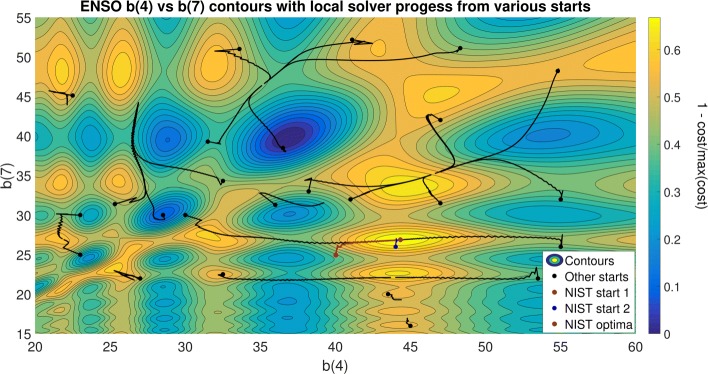
To visualise the multimodality of this problem, we can use contour plots of the cost function for pairs of parameters, as shown in Fig. 1. In this figure we also show the convergence paths followed by a multi-start of a local optimisation method (NL2SOL [109]), illustrating how most of the runs converge to local solutions or saddle points close to the initial point. We can also see how different runs converge to the same local solutions, explaining the low efficiency of multi-start for problems with many local optima. We also provide additional figures for this problem in Additional file 1.
Fig. 1.
ENSO problem NL2SOL contours: contours of the cost function (nonlinear least squares) for parameters b4 and b7, and trajectories of a multi-start of the NL2SOL local solver
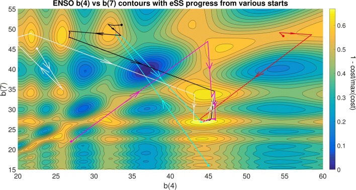
In contrast, we plot the convergence paths of the enhanced scatter search (eSS) method in Fig. 2, showing how the more efficient handling of the local minima allows this strategy to successfully and consistently find the global solution even from initial guesses that are far from the solution. It should be noted that while NIST lists this ENSO problem as being of “average” difficulty, this is largely due to the excellent starting point considered in their test suite, which are extremely close to the solution. Indeed, we can see in the aforementioned figures that the choice of parameter bounds and initial guess can dramatically change the difficulty of the problem.
Fig. 2.
ENSO problem eSS contours: contours of the cost function (nonlinear least squares) for parameters b4 and b7, and trajectories of the enhanced scatter search (eSS) global optimisation solver initialized from various starting points
An automated regularised estimation approach
Here we present a novel methodology, GEARS (Global parameter Estimation with Automated Regularisation via Sampling), that aims to surmount the pitfalls described above. Our method combines three main strategies: i) global optimisation, (ii) reduction of the search space and (iii) regularised parameter estimation. In addition to these strategies, the method also incorporates identifiability analysis, both structural and practical. All these strategies are combined in a hands-off procedure, requiring no user supervision after the initial information is provided.
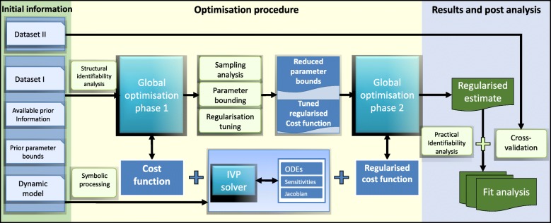
An overview of the entire procedure can be seen in Fig. 3. The initial information required by the method includes the dynamic model to be fitted (as a set of ODEs), the input-output mapping (including the observation function) and a data set for the fitting (dataset I). A second data set is also needed for the purposes of cross-validation and evaluation of overfitting (dataset II). Additionally, users can include (although it is not mandatory) any prior information about the parameters and their bounds. If the latter is not available, users can just declare very ample bounds, since the method is prepared for this worst-case scenario.
Fig. 3.
Workflow of procedure: a schematic diagram of the GEARS method
The method first performs two pre-processing steps. The first is a structural identifiability analysis test. A second pre-processing step involves symbolic manipulation to generate the components needed for the efficient computation of parametric sensitivities. After the pre-processing steps, the method performs a first global optimisation run using eSS and a non-regularised cost function. This step is used to obtain useful sampling information about the cost function landscape, which is then used to perform parameter bounding and regularisation tuning. This new information is then fed into a second global optimisation run, again using eSS but now with a regularised cost function and the new (reduced) parameter bounds. The outcome of this second optimisation is the regularised estimate, which is then subject to several post-fit analysis, including practical identifiability and cross-validation (using dataset II). Details regarding each of these steps are given below.
Structural identifiability analysis
The structural identifiability analysis step allows us to ensure that based on the model input-output (observation) mapping we are considering, we should in principle be able to uniquely identify the parameter values of the model (note that it is a necessary but not sufficient condition). If the problem is found to be structurally non-identifiable, users should take appropriate actions, like model reformulation, model reduction or by changing the input-output mapping if possible.
In our workflow, we analyse the structural identifiability of the model using the STRIKE-GOLDD package [82], which tests identifiability based on the rank of the symbolic Lie derivatives of the observation function. It can then detect each structurally non-identifiable parameter based on rank deficiency.
Symbolic processing for efficient numerics
In GEARS we use a single-shooting approach, i.e. the initial value problem (IVP) is solved for each valuation of the cost function inside the iterative optimisation loop. It is well known that gradient-based local methods, such as those used in eSS, require high-quality gradient information.
Solving the IVP (original, or extended for sensitivities) is the most computationally expensive part of the optimisation, so it is important to use efficient IVP solvers. In GEARS we use AMICI [110], a high level wrapper for the CVODES solver [111], currently regarded as the state of the art. In order to obtain the necessary elements for the IVP solution, the model is first processed symbolically by AMICI, including the calculation of the Jacobian. It should be noted that an additional advantage of using AMICI is that allows the integration of models with discontinuities (including events and logical operations).
Global optimisation phase 1
The objective of this step is to perform an efficient sampling (storing all the points tested during the optimisation) of the parameter space. This sampling will then be used to perform (i) reduction of parameter bounds, and (ii) tuning of the regularisation term to be used in the second optimisation phase.
The cost function used is a weighted least-squares criterion as given by Eqs. (5–7). The estimation problem is solved using the enhanced scatter search solver (eSS, [112]), implemented in the MEIGO toolbox [101]. Within the eSS method, we use the gradient-based local solver NL2SOL [109]. In order to maximise its efficiency, we directly provide the solver with sensitivities calculated using AMICI. After convergence, eSS finds the optimal parameters vector for the fitting data . While this solution might fit the dataset I very well, it is rather likely that it will not have the highest predictive power (as overfitting may have occurred). During the optimization, we store each for function evaluation the parameter vector and its cost value , building the sampling:
| 8 |
| 9 |
where NS is the number of function evaluations, Nθ is the number of parameters and each is a parameter vector selected by eSS.
Parameter bounding
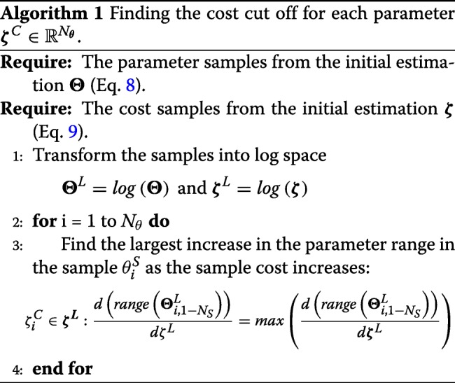
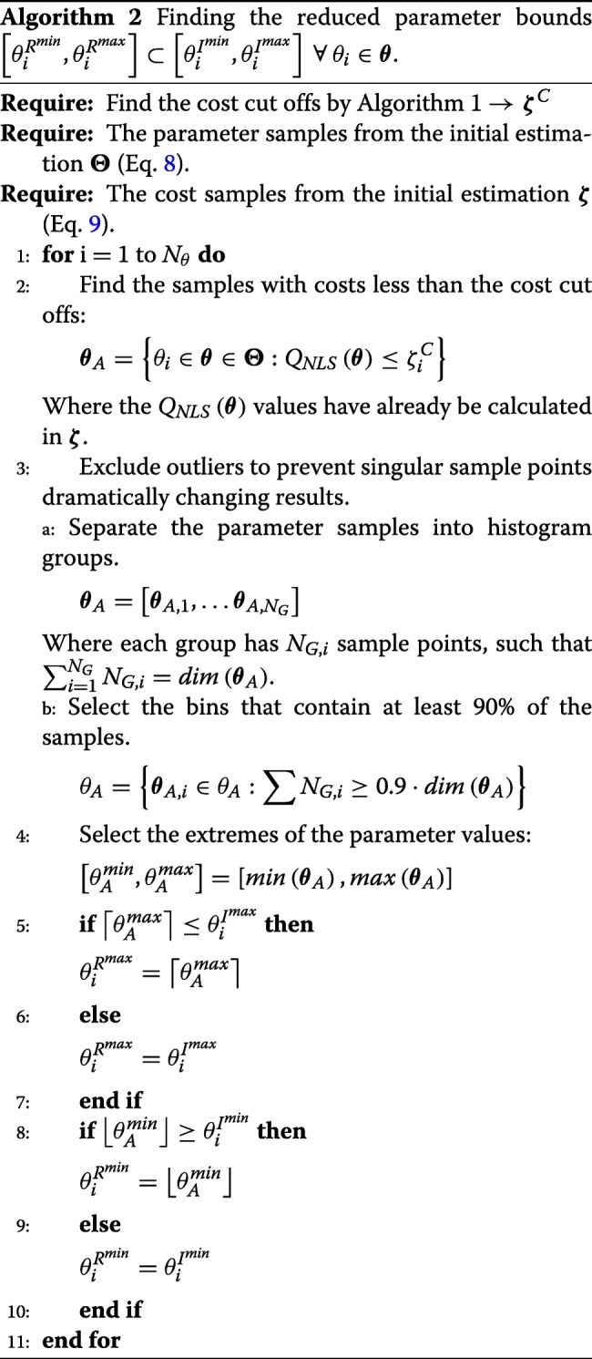
The sampling obtained in the global optimisation phase 1 is now used to reduce the bounds of the parameters, making the subsequent global optimisation phase 2 more efficient and less prone to the issues detailed above. We first compute calculate a cost cut-off value for each parameter using Algorithm 1. This algorithm is used to determine reasonable costs, whereby costs deemed to be far from the global optimum are rejected. We calculate one cost cut off for each parameter, as different parameters have different relationships to the cost function. Once these cut-off values have been calculated for each parameter, we apply Algorithm 2 to obtain the reduced bounds.
Regularised cost function
The next step builds an extended cost function using a Tikhonov-based regularisation term. This is a two norm regularisation term given by:
| 10 |
| 11 |
where W normalises the regularisation term with respect to θref, to avoid bias due to the scaling of the reference parameter. The extended cost function is as follows:
| 12 |
where α is a weighting parameter regulating the influence of the regularisation term.
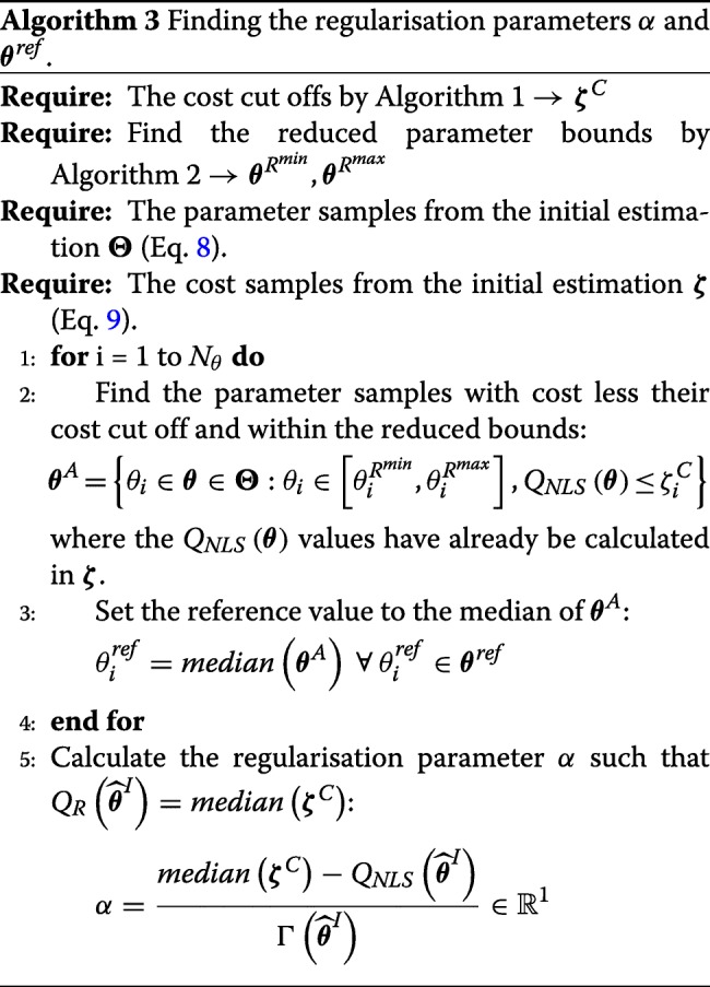
Once the regularised cost function is built, we need to tune the regularisation parameters. Once again, we start from the cost cut off values calculated in Algorithm 2. We also use the reduced parameter bounds to ensure that our regularisation parameters and reduced parameter bounds do not conflict each other. The procedure for calculating the values for the regularisation parameters α and θref can be found in Algorithm 3.
Global optimisation phase 2
Once we have calculated both the values of the regularisation parameters and the reduced parameter bounds, we are now able to perform the final regularised optimisation. We use the same set up for the global optimisation solver (eSS with NL2SOL as the local solver, and AMICI as the IVP solver). We then solve the regularised parameter estimation problem given by:
| 13 |
Subject to the system described in Eqs. 1–3, and the reduced parameter bounds given by:
| 14 |
We denote the solution to this regularised estimation problem as .
Practical identifiability analysis
The next step is to analyse the practical identifiability of the regularised solution. This is done using an improved version of the VisId toolbox [87]. The VisId toolbox accesses practical identifiability based on testing collinearity between parameters. A lack of practical identifiability is typically due to a lack of information in the available fitting data, and in principle can be surmounted by a more suitable experimental design [86].
Cross-validation and post-fit analysis
Next, we assess the level of overfitting using cross-validation. This is typically done by comparing the fitted model predictions with experimental data obtained under conditions (e.g. initial conditions) different from the ones used in the fitting dataset. In other words, cross-validation tests how generalisable the model is. Here, we perform cross-validation on both the non-regularised and regularised solution . This allows us to assess the reduction of overfitting due to the regularised estimation.
In addition to cross-validation, several post-fit statistical metrics are also computed: normalised root mean square error (NRMSE), R2 and χ2 tests [113], parameter uncertainty (confidence intervals computed using the Fisher information matrix, FIM), and parameter correlation matrix (also computed using the FIM). The normalised root mean square error is a convenient metric for the quality of fit, given by:
| 15 |
We use the NRMSE measure to assess both the quality of fit and quality of prediction. One important caveat to note here is that some of these post-fit analyses are based on the Fisher information matrix (FIM) for their calculation. This is a first order approximation and can be inaccurate for highly nonlinear models [114]. In those instances, bootstrapping techniques are better alternatives, although they are computationally expensive.
Implementation: The GEARS Matlab toolbox
The methodology proposed here has been implemented in a Matlab toolbox, “GEARS: Global parameter Estimation with Automated Regularisation via Sampling”. GEARS is a software package that can be downloaded from https://japitt.github.io/GEARS/, made freely available under the terms of the GNU general public license version 3. GEARS runs on Matlab R2015b or later and is multi-platform (tested on both Windows and Linux). The Optimisation and Symbolic Math Matlab toolboxes are required to run GEARS. In addition to this, GEARS requires the freely available AMICI package (http://icb-dcm.github.io/AMICI/) to solve the initial value problem. Optionally, it also requires the Ghostscript software (https://www.ghostscript.com) for improved exportation of results. For more details please see the documentation within the GEARS toolbox. It should be noted that for the structural and practical identifiability analysis steps, users need to install the VisId [87] and STRIKE-GOLDD [82] packages respectively. These packages are freely available at https://github.com/gabora/visid and https://sites.google.com/site/strikegolddtoolbox/ respectively.
Case studies
Next, we consider four case studies of parameter estimation in dynamic models of biological oscillators. The general characteristics of these problems are given in Table 1. While these problems are small in terms the number of parameters, they exhibit most of the difficult issues discussed above, such as overfitting and multimodality, making them rather challenging. For each case study, synthetic datasets (i.e. pseudo-experimental data generated by simulation from a set of nominal parameters) were generated. For each case study, 10 fitting datasets with equivalent initial conditions were produced, plus a set of 10 additional cross-validation data sets (where the initial conditions were changed randomly within a reasonable range). All these data sets were generated using a standard deviation of 10.0% of the nominal signal value and a detection threshold of 0.1.
Table 1.
Summary of case studies considered
| FitzHugh-Nagumo | Goodwin Oscillator | Repressilator | Enzymatic Oscillator | |
|---|---|---|---|---|
| Abbreviation | FHN | GO | RP | EO |
| Main Reference | [117] | [25] | [69] | [116] |
| Number of parameters | 3 | 8 | 4 | 7 |
| Number of estimated parameters | 3 | 8 | 4 | 7 |
| Number of states | 2 | 3 | 6 | 3 |
| Number of observables | 1 | 2 | 1 | 2 |
| Number of data points per experiment | 6 | 20 | 20 | 14 |
FitzHugh-Nagumo (FHN) problem
This problem considers the calibration of a FitzHugh-Nagumo model, which is a simplified version of the Hodgkin-Huxley model [115], describing the activation and deactivation dynamics of a spiking neuron. We consider the FHN model as described by Eqs. 16–21:
| 16 |
| 17 |
| 18 |
| 19 |
| 20 |
| 21 |
where y is the observation function considered in the example. The flexibility of the model dynamics makes this model prone to overfitting. Synthetic data was generated taking nominal parameter values {a,b,g}={0.2,0.2,3}. The fitting data was generated with initial conditions of V0=−1,R0=1.
Goodwin (GO) oscillator problem
The Goodwin oscillator model describes control of enzyme synthesis by feedback repression. The GO model is capable of oscillatory behaviour in particular areas of the parameter space. Griffith [26] showed that limit-cycle oscillations can be obtained only for values of the Hill coefficient n≥8 (note that this information could be used to bound this parameter but here we will not use it, assuming a worst case scenario with little prior information available). The GO model suffers from some identifiability issues as well as tendency to overfitting. The dynamics are given by Eqs. 22–28:
| 22 |
| 23 |
| 24 |
| 25 |
| 26 |
| 27 |
| 28 |
where variables {x1,x2,x3} represent concentrations of gene mRNA, the corresponding protein, and a transcriptional inhibitor, respectively; yF is the observation function for the estimation problem, and yV is the observation function for the cross-validation procedure. Synthetic data was generated considering nominal parameter values {k1−6,Ki,n}={1,0.1,1,0.1,1,0.1,1,10}. The fitting datasets were generated for the initial conditions x1−3,0= [ 0.1,0.2,2.5]. It is important to note that we have considered an additional observable for cross-validation, which makes the problem much more challenging (i.e. it exacerbates the prediction problems due to overfitting).
Repressilator (RP) problem
The Repressilator is a well-known synthetic gene regulatory network [17]. We consider the particular parameter estimation formulation studied by [69] with dynamics given by Eqs. 29–37:
| 29 |
| 30 |
| 31 |
| 32 |
| 33 |
| 34 |
| 35 |
| 36 |
| 37 |
where yF is the observation function for the fitting procedure and yV is the observation function for the cross-validation procedure (i.e. an additional observable for cross-validation). Synthetic data was generated considering nominal parameter values {k1−6,Ki,n}= [ 0.05,298,8.5,0.3]. The fitting data was generated for the initial conditions given by [p1−3,0,m1−3,0]= [ 10,0.01,1,1,0.01,10].
Enzymatic oscillator (EO) problem
The enzymatic oscillator is a small biochemical system model that illustrates the effect of coupling between two instability-generating mechanisms [116]. Parameter estimation in this system is particularly challenging due to the existence of a variety of modes of dynamic behaviour, from simple periodic oscillations to birhythmicity and chaotic behaviour. The chaotic behaviour is restricted to a particular region of the parameter space as discussed in [116]. Its dynamics are difficult even for regions with simple periodic behaviour: the existence of extremely steep oscillations causes small shifts in the period of oscillations to have a large impact on the estimation cost function. We consider the dynamics described by Eqs. 38–43:
| 38 |
| 39 |
| 40 |
| 41 |
| 42 |
| 43 |
where y is the observation function. Synthetic data was generated considering nominal parameter values θ= [ 0.4,500,10,10,0.07,7,2.5]. An important point to note here is that these parameter values were chosen to be in the vicinity of, but not inside, the region with chaotic behaviour. For the fitting datasets the initial conditions [α0,β0,γ0]= [ 29.1999,188.8,0.3367] were used.
Results
All the problems were solved with GEARS using 10 different datasets for fitting and 10 additional datasets for cross-validation. For the RP and GO models an extra observable was considered in the case of the cross-validation. To illustrate the results obtained during the different steps, we will focus on the FHN problem. Detailed results for all the other case studies are given in Additional files 1 and 3. The GEARS software distribution includes all the scripts implementing these case studies.
First, the structural identifiability of these problems was analysed using STRIKE-GOLDD [82], concluding that all of them are identifiable a priori. This analysis also revealed that for the GO case study the initial conditions for the unobserved state x2 must also be known, otherwise two parameters are structurally unidentifiable.
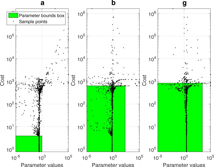
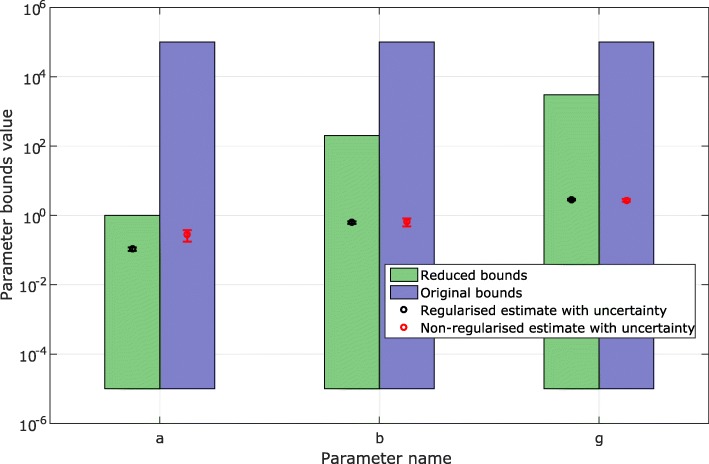
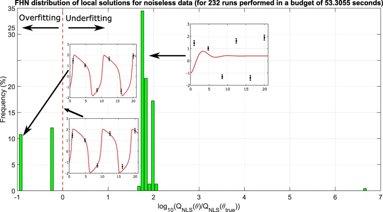
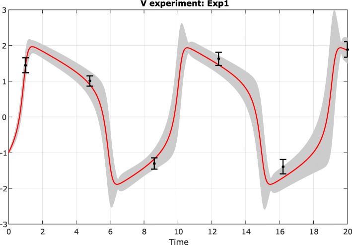
Next, the GEARS workflow proceeded performing an initial estimation. The samples obtained were analysed by applying a cut off to each parameter as seen in Fig. 4 for the FHN problem. The cost cut-off values were then used to significantly reduce the parameter bounds, as shown in Table 2 and Fig. 5. Next, GEARS performed the regularised estimation step (Table 3). We are successful able to avoid the multiple local solutions that are frequently found using local optimisers (see Fig. 6). As expected, this second estimation reduced the quality of the calibration to the fitting data, as shown in Table 4, Figs. 7a and 8. However, it increased the generalisability of the model, as can be seen in Fig. 7 and Table 4. Finally, GEARS confirmed a satisfactory practical identifiability for the resulting calibrated FHN, as indicated by the rather small confidence intervals for the estimated parameters.
Fig. 4.
FHN case study: parameter samples. Parameter samples, showing the cost cut off values and the reduced bounds for each parameter
Table 2.
FHN case study: bounds reduction. A table showing the bounds reduction performed on the FHN model for the first fitting data set
| Parameter | Original bounds | Reduced bounds |
|---|---|---|
| a | [10−5,105] | [10−5,1] |
| b | [10−5,105] | [10−5,1000] |
| g | [10−5,105] | [10−5,100] |
Fig. 5.
FHN case study: reduction of parameters bounds. Original and reduced parameter bounds, also showing the parameter confidence levels for the first fitting data set
Table 3.
FHN case study: summary of the regularised results. A summary of the final results of the procedure applied to the FHN model for the first fitting data set
| Parameter names | Parameter value | Confidence (95%) | Coefficient of variation (%) | Bounds status |
|---|---|---|---|---|
| a | 0.1069 | 0.0129 | 6.1732 | Bounds not active |
| b | 0.6230 | 0.0551 | 4.5130 | Bounds not active |
| g | 2.8490 | 0.1528 | 2.7370 | Bounds not active |
Fig. 6.
FHN case study: distribution of local solutions. Histogram of the local solutions found with a multi-start local solver; the arrows indicate examples of underfitting and overfitting
Table 4.
FHN case study: summary of NRMSE results. A table of the NRMSE for the FHN case study. The fitting is to one particular experiment, while the cross-validation covers ten experiments for the fit to the first fitting data set
| Experiments | Regularised | Non-regularised |
|---|---|---|
| Fitting | 0.2647 | 0.1095 |
| Cross-validation | 1.4054 | 1.4487 |
Fig. 7.
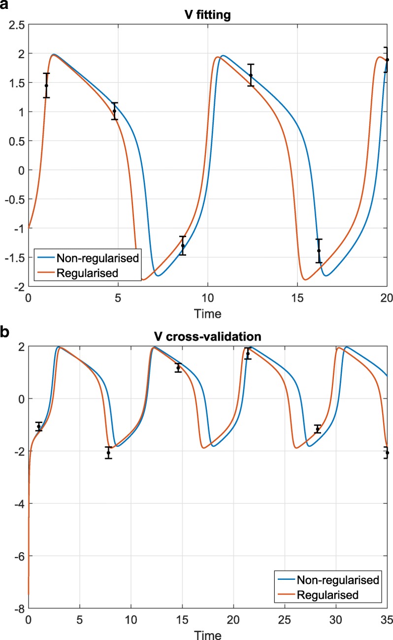
FHN problem: effect of regularisation on fitting and cross-validation. An example of how regularisation affects the calibration of the FHN model: reduction of the quality of the fitting (subplot (a)), but improvement on the quality of the cross-validation (subplot (b)); the corresponding numerical results are given in Table 4
Fig. 8.
FHN problem fit with uncertainty: final regularised fit with uncertainty intervals coonsidering the first fitting data set
More detailed results for FHN and all the other case studies can be found in Additional files 1 and 3. Regarding practical identifiability, using the VisId toolbox we found that both the FHN and RP problems are fully identifiable in practice indicating that our dataset contains enough information. In the case of the EO and GO models we found that there are a number of collinear parameters sets indicating that, at least to some degree, these parameters are compensating one another due to a lack of information in the data.
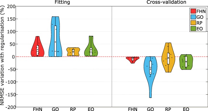
Considering now all the case studies, it is important to assess the consistency of the effect of regularisation on their generalisability. In Fig. 9 we show how the regularised estimation always decreases the quality of calibration to the initial fitting data, as expected. However, the regularised estimations lead to better cross-validation results, i.e. these calibrated models have better predictive power because we have avoided overfitting. It should be noted, however, that there are a few cases where the procedure is unable to significantly improve the generalisability of the model. The explanation is that no real overfit was present in the initial calibrations.
Fig. 9.
Effect of regularisation for all the case studies. Violin plots illustrating the effect of regularisation on the fitting and cross-validation errors (given as normalized root mean square error, NRMSE) for each model and over all the data sets considered. It is shown how regularisation increases the NRMSE for the fitting, but with the benefit of generally improving the predictive power, i.e. reducing the NRMSE in the cross-validations
In summary, using GEARS we have been able to successfully calibrate these challenging oscillators models, avoiding the typical pitfalls, including convergence to local optima and overfitting, in an automated manner.
Conclusions
Parameter estimation in nonlinear dynamic models of biosystems is a very challenging problem. Models of biological oscillators are particularly difficult. In this study, we present a novel automated approach to overcome the most common pitfalls. Its workflow makes use of identifiability analysis and two sequential optimisation steps incorporating three key algorithms: (1) sampling strategies to systematically tighten the parameter bounds reducing the search space, (2) efficient global optimisation to avoid convergence to local solutions, (3) an advanced regularisation technique to fight overfitting.
We evaluate this novel approach considering four difficult case studies regarding the calibration of well known biological oscillators (Goodwin, FitzHugh–Nagumo, Repressilator and a metabolic oscillator). We show how our approach results in more efficient estimations which are able to escape convergence to local optima. Further, the use of regularisation allows us to avoid overfitting, resulting in more generalisable calibrated models (i.e. models with greater predictive power).
Additional files
Remarks on the eSS optimisation solver and detailed results for the Goodwin Oscillator problem and additional ENSO contour plots. This file describes our modifications to the eSS global optimisation solver. It also contains tables and figures showing the detailed results for the Goodwin Oscillator problem, and additional contour plots for the ENSO example. (PDF 1730 kb)
Critical comparison of optimisation solvers. In GEARS, the optimisation problems are solved using the hybrid metaheuristic eSS. A comparison of the eSS global optimisation solver used in GEARS with other competitive local and global optimisation solvers. (PDF 880 kb)
Detailed results for the Fitzhugh-Nagumo, Repressilator and Enzymatic Oscillator problems. This file contains tables and figures showing the detailed results for the Fitzhugh-Nagumo, Repressilator and Enzymatic Oscillator problems. (PDF 1680 kb)
Acknowledgements
Some preliminary results, regarding this study, were presented at the 6th IFAC Conference on Foundations of Systems Biology in Engineering (FOSBE 2016) in Magdeburg, Germany.
Funding
This research has received funding from the European Union’s Horizon 2020 research and innovation program under grant agreement No 675585 (MSCA ITN “SyMBioSys”) and from the Spanish MINECO/FEDER project SYNBIOCONTROL (DPI2017-82896-C2-2-R). Jake Alan Pitt is a Marie Skłodowska-Curie Early Stage Researcher at IIM-CSIC (Vigo, Spain) under the supervision of Prof Julio R. Banga. The funding bodies played no role in the design of the study, the collection and analysis of the data or in the writing of the manuscript.
Abbreviations
- EO
Enzymatic Oscillator model
- eSS
Enhanced scatter search
- FNH
FiztHugh-Nagumo model
- GO
Goodwin Oscillator model
- IVP
Initial value problem
- NIST
National institute of standards
- NLLS
Nonlinear least squares
- RP
Repressilator model
Authors’ contributions
JRB and JAP conceived of the study. JRB planned and coordinated the study. JAP implemented the methods and carried out all the computations. JAP and JRB analysed the results. JRB and JAP drafted the manuscript. All authors read and approved the final manuscript.
Ethics approval and consent to participate
Not applicable.
Consent for publication
Not applicable.
Competing interests
The authors declare that they have no competing interests.
Publisher’s Note
Springer Nature remains neutral with regard to jurisdictional claims in published maps and institutional affiliations.
Footnotes
Availability of data and materials
The datasets supporting the conclusions of this article are available in the GitHub repository https://japitt.github.io/GEARS/. The GEARS toolbox is also freely available at https://japitt.github.io/GEARS/ (10.5281/zenodo.1420464) and is distributed under the terms of the GNU general public license version 3. GEARS runs on Matlab R2015b or later and is multi-platform (Windows and Linux).
Contributor Information
Jake Alan Pitt, Email: jake.pitt@iim.csic.es.
Julio R. Banga, Email: julio@iim.csic.es
References
- 1.Goldbeter A, Lefever R. Dissipative structures for an allosteric model: Application to glycolytic oscillations. Biophys J. 1972;12(10):1302–15. doi: 10.1016/S0006-3495(72)86164-2. [DOI] [PMC free article] [PubMed] [Google Scholar]
- 2.Bier M, Bakker BM, Westerhoff HV. How yeast cells synchronize their glycolytic oscillations: A perturbation analytic treatment. Biophys J. 2000;78(3):1087–93. doi: 10.1016/S0006-3495(00)76667-7. [DOI] [PMC free article] [PubMed] [Google Scholar]
- 3.Danø S, Sørensen PG, Hynne F. Sustained oscillations in living cells. Nature. 1999;402(6759):320–2. doi: 10.1038/46329. [DOI] [PubMed] [Google Scholar]
- 4.Olsen LF, Kummer U, Kindzelskii AL, Petty HR. A model of the oscillatory metabolism of activated neutrophils. Biophys J. 2003;84(1):69–81. doi: 10.1016/S0006-3495(03)74833-4. [DOI] [PMC free article] [PubMed] [Google Scholar]
- 5.Papagiannakis A, Niebel B, Wit EC, Heinemann M. Autonomous metabolic oscillations robustly gate the early and late cell cycle. Mol Cell. 2017;65(2):285–95. doi: 10.1016/j.molcel.2016.11.018. [DOI] [PubMed] [Google Scholar]
- 6.Tyson JJ, Csikasz-Nagy A, Novak B. The dynamics of cell cycle regulation. BioEssays. 2002;24(12):1095–109. doi: 10.1002/bies.10191. [DOI] [PubMed] [Google Scholar]
- 7.Ingolia NT, Murray AW. The ups and downs of modeling the cell cycle. Curr Biol. 2004;14(18):771–7. doi: 10.1016/j.cub.2004.09.018. [DOI] [PubMed] [Google Scholar]
- 8.Alfieri R, Merelli I, Mosca E, Milanesi L. A data integration approach for cell cycle analysis oriented to model simulation in systems biology. BMC Syst Biol. 2007;1. 10.1186/1752-0509-1-35. [DOI] [PMC free article] [PubMed]
- 9.Csikász-Nagy A. Computational systems biology of the cell cycle. Brief Bioinform. 2009;10(4):424–34. doi: 10.1093/bib/bbp005. [DOI] [PubMed] [Google Scholar]
- 10.Barkai N, Leibler S. Circadian clocks limited by noise. Nature. 2000;403(6767):267–8. doi: 10.1038/35002258. [DOI] [PubMed] [Google Scholar]
- 11.Hastings MH. Circadian clockwork: Two loops are better than one. Nat Rev Neurosci. 2000;1(2):143–6. doi: 10.1038/35039080. [DOI] [PubMed] [Google Scholar]
- 12.Rand DA, Shulgin BV, Salazar D, Millar AJ. Design principles underlying circadian clocks. J R Soc Interface. 2004;1(1):119–30. doi: 10.1098/rsif.2004.0014. [DOI] [PMC free article] [PubMed] [Google Scholar]
- 13.Leloup J-C, Goldbeter A. Toward a detailed computational model for the mammalian circadian clock. Proc Natl Acad Sci USA. 2003;100(12):7051–6. doi: 10.1073/pnas.1132112100. [DOI] [PMC free article] [PubMed] [Google Scholar]
- 14.Forger DB, Peskin CS. A detailed predictive model of the mammalian circadian clock. Proc Natl Acad Sci USA. 2003;100(25):14806–11. doi: 10.1073/pnas.2036281100. [DOI] [PMC free article] [PubMed] [Google Scholar]
- 15.Locke JCW, Millar AJ, Turner MS. Modelling genetic networks with noisy and varied experimental data: The circadian clock in arabidopsis thaliana. J Theor Biol. 2005;234(3):383–93. doi: 10.1016/j.jtbi.2004.11.038. [DOI] [PubMed] [Google Scholar]
- 16.Ullner E, Buceta J, Díez-Noguera A, García-Ojalvo J. Noise-induced coherence in multicellular circadian clocks. Biophys J. 2009;96(9):3573–81. doi: 10.1016/j.bpj.2009.02.031. [DOI] [PMC free article] [PubMed] [Google Scholar]
- 17.Elowitz MB, Leibier S. A synthetic oscillatory network of transcriptional regulators. Nature. 2000;403(6767):335–8. doi: 10.1038/35002125. [DOI] [PubMed] [Google Scholar]
- 18.Purcell O, Savery NJ, Grierson CS, Di Bernardo M. A comparative analysis of synthetic genetic oscillators. J R Soc Interface. 2010;7(52):1503–24. doi: 10.1098/rsif.2010.0183. [DOI] [PMC free article] [PubMed] [Google Scholar]
- 19.Kim J, Winfree E. Synthetic in vitro transcriptional oscillators. Mol Syst Biol. 2011;7. 10.1038/msb.2010.119. [DOI] [PMC free article] [PubMed]
- 20.Lu TK, Khalil AS, Collins JJ. Next-generation synthetic gene networks. Nat Biotechnol. 2009;27(12):1139–50. doi: 10.1038/nbt.1591. [DOI] [PMC free article] [PubMed] [Google Scholar]
- 21.El Samad H, Del Vecchio D, Khammash M. Repressilators and promotilators: Loop dynamics in synthetic gene networks. Proceedings of the American Control. 2005;6:4405–4410. [Google Scholar]
- 22.Tsai TY-C, Yoon SC, Ma W, Pomerening JR, Tang C, Ferrell Jr. JE. Robust, tunable biological oscillations from interlinked positive and negative feedback loops. Science. 2008;321(5885):126–39. doi: 10.1126/science.1156951. [DOI] [PMC free article] [PubMed] [Google Scholar]
- 23.Tigges M, Marquez-Lago TT, Stelling J, Fussenegger M. A tunable synthetic mammalian oscillator. Nature. 2009;457(7227):309–12. doi: 10.1038/nature07616. [DOI] [PubMed] [Google Scholar]
- 24.Stricker J, Cookson S, Bennett MR, Mather WH, Tsimring LS, Hasty J. A fast, robust and tunable synthetic gene oscillator. Nature. 2008;456(7221):516–9. doi: 10.1038/nature07389. [DOI] [PMC free article] [PubMed] [Google Scholar]
- 25.Goodwin BC. Oscillatory behavior in enzymatic control processes. Adv Enzym Regul. 1965;3(C):425–4281242943036431437. doi: 10.1016/0065-2571(65)90067-1. [DOI] [PubMed] [Google Scholar]
- 26.Griffith JS. Mathematics of cellular control processes i. negative feedback to one gene. J Theor Biol. 1968;20(2):202–8. doi: 10.1016/0022-5193(68)90189-6. [DOI] [PubMed] [Google Scholar]
- 27.Pavlidis T. Biological Oscillators: Their Mathematical Analysis. New Jersey: Elsevier; 2012. [Google Scholar]
- 28.Strogatz SH. Exploring complex networks. Nature. 2001;410(6825):268–76. doi: 10.1038/35065725. [DOI] [PubMed] [Google Scholar]
- 29.Goldbeter A. Computational approaches to cellular rhythms. Nature. 2002;420(6912):238–45. doi: 10.1038/nature01259. [DOI] [PubMed] [Google Scholar]
- 30.Garcia-Ojalvo J, Elowitz MB, Strogatz SH. Modeling a synthetic multicellular clock: Repressilators coupled by quorum sensing. Proc Natl Acad Sci USA. 2004;101(30):10955–60. doi: 10.1073/pnas.0307095101. [DOI] [PMC free article] [PubMed] [Google Scholar]
- 31.Vasylchenkova A, Mraz M, Zimic N, Moskon M. Classical mechanics approach applied to analysis of genetic oscillators. IEEE/ACM Trans Comput Biol Bioinforma. 2017;14(3):721–7. doi: 10.1109/TCBB.2016.2550456. [DOI] [PubMed] [Google Scholar]
- 32.Stražar M, Mraz M, Zimic N, Moškon M. An adaptive genetic algorithm for parameter estimation of biological oscillator models to achieve target quantitative system response. Nat Comput. 2014;13(1):119–27. doi: 10.1007/s11047-013-9383-8. [DOI] [Google Scholar]
- 33.Rand DA, Shulgin BV, Salazar JD, Millar AJ. Uncovering the design principles of circadian clocks: Mathematical analysis of flexibility and evolutionary goals. J Theor Biol. 2006;238(3):616–35. doi: 10.1016/j.jtbi.2005.06.026. [DOI] [PubMed] [Google Scholar]
- 34.Novák B, Tyson JJ. Design principles of biochemical oscillators. Nat Rev Mol Cell Biol. 2008;9(12):981–91. doi: 10.1038/nrm2530. [DOI] [PMC free article] [PubMed] [Google Scholar]
- 35.Guantes R, Poyatos JF. Dynamical principles of two-component genetic oscillators. PLoS Comput Biol. 2006;2(3):188–97. doi: 10.1371/journal.pcbi.0020030. [DOI] [PMC free article] [PubMed] [Google Scholar]
- 36.Woods ML, Leon M, Perez-Carrasco R, Barnes CP. A statistical approach reveals designs for the most robust stochastic gene oscillators. ACS Synth Biol. 2016;5(6):459–70. doi: 10.1021/acssynbio.5b00179. [DOI] [PMC free article] [PubMed] [Google Scholar]
- 37.Otero-Muras I, Banga JR. Design principles of biological oscillators through optimization: Forward and reverse analysis. PLoS ONE. 2016; 11(12). 10.1371/journal.pone.0166867. [DOI] [PMC free article] [PubMed]
- 38.Kang JH, Cho K-H. A novel interaction perturbation analysis reveals a comprehensive regulatory principle underlying various biochemical oscillators. BMC Syst Biol. 2017;11(1):95. doi: 10.1186/s12918-017-0472-7. [DOI] [PMC free article] [PubMed] [Google Scholar]
- 39.Perez-Carrasco R, Barnes CP, Schaerli Y, Isalan M, Briscoe J, Page KM. Combining a toggle switch and a repressilator within the ac-dc circuit generates distinct dynamical behaviors. Cell Syst. 2018;6(4):521–30. doi: 10.1016/j.cels.2018.02.008. [DOI] [PMC free article] [PubMed] [Google Scholar]
- 40.Strogatz SH, Stewart I. Coupled oscillators and biological synchronization. Sci Am. 1993;269(6):102–1095. doi: 10.1038/scientificamerican1293-102. [DOI] [PubMed] [Google Scholar]
- 41.Henson MA. Modeling the synchronization of yeast respiratory oscillations. J Theor Biol. 2004;231(3):443–58. doi: 10.1016/j.jtbi.2004.07.009. [DOI] [PubMed] [Google Scholar]
- 42.Henson MA. Multicellular models of intercellular synchronization in circadian neural networks. Massachusetts: Elsevier; 2013. [DOI] [PMC free article] [PubMed] [Google Scholar]
- 43.Bold KA, Zou Y, Kevrekidis IG, Henson MA. An equation-free approach to analyzing heterogeneous cell population dynamics. J Math Biol. 2007;55(3):331–52. doi: 10.1007/s00285-007-0086-6. [DOI] [PubMed] [Google Scholar]
- 44.Papachristodoulou A, Jadbabaie A, Munz U. Effects of delay in multi-agent consensus and oscillator synchronization. IEEE Trans Autom Control. 2010;55(6):1471–7. doi: 10.1109/TAC.2010.2044274. [DOI] [Google Scholar]
- 45.Bagheri N, Taylor SR, Meeker K, Petzold LR, Doyle III FJ. Synchrony and entrainment properties of robust circadian oscillators. J R Soc Interface. 2008;5(SUPPL. 1):17–28. doi: 10.1098/rsif.2008.0045.focus. [DOI] [PMC free article] [PubMed] [Google Scholar]
- 46.Gupta A, Hepp B, Khammash M. Noise induces the population-level entrainment of incoherent, uncoupled intracellular oscillators. Cell Syst. 2016;3(6):521–53113. doi: 10.1016/j.cels.2016.10.006. [DOI] [PubMed] [Google Scholar]
- 47.Abel JH, Chakrabarty A, Doyle FJ. Lecture Notes in Control and Information Sciences - Proceedings. Cham: Springer; 2018. Controlling biological time: Nonlinear model predictive control for populations of circadian oscillators. [Google Scholar]
- 48.Sible JC, Tyson JJ. Mathematical modeling as a tool for investigating cell cycle control networks. Methods. 2007;41(2):238–47. doi: 10.1016/j.ymeth.2006.08.003. [DOI] [PMC free article] [PubMed] [Google Scholar]
- 49.Garcia-Ojalvo J. Physical approaches to the dynamics of genetic circuits: A tutorial. Contemp Phys. 2011;52(5):439–64. doi: 10.1080/00107514.2011.588432. [DOI] [Google Scholar]
- 50.Silk D, Kirk PDW, Barnes CP, Toni T, Rose A, Moon S, Dallman MJ, Stumpf MPH. Designing attractive models via automated identification of chaotic and oscillatory dynamical regimes. Nat Commun. 2011; 2(1). 10.1038/ncomms1496. [DOI] [PMC free article] [PubMed]
- 51.Dunlop MJ, Franco E, Murray RM. A multi-model approach to identification of biosynthetic pathways. Proceedings of the American Control Conference. 2007:1600–5. 10.1109/ACC.2007.4282720.
- 52.Podkolodnaya OA, Tverdokhleb NN, Podkolodnyy NL. Computational modeling of the cell-autonomous mammalian circadian oscillator. BMC Syst Biol. 2017;11(1):27. doi: 10.1186/s12918-016-0379-8. [DOI] [PMC free article] [PubMed] [Google Scholar]
- 53.Zak DE, Gonye GE, Schwaber JS, Doyle FJ. Importance of input perturbations and stochastic gene expression in the reverse engineering of genetic regulatory networks: insights from an identifiability analysis of an in silico network. Genome Res. 2003;13(11):2396–405. doi: 10.1101/gr.1198103. [DOI] [PMC free article] [PubMed] [Google Scholar]
- 54.Villaverde AF, Banga JR. Reverse engineering and identification in systems biology: Strategies, perspectives and challenges. J R Soc Interface. 2014; 11(91). 10.1098/rsif.2013.0505. [DOI] [PMC free article] [PubMed]
- 55.Clermont G, Zenker S. The inverse problem in mathematical biology. Math Biosci. 2015;260:11–15. doi: 10.1016/j.mbs.2014.09.001. [DOI] [PMC free article] [PubMed] [Google Scholar]
- 56.Gadkar KG, Gunawan R, Doyle III FJ. Iterative approach to model identification of biological networks. BMC Bioinformatics. 2005;6. 10.1186/1471-2105-6-155. [DOI] [PMC free article] [PubMed]
- 57.Ashyraliyev M, Fomekong-Nanfack Y, Kaandorp JA, Blom JG. Systems biology: Parameter estimation for biochemical models. FEBS J. 2009;276(4):886–902. doi: 10.1111/j.1742-4658.2008.06844.x. [DOI] [PubMed] [Google Scholar]
- 58.van Riel NAW. Dynamic modelling and analysis of biochemical networks: Mechanism-based models and model-based experiments. Brief Bioinform. 2006;7(4):364–74. doi: 10.1093/bib/bbl040. [DOI] [PubMed] [Google Scholar]
- 59.Balsa-Canto E, Alonso AA, Banga JR. An iterative identification procedure for dynamic modeling of biochemical networks. BMC Syst Biol. 2010;4. 10.1186/1752-0509-4-11. [DOI] [PMC free article] [PubMed]
- 60.Jaqaman K, Danuser G. Linking data to models: Data regression. Nat Rev Mol Cell Biol. 2006;7(11):813–9. doi: 10.1038/nrm2030. [DOI] [PubMed] [Google Scholar]
- 61.Chou I-C, Voit EO. Recent developments in parameter estimation and structure identification of biochemical and genomic systems. Math Biosci. 2009;219(2):57–83. doi: 10.1016/j.mbs.2009.03.002. [DOI] [PMC free article] [PubMed] [Google Scholar]
- 62.Geris L, Gomez-Cabrero D, editors. Optimization in Biology Parameter Estimation and the Associated Optimization Problem. Cham: Springer; 2016. [Google Scholar]
- 63.Heinemann T, Raue A. Model calibration and uncertainty analysis in signaling networks. Curr Opin Biotechnol. 2016;39:143–9. doi: 10.1016/j.copbio.2016.04.004. [DOI] [PubMed] [Google Scholar]
- 64.Fan M, Kuwahara H, Wang X, Wang S, Gao X. Parameter estimation methods for gene circuit modeling from time-series mrna data: a comparative study. Brief Bioinform. 2015;16(6):987–99. doi: 10.1093/bib/bbv015. [DOI] [PubMed] [Google Scholar]
- 65.Mhaskar P, Hjortsø MA, Henson MA. Cell population modeling and parameter estimation for continuous cultures of saccharomyces cerevisiae. Biotechnol Prog. 2002;18(5):1010–26. doi: 10.1021/bp020083i. [DOI] [PubMed] [Google Scholar]
- 66.Zwolak JW, Tyson JJ, Watson LT. Parameter estimation for a mathematical model of the cell cycle in frog eggs. J Comput Biol. 2005;12(1):48–63. doi: 10.1089/cmb.2005.12.48. [DOI] [PubMed] [Google Scholar]
- 67.Balsa-Canto E, Peifer M, Banga JR, Timmer J, Fleck C. Hybrid optimization method with general switching strategy for parameter estimation. BMC Syst Biol. 2008;2. 10.1186/1752-0509-2-26. [DOI] [PMC free article] [PubMed]
- 68.Panning TD, Watson LT, Allen NA, Chen KC, Shaffer CA, Tyson JJ. Deterministic parallel global parameter estimation for a model of the budding yeast cell cycle. J Glob Optim. 2008;40(4):719–38. doi: 10.1007/s10898-007-9273-7. [DOI] [Google Scholar]
- 69.Lillacci G, Khammash M. Parameter estimation and model selection in computational biology. PLoS Comput Biol. 2010; 6(3). 10.1371/journal.pcbi.1000696. [DOI] [PMC free article] [PubMed]
- 70.Toni T, Welch D, Strelkowa N, Ipsen A, Stumpf MPH. Approximate bayesian computation scheme for parameter inference and model selection in dynamical systems. J R Soc Interface. 2009;6(31):187–202. doi: 10.1098/rsif.2008.0172. [DOI] [PMC free article] [PubMed] [Google Scholar]
- 71.Wang B, Enright W. Parameter estimation for odes using a cross-entropy approach. SIAM J Sci Comput. 2013;35(6):2718–37. doi: 10.1137/120889733. [DOI] [Google Scholar]
- 72.Vanier MC, Bower JM. A comparative survey of automated parameter-search methods for compartmental neural models. J Comput Neurosci. 1999;7(2):149–71. doi: 10.1023/A:1008972005316. [DOI] [PubMed] [Google Scholar]
- 73.Zak DE, Stelling J, Doyle III FJ. Sensitivity analysis of oscillatory (bio)chemical systems. Comput Chem Eng. 2005;29(3):663–73. doi: 10.1016/j.compchemeng.2004.08.021. [DOI] [Google Scholar]
- 74.Radde N. The impact of time delays on the robustness of biological oscillators and the effect of bifurcations on the inverse problem. EURASIP J Bioinforma Syst Biol. 2009;2009. 10.1155/2009/327503. [DOI] [PMC free article] [PubMed]
- 75.Hafner M, Koeppl H, Hasler M, Wagner A. ’glocal’ robustness analysis and model discrimination for circadian oscillators. PLoS Comput Biol. 2009; 5(10). 10.1371/journal.pcbi.1000534. [DOI] [PMC free article] [PubMed]
- 76.Hasenauer J, Breindl C, Waldherr S, Allgöwer F. Approximative classification of regions in parameter spaces of nonlinear odes yielding different qualitative behavior. Proceedings of the IEEE Conference on Decision and Control. 2010;:4114–9. 10.1109/CDC.2010.5718044.
- 77.Schittkowski K. Numerical Data Fitting in Dynamical Systems: a Practical Introduction with Applications and Software vol. 77. Bayreuth: Springer; 2013. [Google Scholar]
- 78.Seber GAF, Wild CJ. Nonlinear Regression. Wiley Series in Probability and Statistics. Auckland: Wiley; 2003. [Google Scholar]
- 79.Walter E, Pronzato L. Identification of Parametric Models from Experimental Data. London: Springer; 1997. [Google Scholar]
- 80.Chis O-T, Banga JR, Balsa-Canto E. Structural identifiability of systems biology models: a critical comparison of methods. PLoS ONE. 2011;6(11):27755. doi: 10.1371/journal.pone.0027755. [DOI] [PMC free article] [PubMed] [Google Scholar]
- 81.Miao H, Xia X, Perelson AS, Wu H. On identifiability of nonlinear ode models and applications in viral dynamics. SIAM Rev. 2011;53(1):3–39. doi: 10.1137/090757009. [DOI] [PMC free article] [PubMed] [Google Scholar]
- 82.Villaverde AF, Barreiro A, Papachristodoulou A. Structural identifiability of dynamic systems biology models. PLoS Comput Biol. 2016; 12(10). 10.1371/journal.pcbi.1005153. [DOI] [PMC free article] [PubMed]
- 83.Ligon TS, Fröhlich F, Chiş OT, Banga JR, Balsa-Canto E, Hasenauer J. Genssi 2.0: multi-experiment structural identifiability analysis of sbml models. Bioinformatics. 2017;34(8):1421–3. doi: 10.1093/bioinformatics/btx735. [DOI] [PMC free article] [PubMed] [Google Scholar]
- 84.Hong H, Ovchinnikov A, Pogudin G, Yap C. Global identifiability of differential models. arXiv preprint arXiv:1801.08112. 2018.
- 85.Brun R, Reichert P, Künsch HR. Practical identifiability analysis of large environmental simulation models. Water Resour Res. 2001;37(4):1015–30. doi: 10.1029/2000WR900350. [DOI] [Google Scholar]
- 86.Banga JR, Balsa-Canto E. Parameter estimation and optimal experimental design. Essays Biochem. 2008;45:195–209. doi: 10.1042/bse0450195. [DOI] [PubMed] [Google Scholar]
- 87.Gábor A, Villaverde AF, Banga JR. Parameter identifiability analysis and visualization in large-scale kinetic models of biosystems. BMC Syst Biol. 2017; 11(1). 10.1186/s12918-017-0428-y. [DOI] [PMC free article] [PubMed]
- 88.Ljung L, Chen T. Convexity Issues in System Identification.2013. p. 1–9. 10.1109/ICCA.2013.6565206.
- 89.Chen WW, Niepel M, Sorger PK. Classic and contemporary approaches to modeling biochemical reactions. Gene Dev. 2010;24(17):1861–75. doi: 10.1101/gad.1945410. [DOI] [PMC free article] [PubMed] [Google Scholar]
- 90.Mendes P, Kell DB. Non-linear optimization of biochemical pathways: Applications to metabolic engineering and parameter estimation. Bioinformatics. 1998;14(10):869–83. doi: 10.1093/bioinformatics/14.10.869. [DOI] [PubMed] [Google Scholar]
- 91.Esposito WR, Floudas CA. Global optimization for the parameter estimation of differential- algebraic systems. Ind Eng Chem Res. 2000;39(5):1291–310. doi: 10.1021/ie990486w. [DOI] [Google Scholar]
- 92.Moles CG, Mendes P, Banga JR. Parameter estimation in biochemical pathways: A comparison of global optimization methods. Genome Res. 2003;13(11):2467–74. doi: 10.1101/gr.1262503. [DOI] [PMC free article] [PubMed] [Google Scholar]
- 93.Polisetty PK, Voit EO, Gatzke EP. Identification of metabolic system parameters using global optimization methods. Theor Biol Med Model. 2006;3. 10.1186/1742-4682-3-4. [DOI] [PMC free article] [PubMed]
- 94.Geier F, Fengos G, Felizzi F, Iber D. Computational Modeling of Signaling Networks. New Jersey: Springer; 2012. Analyzing and constraining signaling networks: parameter estimation for the user. [DOI] [PubMed] [Google Scholar]
- 95.Raue A, Schilling M, Bachmann J, Matteson A, Schelke M, Kaschek D, Hug S, Kreutz C, Harms BD, Theis FJ, Klingmüller U, Timmer J. Lessons learned from quantitative dynamical modeling in systems biology. PLoS ONE. 2013;8(9):74335. doi: 10.1371/journal.pone.0074335. [DOI] [PMC free article] [PubMed] [Google Scholar]
- 96.Fröhlich F, Kaltenbacher B, Theis FJ, Hasenauer J. Scalable parameter estimation for genome-scale biochemical reaction networks. PLoS Comput Biol. 2017;13(1):1005331. doi: 10.1371/journal.pcbi.1005331. [DOI] [PMC free article] [PubMed] [Google Scholar]
- 97.Rodriguez-Fernandez M, Egea JA, Banga JR. Novel metaheuristic for parameter estimation in nonlinear dynamic biological systems. BMC Bioinformatics. 2006;7. 10.1186/1471-2105-7-483. [DOI] [PMC free article] [PubMed]
- 98.Kim KA, Spencer SL, Albeck JG, Burke JM, Sorger PK, Gaudet S, et al. Systematic calibration of a cell signaling network model. BMC Bioinformatics. 2010;11(1):202. doi: 10.1186/1471-2105-11-202. [DOI] [PMC free article] [PubMed] [Google Scholar]
- 99.Gábor A, Banga JR. Robust and efficient parameter estimation in dynamic models of biological systems. BMC Syst Biol. 2015;9:74. doi: 10.1186/s12918-015-0219-2. [DOI] [PMC free article] [PubMed] [Google Scholar]
- 100.Villaverde AF, Froehlich F, Weindl D, Hasenauer J, Banga JR. Benchmarking optimization methods for parameter estimation in large kinetic models. Bioinformatics. 2018;:bty736. 10.1093/bioinformatics/bty736. [DOI] [PMC free article] [PubMed]
- 101.Egea JA, Henriques D, Cokelaer T, Villaverde AF, MacNamara A, Danciu D-P, Banga JR, Saez-Rodriguez J. Meigo: An open-source software suite based on metaheuristics for global optimization in systems biology and bioinformatics. BMC Bioinformatics. 2014; 15(1). 10.1186/1471-2105-15-136. [DOI] [PMC free article] [PubMed]
- 102.Jaulin L, Walter E. Set inversion via interval analysis for nonlinear bounded-error estimation. Automatica. 1993;29(4):1053–64. doi: 10.1016/0005-1098(93)90106-4. [DOI] [Google Scholar]
- 103.Chachuat B, Houska B, Paulen R, Perić N, Rajyaguru J, Villanueva ME. Set-theoretic approaches in analysis, estimation and control of nonlinear systems. IFAC-PapersOnLine. 2015;28(8):981–95. doi: 10.1016/j.ifacol.2015.09.097. [DOI] [Google Scholar]
- 104.Herrero P, Georgiou P, Toumazou C, Delaunay B, Jaulin L. An efficient implementation of the sivia algorithm in a high-level numerical programming language. Reliab Comput. 2012;16:239–51. [Google Scholar]
- 105.Zamora-Sillero E, Hafner M, Ibig A, Stelling J, Wagner A. Efficient characterization of high-dimensional parameter spaces for systems biology. BMC Syst Biol. 2011;5. 10.1186/1752-0509-5-142. [DOI] [PMC free article] [PubMed]
- 106.Silver N. The Signal and the Noise: Why so Many Predictions Fail–but Some Don’t. New York: Penguin; 2012. [Google Scholar]
- 107.Engl HW, Hanke M, Neubauer A. Regularization of Inverse Problems vol. 375. London: Springer; 1996. [Google Scholar]
- 108.Rogers J, Filliben J, Gill L, Guthrie W, Lagergren E, Vangel M. Strd: Statistical reference datasets for testing the numerical accuracy of statistical software. Technical report, National Institute of Standards and Technology, Washington, D.C. Number 1396. 1998.
- 109.Dennis JE, Gay DM, Walsh RE. An adaptive nonlinear least-squares algorithm. ACM Trans Math Softw (TOMS) 1981;7(3):348–68. doi: 10.1145/355958.355965. [DOI] [Google Scholar]
- 110.Fröhlich F, Theis FJ, Rädler JO, Hasenauer J. Parameter estimation for dynamical systems with discrete events and logical operations. Bioinformatics. 2017;33(7):1049–56. doi: 10.1093/bioinformatics/btw764. [DOI] [PubMed] [Google Scholar]
- 111.Serban R, Hindmash AC. Cvodes, the sensitivity-enabled ode solver in sundials. Proceedings of the ASME International Design Engineering Technical Conferences and Computers and Information in Engineering Conference - DETC2005 6 A. 2005;:257–269.
- 112.Egea JA, Martí R, Banga JR. An evolutionary method for complex-process optimization. Comput Oper Res. 2010;37(2):315–24. doi: 10.1016/j.cor.2009.05.003. [DOI] [Google Scholar]
- 113.Press WH, Teukolsky SA, Flannery BP, Vetterling WT. Numerical Recipes with Source Code CD-ROM 3rd Edition: The Art of Scientific Computing. New York: Cambridge University Press; 2007. [Google Scholar]
- 114.Joshi M, Seidel-Morgenstern A, Kremling A. Exploiting the bootstrap method for quantifying parameter confidence intervals in dynamical systems. Metab Eng. 2006;8(5):447–55. doi: 10.1016/j.ymben.2006.04.003. [DOI] [PubMed] [Google Scholar]
- 115.Hodgkin AL, Huxley AF. A quantitative description of membrane current and its application to conduction and excitation in nerve. J Physiol. 1952;117(4):500–44. doi: 10.1113/jphysiol.1952.sp004764. [DOI] [PMC free article] [PubMed] [Google Scholar]
- 116.Decroly O, Goldbeter A. Proc Natl Acad Sci USA. 1982; 79(22 I):6917–21. 10.1073/pnas.79.22.6917. [DOI] [PMC free article] [PubMed]
- 117.FitzHugh R. Impulses and physiological states in theoretical models of nerve membrane. Biophys J. 1961;1(6):445–66. doi: 10.1016/S0006-3495(61)86902-6. [DOI] [PMC free article] [PubMed] [Google Scholar]
Associated Data
This section collects any data citations, data availability statements, or supplementary materials included in this article.
Supplementary Materials
Remarks on the eSS optimisation solver and detailed results for the Goodwin Oscillator problem and additional ENSO contour plots. This file describes our modifications to the eSS global optimisation solver. It also contains tables and figures showing the detailed results for the Goodwin Oscillator problem, and additional contour plots for the ENSO example. (PDF 1730 kb)
Critical comparison of optimisation solvers. In GEARS, the optimisation problems are solved using the hybrid metaheuristic eSS. A comparison of the eSS global optimisation solver used in GEARS with other competitive local and global optimisation solvers. (PDF 880 kb)
Detailed results for the Fitzhugh-Nagumo, Repressilator and Enzymatic Oscillator problems. This file contains tables and figures showing the detailed results for the Fitzhugh-Nagumo, Repressilator and Enzymatic Oscillator problems. (PDF 1680 kb)


