

Abstract
Estimating the size of stigmatized, hidden, or hard-to-reach populations is a major problem in epidemiology, demography, and public health research. Capture-recapture and multiplier methods are standard tools for inference of hidden population sizes, but they require random sampling of target population members, which is rarely possible. Respondent-driven sampling (RDS) is a survey method for hidden populations that relies on social link tracing. The RDS recruitment process is designed to spread through the social network connecting members of the target population. In this paper, we show how to use network data revealed by RDS to estimate hidden population size. The key insight is that the recruitment chain, timing of recruitments, and network degrees of recruited subjects provide information about the number of individuals belonging to the target population who are not yet in the sample. We use a computationally efficient Bayesian method to integrate over the missing edges in the subgraph of recruited individuals. We validate the method using simulated data and apply the technique to estimate the number of people who inject drugs in St. Petersburg, Russia.
Keywords: hidden population, injection drug use, network inference, population size
1. Introduction
Estimating the size of stigmatized, hidden, or hard-to-reach populations such as homeless people, sex workers, human trafficking victims, men who have sex with men, or drug users is an important part of epidemiological, demographic, and public health research (UNAIDS 2010b, Bao et al. 2010, World Health Organization 2014, Abdul-Quader et al. 2014, Bao et al. 2015, Sabin et al. 2016). Census-like enumeration of hidden population members is usually impossible since potential subjects may fear persecution if they participate in a research study. When random sampling of target population members is feasible, multiplier (e.g. Heimer & White 2010, Hickman et al. 2006, Khalid et al. 2014, Quaye et al. 2015, Thein et al. 2015) and capture-recapture methods (Fienberg 1972, Laska et al. 1988, Larson et al. 1994, Hall et al. 2000, van der Heijden et al. 2015) for estimating population size may perform well. Alternatively, a dynamic model can sometimes be used to link observed population members with the size of the target population (e.g. Kaplan & Soloshatz 1993). Unfortunately random sampling is often impossible because there is no sampling “frame”; population members are not directly accessible to researchers. This difficulty has led researchers to develop survey techniques and corresponding statistical tools that do not require random sampling and instead rely on properties of social networks.
In “snowball sampling”, subjects enumerate their social contacts, each of whom enters the study, and the process repeats (Goodman 1961). Since snowball sampling reveals the network (induced subgraph) of respondents, the sample may carry information about global properties of the social network connecting members of the hidden population. Frank & Snijders (1994) estimate hidden population size from snowball samples by making homogeneity assumptions about the underlying social network, and Dávid & Snijders (2002) use the method to estimate the number of homeless people in Budapest. Further design-based approaches to population size estimation using snowball sampling have been developed (Félix-Medina & Thompson 2004, Félix-Medina & Monjardin 2009, Vincent & Thompson 2012). Snowball sampling is often not feasible because social contacts of participants may decline to enroll in the study. When this happens, the subgraph of respondents may be incomplete, and estimation of population properties - especially the size of the population - may suffer.
The network scale-up method is an alternative technique in which researchers survey members of the general population to determine how many people they know (their personal network size), and how many people they know who are members of the target population (Killworth et al. 1998, Bernard et al. 2010, Shelton 2015). The proportion of respondents’ contacts who are members of the target population is assumed to be equal to the population proportion. Multiplying this proportion by the known general population size produces an estimate of the target population size. The network scale-up method has been successfully used to estimate the size of groups at risk of HIV infection, including men who have sex with men, injection drug users, and sex workers (Kadushin et al. 2006, Salganik et al. 2011, Ezoe et al. 2012, Shokoohi et al. 2012, Guo et al. 2013, Maltiel et al. 2015, Wang et al. 2015, Nikfarjam et al. 2016). The method is appealing because researchers do not need access to the hidden population, but its validity relies on subjects’ knowledge of their contacts’ membership in the target population (Killworth et al. 1998). Sometimes membership in the target population is obscured from non-members (Shelley et al. 1995, 2006), or groups within the general population may have different probabilities of ties to the target population (Snidero et al. 2004, Zheng et al. 2006, McCormick et al. 2010, Feehan & Salganik 2016, Feehan et al. 2016, Maltiel et al. 2015, Habecker et al. 2015).
Respondent-driven sampling (RDS) is a widely used procedure for recruiting members of hard-to-reach populations for surveys and interventions that relies on participants to recruit other subjects (Heckathorn 1997, Broadhead et al. 1998). Beginning with an initial group of participants called “seeds”, subjects are interviewed and given a reward for participation. Subjects then receive a small number of “coupons” that they can use to recruit other eligible subjects. Each coupon is marked with a unique ID traceable back to the recruiter. Subjects recruit others into the study by giving them a coupon that they “redeem” by enrolling in the study. When a new subject enrolls and is interviewed, their recruiter receives a reward. In this way, the RDS recruitment process is designed to spread through the social network of the hidden population. One common feature of all RDS surveys is that researchers assess each subject’s network degree, the number of other members of the target population the subject knows. Because of privacy restrictions, subjects typically do not provide identifying information about members of their social network. Most statistical work on RDS has focused on estimators for population means (Salganik & Heckathorn 2004, Volz & Heckathorn 2008, Gile 2011).
Does RDS reveal information about the size of the target population? Just as in snowball sampling and the network scale-up method, subjects report how many members of the target population they know. Unlike network scale-up surveys, only members of the target population are recruited to participate in an RDS study. In contrast to snowball sampling, not all social contacts of the subject are surveyed: in RDS the subjects decide which of their contacts to recruit. Despite these limitations, Paz-Bailey et al. (2011) use RDS to perform the recapture step of a capture-recapture experiment, even though recruitment does not constitute a probability sample from the target population (see Berchenko & Frost 2011, for commentary). Recently Handcock, Gile & Mar (2014) and Handcock et al. (2015) proposed a population size estimator for RDS based on ideas from without-replacement sampling proportional to size (Bickel et al. 1992, Gile 2011). Their successive sampling size (SS-size) estimator depends only on the time-ordered sequence of observed network degrees in the RDS sample. By assuming that RDS is a sampling mechanism that recruits individuals without replacement and with probability proportional to their network degree, Handcock, Gile & Mar (2014) and Handcock et al. (2015) reason that the average degrees of recruited individuals should decrease monotonically with the number of recruited subjects. The rate of this decrease is believed to reveal information about the size of the population via early depletion of high-degree individuals (see, e.g. Wesson et al. 2015, Johnston et al. 2015, 2016). The RDS Analyst software implements the SS-size method (Handcock, Fellows & Gile 2014).
In this paper, we take a network-based approach to population size estimation from RDS, based on the intuition behind the snowball sampling estimator and the network scale-up method. The key insight is that the RDS recruitment chain, timing of recruitments, and the degrees of recruited subjects provide information about the number of links between sampled and unsampled population members, and hence the total population size. We first describe the graphical structure of data obtained from RDS, including the recruitment graph and recruitment-induced subgraph. The unobserved portions of the recruitment-induced subgraph are treated as missing data. We describe a Bayesian framework for marginalizing over the missing edges in the recruitment-induced subgraph to estimate population size. The method relies only on data traditionally obtained by RDS and does not require a change to current RDS recruitment protocol, nor a separate survey of subjects who are not members of the target population. The computational burden of the inference procedure scales with the sample size, not the total hidden population size. We validate the proposed technique using simulated data and apply the method to estimate the number of injection drug users in St. Petersburg, Russia.
2. The graphical structure of RDS data
In this section, we outline the observed data in typical RDS surveys of hidden populations, drawn from the definitions given by Crawford (2016). Suppose that the hidden population social network is G = (V,E), where |V| = N is the size of the target population and G contains no self-loops or parallel edges. A vertex in G is recruited if it is known to the study. A recruited vertex cannot be recruited again.
Definition 1 (Recruitment graph).
The directed recruitment graph is GR = (VR, ER), where VR ⊂ V is the set of n sampled vertices and a directed edge {i,j} ∈ ER indicates that i recruited j.
Since subjects cannot be recruited more than once, Gr is acyclic.
Definition 2 (Degree).
A vertex’s degree is the number of edges incident to it that connect to vertices in the hidden population graph G.
Definition 3 (Recruitment-induced subgraph).
The recruitment-induced subgraph is an undirected graph GS = (VS,ES), where VS = VR consists of the n sampled vertices, and {i,j} ∈ ES if and only if i ∈ VS, j ∈ VS, and {i,j} ∈ E.
Let d = (d1,...,dn) be the time-ordered n × 1 vector of subjects’ degrees in G, according to Definition 2, in the order they were recruited into the study. Let t = (t1,...,tn) be the n × 1 vector of recruitment times, where t1 < · · · < tn.
Definition 4 (Coupon matrix).
Let C be the n × n coupon matrix whose element Cij is 1 if subject i has at least one coupon just before the jth recruitment event, and zero otherwise. The rows and columns of C are ordered by subjects’ recruitment time.
The observed data from the RDS recruitment process is Y = (GR, d, t, C). Figure 1 illustrates the observed data and their relationship to the unobserved population graph G. Since the recruitment graph GR does not contain any edges along which a recruitment event did not take place, the recruitment-induced subgraph GS is not fully observed. However, the observed degrees d and the edges in the recruitment graph GR place restrictions on the number of non-recruitment edges that can connect vertices in VS, so an estimate of GS must adhere to certain compatibility conditions.
Figure 1:
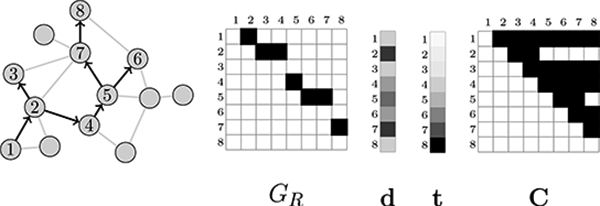
Illustration of the observed data in RDS surveys. At left, the recruitment graph GS is shown overlaid on the population graph G. Next the observed data are shown: the adjacency matrix of the recruitment graph GR, the vector of recruited vertex degrees d in G, the vector of recruitment times t, and the coupon matrix C. The numbered rows and columns correspond to the sampled vertices, in the order of their recruitment. Each subject received 2 coupons, so subjects 2 and 5 deplete their coupons before the end of the study. This figure is adapted from Crawford (2016).
Definition 5 (Compatibility).
An estimated subgraph is compatible with the observed data (GR, d) if the following conditions are met: 1. the vertices in the estimated subgraph are identical to the set of recruited vertices: if and only if 2. all directed recruitment edges are represented as undirected edges: for all (i,j) ∈ ER, ; 3. the number of edges in GS belonging to each sampled vertex does not exceed the vertex’s degree: for all , , where dv is the degree of vertex v.
These compatibility conditions provide topological constraints on the structure of .
3. Estimating the population size
We now construct a probability model by which the observed data Y = (GR, d, t, C) in an RDS survey are linked to the number of vertices N in the target population. Figure 2 illustrates the problem of estimating the number of vertices N in G from the recruitment-induced subgraph GS. First we show that if the recruitment-induced subgraph GS is known, a simple statistic - the number of pendant edges connecting each sampled vertex to unsampled vertices at the moment of recruitment - can be used to derive the likelihood of N conditional on GS. Next, we appeal to results by Crawford (2016) giving the likelihood of the recruitment-induced subgraph GS and a per-edge recruitment rate parameter λ. Our strategy is to marginalize over the unknown recruitment-induced subgraph to estimate N.
Figure 2:
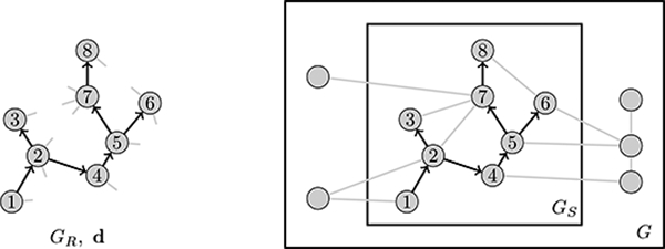
Illustration of population size estimation task from RDS data. We seek the number of vertices in G. The observed recruitment graph GR is shown at left, along with pendant edges implied by observed vertex degrees. At right, the reconstructed subgraph GS reveals the number of edges that connect to unsampled vertices at each step of the recruitment process.
3.1. Likelihood of N given GS under the Erdős-Rényi model
We first state some assumptions about the social network connecting members of the hidden population and the RDS recruitment process on this network.
Assumption 1 (Existence of a network).
The target population social network is a finite graph G = (V, E) with no parallel edges or self-loops.
Network-based methods for population inference must make homogeneity assumptions to ensure that a sub-sample of the network can be used to make inference about the total network. In the Erdős-Rényi random graph model, each edge between vertices is formed independently with probability p (Erdős & Rényi 1959, 1960). Let denote an Erdős-Rényi random graph. The degree di of a vertex i has distribution
| (1) |
where N = |V|. The likelihood of a particular graph G depends only on the number of edges |E|,
| (2) |
The Erdős-Rényi random graph model formalizes the notion of independent and identically distributed (with probability p) formation of reciprocal social ties between individuals in a finite population. While the Erdős-Rényi model is believed to be a poor generative model for non-hidden social networks (Watts & Strogatz 1998, Robins et al. 2001), very little is known about the structure of contacts between members of highly stigmatized or criminalized populations. The Erdős-Rényi model has proven to be empirically useful for estimating hidden population sizes: both the snowball sampling estimator (Frank & Snijders 1994) and the network scale-up estimator (Killworth et al. 1998) rely on equivalent network homogeneity assumptions.
Assumption 2 (Network model).
The target population graph has Erdős-Rényi distribution, .
The likelihood of GS conditional on GR and d under the Erdős-Rényi model depends on assumptions about the dynamics of the RDS recruitment process. But there is significant disagreement about how to model the recruitment process (Salganik & Heckathorn 2004, Gile & Handcock 2010, Gile 2011, Berchenko et al. 2013, Crawford 2016, Malmros et al. 2014). We therefore make a simple assumption that permits calculation of the distribution of a statistic of GS under Assumption 2. Call a vertex a recruiter if it has at least one coupon and shares an edge with an unrecruited vertex. Call a vertex susceptible to recruitment if it has not yet been recruited and shares an edge with a recruiter.
Assumption 3 (RDS conditional sampling probabilities).
The next recruited vertex is chosen from among all susceptible vertices with probability that depends only on the edges it shares with recruiters. The edges connecting the newly recruited vertex to other unrecruited vertices do not affect its probability of being recruited.
Assumption 3 provides a connection between the recruitment probability for each vertex and the structure of the network.
Under Assumptions 2 and 3, the recruitment-induced subgraph GS is not an Erdős-Rényi graph because new recruits may not be chosen uniformly at random from the set of unrecruited vertices. However, since recruitment probability does not depend on edges not connected to active recruiters, it does not depend on edges connecting unrecruited vertices to other unrecruited vertices in particular. This intuition yields a suitable probability model linking the subgraph GS to the population size N. Let be the number of edges belonging to vertex i that connect to unknown vertices at the moment i is recruited (recall that the indices i are ordered by the time of entry into the study),
| (3) |
Then by independence of edges in the Erdős-Rényi model,
| (4) |
unconditional on di and dj for j ≠ i and for j ≠ i. In words, the number of edges connecting a recruited vertex to unrecruited vertices (at the moment it is recruited, before observing its total degree) depends only on the number of remaining unrecruited vertices and p, where we have not conditioned on any other observables. The presence of the population size parameter N in (4) suggests that the sequence of ‘s may contain information about N. Since are assumed to be independent binomial random variables, the joint likelihood of N and p, given GS and d, is
| (5) |
where is calculated from knowledge of GS and d via (3).
3.2. Likelihood of GS
The likelihood (5) permits estimation of N, conditional on observation of the recruitment-induced subgraph GS. However, GS is not directly revealed by the observed data Y. The statistic is sufficient for N and p, but the graphical structure of GS induces complex combinatorial dependencies in the elements of du, and the marginal probability distribution of du cannot be represented in a simple way. We therefore seek a probability model for GS given Y, and marginalize over the unobserved portion of this graph with respect to this model. The compatibility conditions given in Definition 5 place strong restrictions on the structure and density of GS. Let C(GR, d) denote the set of all recruitment-induced subgraphs that are compatible with the observed data GR and d.
The least restrictive option is to marginalize over GS with respect to the uniform distribution on C(GR, d) by setting Pr(GS|Y) α 1 for GS ∈ C(GR, d) and zero otherwise. However, the uniform distribution over C(GR, d) does not give rise to the uniform distribution over |ES|, and most subgraphs in C(GR, d) have far more edges than the true subgraph GS. The result is that the uniform distribution over subgraphs GS results in a highly informative distribution over du that does not place most of its mass near the true value of du. A more sophisticated marginalizing distribution can be derived from the time series of recruitment events. By making assumptions about the time dynamics of the recruitment process on GS, we can calculate the likelihood of the observed recruitment times t conditional on GS to develop a probability model for GS. The recruitment model depends on the following assumptions, drawn directly from Crawford (2016).
Assumption 4.
Vertices become recruiters immediately upon entering the study and receiving one or more coupons. They remain recruiters until their coupons or susceptible neighbors are depleted, whichever happens first.
Call an edge in G susceptible if it links a recruiter and a susceptible vertex.
Assumption 5.
When a susceptible neighbor j of a recruiter i is recruited by any recruiter, the edge connecting i and j is immediately no longer susceptible.
Assumption 6 (Exponential waiting times).
The time to recruitment along an edge connecting a recruiter to a susceptible neighbor has exponential distribution with rate λ, independent of the identity of the recruiter, neighbor, and all other waiting times.
Assumptions 4–6 are consistent with Assumption 3 (for proof, see Propositions 1 and 2 of Crawford 2016). Thompson (2006) gives a nearly equivalent characterization of adaptive web sampling in which edges connected to an “active set” of units (recruiters) can be followed to reveal additional units (susceptible vertices).
The likelihood of the recruitment time series on a fixed graph can be computed under this model. Let w = (0, t1 - 0, t2-t1,...,tn-tn-1) be the vector of inter-recruitment waiting times. Let A be the adjacency matrix of GS, where the rows and columns of A correspond to vertices in the order of their recruitment into the study. Let u be the n × 1 vector whose ith element is the number of pendant edges emanating from i to unsampled vertices, . Then the joint likelihood of GS and the waiting time parameter λ is given by
| (6) |
where
| (7) |
C is the coupon matrix, and M is the set of seeds (Crawford 2016). Information from the subgraph GS enters the likelihood through the vector statistic s, the number of susceptible edges just before each recruitment event.
3.3. Posterior distribution of N
We now combine the likelihood expressions (5) and (6) with prior information to estimate the posterior distribution of N given the observed data Y. Assume N, p, GS, and λ are a priori independent with prior distributions π(N), π(p), π(GS), and π(λ) respectively. Traditional Gibbs sampling is impossible since the conditional posterior Pr(N,p|GS, λ, Y) contains an intractable normalizing constant that depends on N and p; sampling from this distribution is prohibitively difficult. This problem arises often in estimation of parameters given a realization from a random graph model (see, e.g. Hunter & Handcock 2006).
Since we do not seek the joint posterior over all unknowns, and instead wish only to find the marginal distribution of N, we first conduct Bayesian inference on GS. For each sample from the distribution of GS|Y, we can compute the statistic , and we can sample from the posterior (predictive) value of N given . We first write the posterior distribution of GS and λ given Y, Pr(GS, λ|Υ) = L(GS, λ; Y)π (GS)π(λ)/κ(Υ), where κ(Υ) is a normalizing constant. Note that Pr(GS, λ| Y) is not the “marginal” posterior distribution over N and p, but the posterior distribution of GS and λ alone given Y. Likewise, we can write the distribution of N and p given GS and Y as Pr(N,p|GS, Y) = L(N,p; GS, Y)π(N)π(p)/k(Gs, Y) where k(Gs, Y) is a normalizing constant and Nmin = n+maxi di is the minimum value of N, described in detail below. The posterior (predictive) distribution is obtained by marginalizing over compatible subgraphs, p, and λ,
| (8) |
Let p have Beta(α,β) distribution with density π(p) = pα−1(1 — p)β−1/B(α,β) where B(·, ·) is the Beta function. Let λ have Gamma(n,ξ ) distribution with density π(λ) =ξn λη−1e-ξλ/Γ(η) where Γ(·) is the Gamma function. Then integrating analytically over p and λ in (8), the posterior (predictive) distribution of N becomes
| (9) |
where and s are computed using . A derivation of (9) is given in the Supplementary Materials.
3.3.1. Prior distributions for N
Not every value of N is feasible: since no parallel edges are allowed under Assumption 1, N must be large enough to accommodate all the edges emanating from sampled vertices. Therefore, we need for the s derived from a particular subgraph . Rather than make the prior π(N) conditional on each particular realization of , we note that for every compatible and impose the simpler constraint N ≥ n + maxi di, which does not depend on any particular . For surveys where N ≫ n, this should not pose a problem for estimation of N. Setting Nmin = n + maxi di, we will always consider (8) to be defined only for N ≥ Nmin.
A relatively uninformative class of prior distributions for N is the power-law mass function π(N) α N-c where c ≥ 0 and N ≥ Nmin. When c > 1 the prior density is proper: When c > 2 the prior mean exists, and when c > 3 the prior variance exists. However, researchers may prefer not to specify a strongly informative prior for N, and c = 1 is a popular choice (Draper & Guttman 1971, Raftery 1988). Unfortunately the distribution Pr(N|Y) may not behave well for some values of c: Kahn (1987) warns that estimates based on the beta-binomial distribution can have undesirable properties under some priors π(N). In the Supplementary Materials, we show that the mass function (8) is a proper probability distribution when α + c > 1; when α + c > 2 the posterior mean is finite, and when α + c > 3 the posterior variance is finite. When posterior moments of interest do not exist, it may be tempting to posit Nmax, the largest permissible estimate of N, and letting . But since the posterior moments for unbounded N are undefined, their estimates under the truncated prior depend acutely on the choice of Nmax and are less influenced by the observed data (Kahn 1987). We therefore consider below specifications of π(N) such that the prior has infinite support, the posterior is proper, and at least the first two moments exist. While this inevitably results in a more informative set of priors, it seems a small price to pay for finite posterior mean and variance.
3.4. Monte Carlo sampling
The distribution (8) is obtained by marginalizing over compatible subgraphs . Under the compatibility conditions in Definition 5, this sum cannot be performed analytically and the distribution of N conditional on does not have a standard form. Furthermore, the normalizing constants k(Y) and k(, Y) are unknown. We therefore resort to Monte Carlo sampling to perform this marginalization. First we sample |Y, then sample N conditional on . Sampling is efficient because update expressions are available for the statistic s in the likelihood (6), making the matrix multiplications in (7) unnecessary. Integration over compatible subgraphs is accomplished by proposing changes to the connectivity of , then using a Metropolis-Hastings step to accept or reject the proposal. Sampling N given relies on a close approximation to the conditional posterior distribution. The Supplementary Materials provide a comprehensive description of the sampling algorithm.
4. Validation using simulated data
We performed simulations to validate the proposed method for population size estimation from RDS data under the model outlined in Section 3. First, we simulate an Erdos-Rényi population network G = (V,E) with |V| = N = 5000, 10000, and 100000, p = 5/N, 10/N, and 20/N. Conditional on the simulated population graph, we simulate the RDS recruitment process under typical real-world study conditions with n = 500 recruitments starting from |M| = 10 seeds chosen at random, and three coupons per recruit using the model described by Crawford (2016). This yields simulations with realistic - and small - sample fractions n/N of 10%, 5%, and 0.5%. From the simulated recruitment data, we extract Y = (Gr, d, t, C) and estimate the distribution of N given Y as outlined above.
We employ weakly informative priors for the unknown parameters. We assign to N the vague improper prior distribution . For the edge density p we assign p ~ Beta(α,ß), with α > 2 and β = α(1 — ptrue)/ptrue, where ptrue is the true value of p. This specification ensures that the distribution of N has finite second moment and the prior expectation of p is equal to ptrue. To evaluate the sensitivity of estimates to variation in the prior parameters, we set α = 3, 5, and 10; we set the prior variance for λ to νλ = 1, since simulation results appear to be insensitive to the prior variance for λ. The prior for GS is where γ = log (ptrue/(1 — ptrue)). For the waiting time parameter λ, we specify η and ξ to give prior mean equal to the true value λtrue and prior variance νλ. Then we let and ξ = Atrue/vλ, which gives Ε[λ] = λtrue and Var[λ] = νλ. The true value is λtrue = 1 for all simulations.
For each parameter combination, we simulated 10 independent networks and RDS datasets, and for each dataset, we estimate the distribution of N. Figure 3 shows summaries on the relative error scale, (. For N = 5000 estimates exhibit small positive bias in the posterior mean, due to the heavy-tailed prior and the fact that the support of N is bounded below at Nmin and unbounded above, since we do not specify a maximum value for N. This relative error is attenuated for larger population size (and smaller sample fraction). The posterior mode usually under-estimates the true value of N slightly, with this relative error decreasing with increasing N, (N — 1)p, and prior precision. Estimates of N exhibit least bias when a is large, indicating greater certainty about the edge density p.
Figure 3:
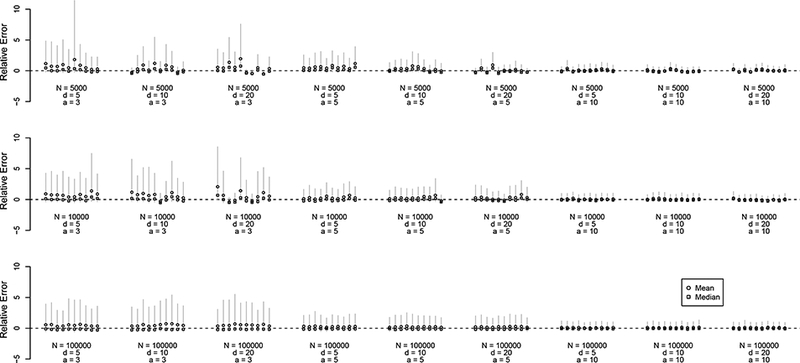
Estimates of N from simulated data, on the relative error scale . Networks were simulated with N ∈ {5000,10000,100000} and d ∈ {5,10, 20}. RDS data were simulated with n = 500, |M| = 10, λ = 1. The prior mean of p was set to the true value of p, and increasing values of α ∈ {3, 5,10} result in smaller prior variance for p. Circles indicate posterior means, squares indicate posterior modes, and gray vertical lines indicate 95% posterior quantiles for N.
In the Supplementary Material, we also provide estimation results for simulated data under three types of mis-specification. First, we evaluate estimates of N when the prior mean of p is not equal to the true value ptrue used in simulations. The vague improper prior and the requirement that the posterior distribution of N have finite first and second moments necessitate a somewhat informative prior for p. We consider simulations in which Επ[p] = fptrue and π(Gs) exp[-γ|Es|] where γ = log (fptrue/(1 - fptrue)), where f > 0 is the mis-specification fraction. Serious mis-specification of the prior mean Eπ [p] of p has a predictable effect on the relative error. When 0 < f < 1, N is usually over-estimated; when f > 1, N is usually under-estimated. As expected, the magnitude of this error is greatest when / is much smaller than 1, since N is unbounded above. In most cases, the 95% posterior quantile intervals for N still cover the true value of N used in the simulation. Second, we investigate estimates under mis-specification of the underlying population network model. We construct a two-group stochastic blockmodel similar to that employed by Handcock, Gile & Mar (2014) in evaluation of the SS-size method. In each block, within-block connection probabilities are equal. Between-block connection probabilities are varied under the constraint that the expected total number of edges in the network remain constant at . This simulation setup investigates the sensitivity of estimates to block structure in the underlying network, but the expected number of edges is equal to the value expected under the Erdôs-Rényi assumption. The results indicate that the proposed method is relatively insensitive to block structure alone. Third, we study estimates under similar network mis-specification, but with unequal within-block connection probabilities and constant expected total number of edges. In this situation, one block may have far more edges than the other; depending on the size of the block with more edges and its edge density, positive bias can result. Vertices in this small block are unlikely to be chosen as seeds, but most of the edges in the graph reside in this block. Vertices in the larger block are most likely to be chosen as seeds, but these and other vertices in the larger block have few edges and small degree. Positive bias is exhibited when a block comprising a small fraction of vertices is nearly complete. Crawford (2016) studies accuracy of estimation of under violation of Assumption 6.
5. Application: how many people inject drugs in St. Petersburg?
The Russian Federation has experienced simultaneous epidemics of drug abuse and HIV infection since the mid-1990s, and HIV prevalence is highest among people who inject drugs (PWID) (Abdala et al. 2003, Rhodes et al. 2004, World Health Organization 2005, Pokrovsky et al. 2010, UNAIDS 2010a). Drug possession in Russia can result in serious legal penalties, including incarceration, loss of employment, and revocation of driving privileges. HIV-positive people in Russia are often subject to strong social stigma and may lack access to treatment and education resources (Balabanova et al. 2006, Sarang et al. 2012, Burke et al. 2015). In St. Petersburg, Russia, HIV incidence and prevalence are high among PWID (Kozlov et al. 2006, Niccolai et al. 2011), and researchers have found that many PWID do not have ready access to HIV testing and are not aware of their HIV status (Niccolai et al. 2010). PWID in Russia often obtain drugs through local social networks connecting drug dealers and buyers (Shaboltas et al. 2006, Cepeda et al. 2011). The social nature of the drug scene in St. Petersburg creates problems for public health and epidemiological research on PWID (also called injection drug users - IDUs): “Such a structure makes it difficult to recruit through outreach and easier to recruit by allowing IDUs to penetrate their own network of contacts” (Shaboltas et al. 2006, page 662). PWID in St. Petersburg therefore constitute an epidemiologically important hidden population, connected by a social network, for which random sampling is impossible.
Knowledge of the size of the PWID population in St. Petersburg would substantially illuminate the number of people at risk for HIV infection, and could help determine the scale and scope of education, treatment, and intervention programs in that community. To estimate the number N of PWID in St. Petersburg, Heimer & White (2010) use a multiplier method with estimated HIV prevalence (from a different RDS study), HIV testing frequency, and other sources of information to obtain = 83118 ± 5799. Given that nearly all epidemiological research on PWID in St. Petersburg uses RDS to recruit participants, a method for estimating population size directly from RDS data would be particularly useful.
We analyze data from an RDS study of PWID in St. Petersburg performed during 2012–2013. Researchers recruited n = 813 PWID using 17 seeds and conducted interviews to gauge perceived barriers to use of HIV prevention and treatment services. While the study was not intended to be used for population size estimation, its size and adherence to the traditional RDS recruitment protocol outlined by Heckathorn (1997) make it an appealing opportunity for population size estimation. Crawford (2016) shows the observed data Y = (Gr, d, t, C) from this study and describes the recruitment procedure in detail.
We investigate estimation of N under the vague prior π(Ν)N−1, λ ~ Gamma(n = 1,ξ = 1), and several specifications for π(p), indexed by the parameters α and β. To find a suitable prior for p that takes into account both the previous population size estimate of Heimer & White (2010) and the requirement that the first two moments of the posterior distribution exist, we adopt an empirical Bayes approach. In the Supplementary Materials, we describe a method for prior elicitation using a lower bound for p, given a prior estimate N of N. For the St. Petersburg data, we find that this bound is . We fix different values of α ≥ 2.1 and choose β > 0 such that Pr(p > plo|α,ß) = 0.99 under the Beta distribution for p. We consider α = 2.1,3,..., 10, and as before, we set , with.
Table 1 shows summaries for the estimated number N of PWID in St. Petersburg under each prior specification. The mode, mean, standard deviation (SD), and 95% quantiles are shown. For reference, Heimer & White (2010) state that at least 30,000 cases of HIV in PWID have been reported; the 2.5% quantiles for α = 2.1 and 3.0 are just below this number, but all posterior modes and means exceed it. Under this prior specification, increasing values of a decrease the prior mean of p, giving larger posterior estimates and variances of N. The posterior mean E[N|Y] is more sensitive than the mode to changes in a because it is strongly affected by the thickness of the right-hand tail of the posterior distribution. We obtain posterior mode estimates between 39,000 and 215,000, which are generally compatible with that of Heimer & White (2010): most posterior quantile intervals computed here contain their estimate = 83,118. Setting α =10 results in the highest estimates of over 200,000; estimates substantially larger than this may not be credible. The total number of people in St. Petersburg is approximately 4.9 million, and Heimer & White (2010) estimate the number who match the age range (20–45 years) characteristic of PWID as approximately 1.5 million. The last two columns give the implied prevalence of injection drug use in both of these groups, computed using the posterior mean. Posterior expectations and quantiles of N in Table 1 are sensitive to the prior mean of p. The conditions required for the posterior distribution of N to have finite variance necessitate informative priors for p (Kahn 1987); dramatic mis-specification of the prior mean of p can result in bias, as we show in the Supplementary Material. Nevertheless, the estimates of the number N of PWID in St. Petersburg are in general agreement with those of Heimer & White (2010) and span a range of reasonable values. Figure 4 shows posterior density estimates for each value of α that appears in Table 1.
Table 1:
Estimates of the number of people who inject drugs in St. Petersburg, Russia from an RDS dataset of n = 813 subjects. Posterior means, standard deviations, and 2.5% and 97.5% quantiles are shown. The last two columns show the approximate implied prevalence (%) of injection drug use in 20–45 year-olds and for all residents of St. Petersburg.
| Prior |
Population size N |
Prevalence (%) | |||||
|---|---|---|---|---|---|---|---|
| α | Mode | Mean | SD | 2.5% | 97.5% | 20–45yrs | All |
| 2.1 | 39327 | 87678 | 104925 | 19659 | 340769 | 5.8 | 1.8 |
| 3.0 | 52466 | 104449 | 126935 | 29384 | 351413 | 7.0 | 2.1 |
| 4.0 | 81875 | 129420 | 92224 | 43098 | 382347 | 8.6 | 2.6 |
| 5.0 | 109548 | 150977 | 83846 | 60050 | 366760 | 10.1 | 3.1 |
| 6.0 | 126296 | 174442 | 85028 | 75391 | 385644 | 11.6 | 3.6 |
| 7.0 | 146483 | 193728 | 84272 | 90074 | 409119 | 12.9 | 4.0 |
| 8.0 | 170293 | 216841 | 91180 | 104725 | 441624 | 14.5 | 4.4 |
| 9.0 | 199000 | 234053 | 86836 | 117653 | 450805 | 15.6 | 4.8 |
| 10.0 | 214173 | 249491 | 86358 | 130357 | 473694 | 16.6 | 5.1 |
Figure 4:
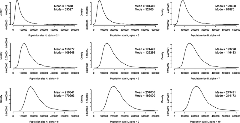
Posterior distributions for the number N of people who inject drugs in St. Petersburg, Russia under different values of α.
We also analyze the St. Petersburg data using the SS-size method described by Handcock, Gile & Mar (2014) and Handcock et al. (2015). Results are shown in Table 1 of the Supplementary Materials. The SS-size model and the method proposed in this paper are quite different, but we have attempted to impose similar prior specifications so that the results are comparable between the two approaches. The posterior estimates from the SS-size method generally fall between 1000 and 4000 when the raw degrees d are used, which is not within the feasible range for the number of PWID in St. Petersburg. Estimates increase to between 20,000 and 100,000 when subjects’ reported degrees are “imputed” by the SS-size software. Estimates under the SS-size model are sensitive to a user-specified maximum N value. Setting this maximum to 500, 000 results in the largest estimates. Aside from the strong influence of the maximum N, the prior distribution imposed on N does not seem to greatly affect the posterior estimates in the SS-size method. Estimates from the SS-size model using the raw degrees d imply that the prevalence of injection drug use is between 0.09% and 0.18% for 20–45 year-olds and between 0.03% and 0.06% for all residents of St. Petersburg, which is far lower than the known minimum prevalence based on the number of registered PWID, and the number of PWID known to be HIV-positive (Heimer & White 2010).
Handcock, Gile & Mar (2014) offer a possible explanation for the performance of the SS-size method for this RDS dataset and population: the SS-size method is thought to work best in larger sample fractions, and gives large interval estimates in small sample fractions. A possible diagnostic test of the SS-size model is suggested by Gile (2011), Handcock, Gile & Mar (2014), Handcock et al. (2015), and Gile et al. (2015), who argue that degrees of subjects recruited by RDS should decrease as the sample accrues. One possible reason for the performance of the SS-size method in this dataset is that the time-ordered degrees do not seem to adhere to this assumption. The mean reported degree in the St. Petersburg dataset is 10.26 with SD 8.5; the maximum reported degree is 200. The Supplementary Materials show the reported degrees and a linear regression line overlaid. To test whether the time-ordered sample of subjects’ degrees decreases, we use the approach suggested by Gile et al. (2015) and regress the integers 1,..., n on the observed degrees d1,... ,dn, ordered by the time of recruitment. We fit several of these regression models using the full dataset of n = 813 reported degrees and with the same dataset excluding one outlier subject who reported degree 200. The results are shown in the Supplementary Materials. The estimated slope coefficient is always small and positive. There does not appear to be a significant negative trend in the reported degrees, and we conclude that there is little evidence that average reported degrees decrease in this dataset.
6. Discussion
We have presented a method for estimating the size of a hidden population from data collected during RDS surveys. The modeling approach relies on several assumptions about the social network connecting members of the target population and the RDS recruitment process. In this section, we examine the basic assumptions underlying the method, and compare them to those made by Handcock, Gile & Mar (2014) and Handcock et al. (2015) in deriving and justifying the SS-size estimator.
We assume that there exists an undirected network G = (V, E) connecting members of the hidden population, and Assumption 2 states that this network follows the Erdős-Rényi distribution. Human social networks are not usually well characterized by the Erdős-Rényi model (Watts & Strogatz 1998, Robins et al. 2001). However, the Erdős-Rényi model has appealing properties in the context of hidden population size estimation: first, the likelihood (2) is simple and does not require calculation of a normalizing constant. Second, the Erdős-Rényi model reflects our general ignorance about the social structure of hidden populations; setting p = 0.5 gives the “uniform” distribution on graphs. Third, because even small subgraphs can provide information about N in the Erdos-Renyi model, (2) does not require that the network be connected, nor that the sample take place in the giant component. Finally, and most importantly, the Erdős-Rényi model has proven to be empirically useful in a wide variety of population size estimation applications via the snowball sampling estimator (Frank & Snijders 1994, Dávid & Snijders 2002) and the network scale-up method (e.g Bernard et al. 2001, Maltiel et al. 2015).
In contrast, the SS-size model of Handcock, Gile & Mar (2014), Handcock et al. (2015) models degrees of unsampled vertices as being drawn independently from a pre-specified parametric distribution. This approach is unburdened by graph-theoretic constraints on the population network, since the set of population degrees drawn in this way need not correspond to the degree sequence of any graph (see e.g. Erdos & Gallai 1960, Tripathi & Vijay 2003). More importantly, inference under the SS-size model is not constrained by topological conditions imposed by the observed recruitment graph GR and the degrees in the subgraph of respondents, as in Definition 5. In the SS-size method, network topology local to recruited vertices does not play a role in recruitment of the sample. This lack of graphical constraints in the SS-size model suggests a view of RDS recruitment that is not network-based: subjects’ reported degrees might be regarded as surrogate measures of “visibility” in the population, and Handcock, Gile & Mar (2014) and Handcock et al. (2015) take sampling probability proportional to visibility.
Assumption 3 states that the probability that a susceptible vertex is recruited depends only on its edges connecting to active recruiters, and does not depend on edges connecting to unsampled vertices. In contrast, the SS-size model of recruitment takes the conditional probability of recruitment to be proportional to the full degree of the potential recruit. The SS-size model also posits that the degrees of recruited subjects should decrease over time as the sample accrues (Johnston et al. 2015, 2016). We did not observe such a decrease in mean degree in the St. Petersburg data (see the Supplementary Materials). Nor did Gile et al. (2015, Supplementary Materials), who find that in robust regression analyses of twelve separate RDS studies, “[s]urprisingly, we find little evidence of decreasing degree over time”. This finding is especially remarkable given that researchers often try to choose high-degree “sociometric stars” as seeds in RDS studies (Wejnert & Heckathorn 2011, page 476).
However, there is reason to believe that network topology matters in determining who can be recruited, that RDS sampling probability is not proportional to degree, and that degrees need not decrease during an RDS study. Crawford (2016) argues that if RDS recruitments happen over edges of a population network, conditional sampling probability has little to do with total degree. Instead, the edges each potential subject (susceptible vertex) shares with recruiters determine their probability of being sampled in the next recruitment. Indeed, a potential subject who shares no edges with recruiters cannot be recruited, regardless of their degree. Worse, sample sizes for RDS studies are usually set in advance, so a potential subject whose shortest path to a seed in G is more than n edges can never be recruited, regardless of their degree. When average degree does not decrease over the time-ordered sample, the assumptions underlying the SS-size method may not be met, and the likelihood of the ordered degrees under the SS-size process may not be informative for N.
We also assume that per-susceptible-edge waiting time to recruitment is memoryless (Assumption 6), which provides a convenient marginalizing distribution over subgraphs in (8). To justify this assumption, we draw an analogy between the RDS recruitment process and the spread of an infectious disease on a population network. The contact process between “susceptible” vertices and “infective” recruiters closely parallels models that have gained wide use in epidemiology. The main difference is that recruiters can deplete their coupons in RDS, which renders them unable to recruit others. The incentive for recruiting other participants in RDS may also provide some justification for exponential waiting times: the need for money may be essentially memoryless. The model of recruitment employed here is drawn largely from Crawford (2016), which provides a detailed study of the sensitivity of subgraph reconstruction to violation of Assumption 6 (exponential waiting times).
All population size estimation methods must make homogeneity assumptions in order to build a probabilistic connection between the sample data and the size of the target population, most of which remains unobserved. In capture-recapture estimation, the homogeneity assumption is random sampling according to a known probability model, usually uniform; in the network scale-up method it is usually that the population graph has Erdős-Rényi distribution; in the SS-size method it is that subjects are drawn with probability proportional to their degree, without replacement. In this paper, we assume that the population network has Erdős-Rényi distribution. The assumptions underlying this method may be justified when researchers believe that the population network exists, is relatively homogeneous, and subjects are recruited across its edges.
RDS was not designed for population size estimation, and it should not be used for this purpose if other options like census enumeration or capture-recapture are available and the assumptions necessary for their use are justified. But RDS remains a popular survey method for good reason: it is a remarkably effective procedure for recruiting subjects who might otherwise be reluctant to participate in a research survey. The lack of better methods for learning about hidden populations suggests to us that RDS will find continued use by epidemiologists and public health researchers in the future. We have shown in this paper that by making some assumptions about the network and the nature of the RDS recruitment process, the observed data from an RDS study can provide useful information about the target population size.
Supplementary Material
Acknowledgements:
FWC was supported by NIH grants NICHD/BD2K DP2HD091799, NIH/NCATS KL2TR000140, NIMH P30MH062294, the Center for Interdisciplinary Research on AIDS, and the Yale Center for Clinical Investigation. We are grateful to Leonid Chindelevitch, Mark Handcock, Edward H. Kaplan, Li Zeng, and three anonymous reviewers for helpful comments. The RDS data presented in the application are from the “Influences on HIV Prevalence and Service Access among IDUs in Russia and Estonia” study, funded by NIH/NIDA grant 1R01DA029888 to Robert Heimer and Anneli Uusküla (Co-PIs). We acknowledge the Yale University Biomedical High Performance Computing Center for computing support, funded by NIH grants RR19895 and RR029676-01.
References
- Abdala N, Carney JM, Durante AJ, Klimov N, Ostrovski D, Somlai AM, Kozlov A & Heimer R (2003), ‘Estimating the prevalence of syringe-borne and sexually transmitted diseases among injection drug users in St Petersburg, Russia’, International Journal of STD & AIDS 14(10), 697–703. [DOI] [PubMed] [Google Scholar]
- Abdul-Quader AS, Baughman AL & Hladik W (2014), ‘Estimating the size of key populations: current status and future possibilities’, Current Opinion in HIV and AIDS 9(2), 107–114. [DOI] [PMC free article] [PubMed] [Google Scholar]
- Balabanova Y, Coker R, Atun R & Drobniewski F (2006), ‘Stigma and HIV infection in Russia’, AIDS Care 18(7), 846–852. [DOI] [PubMed] [Google Scholar]
- Bao L, Raftery AE & Reddy A (2010), Estimating the size of populations at high risk of HIV in Bangladesh using a Bayesian hierarchical model, Technical Report 573, Department of Statistics, University of Washington. [Google Scholar]
- Bao L, Raftery AE & Reddy A (2015), ‘Estimating the sizes of populations at risk of HIV infection from multiple data sources using a Bayesian hierarchical model’, Statistics and Its Interface 8(2), 125. [DOI] [PMC free article] [PubMed] [Google Scholar]
- Berchenko Y & Frost SD (2011), ‘Capture-recapture methods and respondent-driven sampling: their potential and limitations’, Sexually Transmitted Infections 87(4), 267–268. [DOI] [PubMed] [Google Scholar]
- Berchenko Y, Rosenblatt J & Frost SD (2013), ‘Modeling and analysing respondent driven sampling as a counting process’, arXiv preprint arXiv:1304.3505. [DOI] [PubMed] [Google Scholar]
- Bernard HR, Hallett T, Iovita A, Johnsen EC, Lyerla R, McCarty C, Mahy M, Salganik MJ, Saliuk T, Scutelniciuc O et al. (2010), ‘Counting hard-to-count populations: the network scale-up method for public health’, Sexually Transmitted Infections 86(Suppl 2), ii11–ii15. [DOI] [PMC free article] [PubMed] [Google Scholar]
- Bernard HR, Killworth PD, Johnsen EC, Shelley GA & McCarty C (2001), ‘Estimating the ripple effect of a disaster’, Connections 24(2), 18–22. [Google Scholar]
- Bickel PJ, Nair VN & Wang PC (1992), ‘Nonparametric inference under biased sampling from a finite population’, The Annals of Statistics 20, 853–878. [Google Scholar]
- Broadhead RS, Heckathorn DD, Weakliem DL, Anthony DL, Madray H, Mills RJ & Hughes J (1998), ‘Harnessing peer networks as an instrument for AIDS prevention: results from a peer-driven intervention.’, Public Health Reports 113(Suppl 1), 42. [PMC free article] [PubMed] [Google Scholar]
- Burke SE, Calabrese SK, Dovidio JF, Levina OS, Uuskula A, Niccolai LM, Abel-Ollo K & Heimer R (2015), ‘A tale of two cities: Stigma and health outcomes among people with HIV who inject drugs in St. Petersburg, Russia and Kohtla-Jarve, Estonia’, Social Science & Medicine 130, 154–161. [DOI] [PMC free article] [PubMed] [Google Scholar]
- Cepeda JA, Odinokova VA, Heimer R, Grau LE, Lyubimova A, Safiullina L, Levina OS & Niccolai LM (2011), ‘Drug network characteristics and HIV risk among injection drug users in Russia: the roles of trust, size, and stability’, AIDS and Behavior 15, 1003–1010. [DOI] [PMC free article] [PubMed] [Google Scholar]
- Crawford FW (2016), ‘The graphical structure of respondent-driven sampling’, Sociological Methodology 46, 187–211. [DOI] [PMC free article] [PubMed] [Google Scholar]
- David B & Snijders TA (2002), ‘Estimating the size of the homeless population in Budapest, Hungary’, Quality and Quantity 36(3), 291–303. [Google Scholar]
- Draper N & Guttman I (1971), ‘Bayesian estimation of the binomial parameter’, Technometrics 13(3), 667–673. [Google Scholar]
- Erdős P & Gallai T (1960), ‘Gráfok előirt fokszámú pontokkal’, Matematikai Lapok 11, 264–274. [Google Scholar]
- Erdős P & Rényi A (1959), ‘On random graphs’, Publicationes Mathematicae Debrecen 6, 290–297. [Google Scholar]
- Erdős P & Rényi A (1960), ‘On the evolution of random graphs’, Magyar Tud. Akad. Mat. Kutató Int. Közl 5, 17–61. [Google Scholar]
- Ezoe S, Morooka T, Noda T, Sabin ML & Koike S (2012), ‘Population size estimation of men who have sex with men through the network scale-up method in Japan’, Plos One 7(1), e31184. [DOI] [PMC free article] [PubMed] [Google Scholar]
- Feehan DM & Salganik MJ (2016), ‘Generalizing the network scale-up method: A new estimator for the size of hidden populations’, Sociological Methodology 46(1), 153–186. [DOI] [PMC free article] [PubMed] [Google Scholar]
- Feehan DM, Umubyeyi A, Mahy M, Hladik W & Salganik MJ (2016), ‘Quantity versus quality: A survey experiment to improve the network scale-up method’, American Journal of Epidemiology 183(8), 747–757. [DOI] [PMC free article] [PubMed] [Google Scholar]
- Félix-Medina MH & Monjardin PE (2009), ‘Link-tracing sampling with an initial sequential sample of sites: Estimating the size of a hidden human population’, Statistical Methodology 6(5), 490–502. [Google Scholar]
- Félix-Medina MH & Thompson SK (2004), ‘Combining link-tracing sampling and cluster sampling to estimate the size of hidden populations’, Journal of Official Statistics 20(1), 19–38. [Google Scholar]
- Fienberg SE (1972), ‘The multiple recapture census for closed populations and incomplete 2k contingency tables’, Biometrika 59(3), 591–603. [Google Scholar]
- Frank O & Snijders T (1994), ‘Estimating the size of hidden populations using snowball sampling’, Journal of Official Statistics 10, 53–53. [Google Scholar]
- Gile KJ (2011), ‘Improved inference for respondent-driven sampling data with application to HIV prevalence estimation’, Journal of the American Statistical Association 106(493), 135–146. [Google Scholar]
- Gile KJ & Handcock MS (2010), ‘Respondent-driven sampling: An assessment of current methodology’, Sociological Methodology 40(1), 285–327. [DOI] [PMC free article] [PubMed] [Google Scholar]
- Gile KJ, Johnston LG & Salganik MJ (2015), ‘Diagnostics for respondent-driven sampling’, Journal of the Royal Statistical Society A 178, 241–269. [DOI] [PMC free article] [PubMed] [Google Scholar]
- Goodman LA (1961), ‘Snowball sampling’, The Annals of Mathematical Statistics 32(1), 148–170. [Google Scholar]
- Guo W, Bao S, Lin W, Wu G, Zhang W, Hladik W, Abdul-Quader A, Bulterys M, Fuller S & Wang L (2013), ‘Estimating the size of HIV key affected populations in Chongqing, China, using the network scale-up method’, PloS One 8(8), e71796. [DOI] [PMC free article] [PubMed] [Google Scholar]
- Habecker P, Dombrowski K & Khan B (2015), ‘Improving the network scale-up estimator: Incorporating means of sums, recursive back estimation, and sampling weights’, PloS one 10(12). [DOI] [PMC free article] [PubMed] [Google Scholar]
- Hall WD, Ross JE, Lynskey MT, Law MG & Degenhardt LJ (2000), ‘How many dependent heroin users are there in Australia?’, Medical Journal of Australia 173(10), 528–531. [DOI] [PubMed] [Google Scholar]
- Handcock MS, Fellows IE & Gile KJ (2014), RDS Analyst: Software for the Analysis of Respondent-Driven Sampling Data, Los Angeles, CA. Version 0.42. URL: http://hpmrg.org
- Handcock MS, Gile KJ & Mar CM (2014), ‘Estimating hidden population size using respondent-driven sampling data’, Electronic Journal of Statistics 8(1), 1491–1521. [DOI] [PMC free article] [PubMed] [Google Scholar]
- Handcock MS, Gile KJ & Mar CM (2015), ‘Estimating the size of populations at high risk for hiv using respondent-driven sampling data’, Biometrics 71(1), 258–266. [DOI] [PMC free article] [PubMed] [Google Scholar]
- Heckathorn DD (1997), ‘Respondent-driven sampling: a new approach to the study of hidden populations’, Social Problems 44(2), 174–199. [Google Scholar]
- Heimer R & White E (2010), ‘Estimation of the number of injection drug users in St. Petersburg, Russia’, Drug and Alcohol Dependence 109(1), 79–83. [DOI] [PMC free article] [PubMed] [Google Scholar]
- Hickman M, Hickman M, Hope V, Platt L, Higgins V, Bellis M, Rhodes T, Taylor C & Tilling K (2006), ‘Estimating prevalence of injecting drug use: a comparison of multiplier and capture-recapture methods in cities in England and Russia’, Drug and Alcohol Review 25(2), 131–140. [DOI] [PubMed] [Google Scholar]
- Hunter DR & Handcock MS (2006), ‘Inference in curved exponential family models for networks’, Journal of Computational and Graphical Statistics 15(3), 565–583. [Google Scholar]
- Johnston LG, McLaughlin KR, El Rhilani H, Latifi A, Toufik A, Bennani A, Alami K, Elomari B & Handcock MS (2015), ‘Estimating the size of hidden populations using respondent-driven sampling data: Case examples from Morocco’, Epidemiology 26(6), 846–852. [DOI] [PMC free article] [PubMed] [Google Scholar]
- Johnston LG, McLaughlin KR, Rouhani SA & Bartels SA (2016), ‘Measuring a hidden population: A novel technique to estimate the population size of women with sexual violence-related pregnancies in South Kivu Province, Democratic Republic of Congo’, Journal of Epidemiology and Global Health In Press,−. [DOI] [PMC free article] [PubMed] [Google Scholar]
- Kadushin C, Killworth PD, Bernard HR & Beveridge AA (2006), ‘Scale-up methods as applied to estimates of heroin use’, Journal of Drug Issues 36(2), 417–440. [Google Scholar]
- Kahn WD (1987), ‘A cautionary note for Bayesian estimation of the binomial parameter n’, The American Statistician 41(1), 38–40. [Google Scholar]
- Kaplan EH & Soloshatz D (1993), ‘How many drug injectors are there in New Haven? Answers from AIDS data’, Mathematical and Computer Modelling 17(2), 109–115. [Google Scholar]
- Khalid FJ, Hamad FM, Othman AA, Khatib AM, Mohamed S, Ali AK & Dahoma MJ (2014), ‘Estimating the number of people who inject drugs, female sex workers, and men who have sex with men, Unguja Island, Zanzibar: results and synthesis of multiple methods’, AIDS and Behavior 18(1), 25–31. [DOI] [PubMed] [Google Scholar]
- Killworth PD, McCarty C, Bernard HR, Shelley GA & Johnsen EC (1998), ‘Estimation of seroprevalence, rape, and homelessness in the United States using a social network approach’, Evaluation Review 22(2), 289–308. [DOI] [PubMed] [Google Scholar]
- Kozlov AP, Shaboltas AV, Toussova OV, Verevochkin SV, Masse BR, Perdue T, Beauchamp G, Sheldon W, Miller WC, Heimer R et al. (2006), ‘HIV incidence and factors associated with HIV acquisition among injection drug users in St Petersburg, Russia’, AIDS 20(6), 901–906. [DOI] [PubMed] [Google Scholar]
- Larson A, Stevens A & Wardlaw G (1994), ‘Indirect estimates of ‘hidden’ populations: capture-recapture methods to estimate the numbers of heroin users in the Australian Capital Territory’, Social Science & Medicine 39(6), 823–831. [DOI] [PubMed] [Google Scholar]
- Laska EM, Meisner M & Siegel C (1988), ‘Estimating the size of a population from a single sample’, Biometrics pp. 461–472. [PubMed] [Google Scholar]
- Malmros J, Liljeros F & Britton T (2014), ‘Respondent-driven sampling and an unusual epidemic’, arXiv preprint arXiv:1411.4867. [Google Scholar]
- Maltiel R, Raftery AE, McCormick TH & Baraff AJ (2015), ‘Estimating population size using the network scale up method’, The Annals of Applied Statistics 9(3), 1247–1277. [DOI] [PMC free article] [PubMed] [Google Scholar]
- McCormick TH, Salganik MJ & Zheng T (2010), ‘How many people do you know?: Efficiently estimating personal network size’, Journal of the American Statistical Association 105(489), 59–70. [DOI] [PMC free article] [PubMed] [Google Scholar]
- Niccolai LM, Toussova OV, Verevochkin SV, Barbour R, Heimer R & Kozlov AP (2010), ‘High HIV prevalence, suboptimal HIV testing, and low knowledge of HIV-positive serostatus among injection drug users in St. Petersburg, Russia’, AIDS and Behavior 14, 932–941. [DOI] [PMC free article] [PubMed] [Google Scholar]
- Niccolai LM, Verevochkin SV, Toussova OV, White E, Barbour R, Kozlov AP & Heimer R (2011), ‘Estimates of HIV incidence among drug users in St. Petersburg, Russia: continued growth of a rapidly expanding epidemic’, The European Journal of Public Health 21, 613–619. [DOI] [PMC free article] [PubMed] [Google Scholar]
- Nikfarjam A, Shokoohi M, Shahesmaeili A, Haghdoost AA, Baneshi MR, Haji-Maghsoudi S, Rastegari A, Nasehi AA, Memarian N & Tarjoman T (2016), ‘National population size estimation of illicit drug users through the network scale-up method in 2013 in Iran’, International Journal of Drug Policy. [DOI] [PubMed] [Google Scholar]
- Paz-Bailey G, Jacobson J, Guardado M, Hernandez F, Nieto A, Estrada M & Creswell J (2011), ‘How many men who have sex with men and female sex workers live in El Salvador? using respondent-driven sampling and capture-recapture to estimate population sizes’, Sexually transmitted infections 87(4), 279–282. [DOI] [PubMed] [Google Scholar]
- Pokrovsky V, Ladnaya N & Buravtsova E (2010), ‘HIV infection: Information bulletin # 34’, Moscow, RF: Russian Federal AIDS Center. [Google Scholar]
- Quaye S, Raymond HF, Atuahene K, Amenyah R, Aberle-Grasse J, McFarland W, El-Adas A, Group GMS et al. (2015), ‘Critique and lessons learned from using multiple methods to estimate population size of men who have sex with men in Ghana’, AIDS and Behavior 19(1), 16–23. [DOI] [PubMed] [Google Scholar]
- Raftery AE (1988), ‘Inference for the binomial N parameter: A hierarchical Bayes approach’, Biometrika 75(2), 223–228. [Google Scholar]
- Rhodes T, Sarang A, Bobrik A, Bobkov E & Platt L (2004), ‘HIV transmission and HIV prevention associated with injecting drug use in the Russian Federation’, International Journal of Drug Policy 15(1), 1–16. [Google Scholar]
- Robins G, Elliott P & Pattison P (2001), ‘Network models for social selection processes’, Social Networks 23(1), 1–30. [Google Scholar]
- Sabin K, Zhao J, Calleja JMG, Sheng Y, Garcia SA, Reinisch A & Komatsu R (2016), ‘Availability and quality of size estimations of female sex workers, men who have sex with men, people who inject drugs and transgender women in low-and middle-income countries’, PloS one 11(5), e0155150. [DOI] [PMC free article] [PubMed] [Google Scholar]
- Salganik MJ, Fazito D, Bertoni N, Abdo AH, Mello MB & Bastos FI (2011), ‘Assessing network scale-up estimates for groups most at risk of HIV/AIDS: evidence from a multiple-method study of heavy drug users in Curitiba, Brazil’, American Journal of Epidemiology 174(10), 1190–1196. [DOI] [PMC free article] [PubMed] [Google Scholar]
- Salganik MJ & Heckathorn DD (2004), ‘Sampling and estimation in hidden populations using respondent-driven sampling’, Sociological Methodology 34(1), 193–240. [Google Scholar]
- Sarang A, Rhodes T & Sheon N (2012), ‘Systemic barriers accessing HIV treatment among people who inject drugs in Russia: a qualitative study’, Health policy and planning p. czs107. [DOI] [PMC free article] [PubMed] [Google Scholar]
- Shaboltas AV, Toussova OV, Hoffman IF, Heimer R, Verevochkin SV, Ryder RW, Khoshnood K, Perdue T, Masse BR & Kozlov AP (2006), ‘HIV prevalence, sociodemographic, and behavioral correlates and recruitment methods among injection drug users in St. Petersburg, Russia’, Journal of Acquired Immune Deficiency Syndromes 41(5), 657–663. [DOI] [PubMed] [Google Scholar]
- Shelley GA, Bernard HR, Killworth P, Johnsen E & McCarty C (1995), ‘Who knows your HIV status? What HIV+ patients and their network members know about each other’, Social Networks 17(3), 189–217. [Google Scholar]
- Shelley GA, Killworth PD, Bernard HR, McCarty C, Johnsen EC & Rice RE (2006), ‘Who knows your HIV status II?: Information propagation within social networks of seropositive people’, Human Organization 65(4), 430–444. [Google Scholar]
- Shelton JF (2015), ‘Proposed utilization of the network scale-up method to estimate the prevalence of trafficked persons’, Forum on Crime and Society: Special issue Researching hidden populations: approaches to and methodologies for generating data on trafficking in persons 8, 85–94. [Google Scholar]
- Shokoohi M, Baneshi MR & Haghdoost A (2012), ‘Size estimation of groups at high risk of HIV/AIDS using network scale up in Kerman, Iran’, International Journal of Preventive Medicine 3(7), 471. [PMC free article] [PubMed] [Google Scholar]
- Snidero S, Corradetti R & Gregori D (2004), ‘The network scale-up method: A simulation study in case of overlapping sub-populations’, Metodoloski Zvezki 1(2), 395–405. [Google Scholar]
- Thein ST, Aung T & McFarland W (2015), ‘Estimation of the number of female sex workers in Yangon and Mandalay, Myanmar’, AIDS and Behavior 19(10), 1941–1947. [DOI] [PubMed] [Google Scholar]
- Thompson SK (2006), ‘Adaptive web sampling’, Biometrics 62(4), 1224–1234. [DOI] [PubMed] [Google Scholar]
- Tripathi A & Vijay S (2003), ‘A note on a theorem of Erdos & Gallai’, Discrete Mathematics 265(1), 417–420. [Google Scholar]
- UNAIDS (2010a), ‘Global report: UNAIDS report on the global AIDS epidemic 2010’, UNAIDS Geneva. URL: http://www.unaids.org/globalreport/
- UNAIDS (2010b), Guidelines on Estimating the Size of Populations Most at Risk to HIV, UNAIDS/WHO Working Group on Global HIV/AIDS and STI Surveillance, Geneva, Switzerland. [Google Scholar]
- van der Heijden PG, de Vries L, Bohning D & Cruyff M (2015), ‘Estimating the size of hard-to-reach populations using capture-recapture methodology, with a discussion of the International Labour Organization’s global estimate of forced labour’, Forum on Crime and Society: Special issue Researching hidden populations: approaches to and methodologies for generating data on trafficking in persons 8, 109–136. [Google Scholar]
- Vincent K & Thompson S (2012), ‘Estimating population size with link-tracing sampling’, arXiv preprint arXiv:1210.2667. [Google Scholar]
- Volz E & Heckathorn DD (2008), ‘Probability based estimation theory for respondent driven sampling’, Journal of Official Statistics 24(1), 79–97. [Google Scholar]
- Wang J, Yang Y, Zhao W, Su H, Zhao Y, Chen Y, Zhang T & Zhang T (2015), ‘Application of network scale up method in the estimation of population size for men who have sex with men in shanghai, china’, PLoS ONE 10(11), 1–12. [DOI] [PMC free article] [PubMed] [Google Scholar]
- Watts DJ & Strogatz SH (1998), ‘Collective dynamics of ‘small-world’ networks’, Nature 393(6684), 440–442. [DOI] [PubMed] [Google Scholar]
- Wejnert C & Heckathorn D (2011), Respondent-driven sampling: operational procedures, evolution of estimators, and topics for future research, in Williams M & Vogt WP, eds, ‘The SAGE handbook of innovation in social research methods. London: SAGE Publications, Ltd’, SAGE Publications, Inc; Thousand Oaks, CA, pp. 473–97. [Google Scholar]
- Wesson P, Handcock MS, McFarland W & Raymond HF (2015), ‘If you are not counted, you don’t count: Estimating the number of african-american men who have sex with men in san francisco using a novel bayesian approach’, Journal of Urban Health 92(6), 1052–1064. [DOI] [PMC free article] [PubMed] [Google Scholar]
- World Health Organization (2005), ‘Russian Federation: Summary country profile for HIV/AIDS treatment scale-up’. URL: http://www.who.int/hiv/HIVCP-RUS.pdf
- World Health Organization (2014), ‘Consolidated guidelines on HIV prevention, diagnosis, treatment and care for key population’. URL: http://who.int/hiv/pub/guidelines/keypopulations/en/ [PubMed]
- Zheng T, Salganik MJ & Gelman A (2006), ‘How many people do you know in prison? Using overdispersion in count data to estimate social structure in networks’, Journal of the American Statistical Association 101(474), 409–423. [Google Scholar]
Associated Data
This section collects any data citations, data availability statements, or supplementary materials included in this article.