PyMINEr Finds Gene and Autocrine-Paracrine Networks from Human Islet scRNA-Seq

SUMMARY

Toolsets available for in-depth analysis of scRNA-seq datasets by biologists with little informatics experience is limited. Here, we describe an informatics tool (PyMINEr) that fully automates cell type identification, cell type-specific pathway analyses, graph theory-based analysis of gene regulation, and detection of autocrine-paracrine signaling networks in silico. We applied PyMINEr to interrogate human pancreatic islet scRNA-seq datasets and discovered several features of co-expression graphs, including concordance of scRNA-seq-graph structure with both protein-protein interactions and 3D genomic architecture, association of high-connectivity and low-expression genes with cell type enrichment, and potential for the graph structure to clarify potential etiologies of enigmatic disease-associated variants. We further created a consensus co-expression network and autocrine-paracrine signaling networks within and across islet cell types from seven datasets. PyMINEr correctly identified changes in BMP-WNT signaling associated with cystic fibrosis pancreatic acinar cell loss. This proof-of-principle study demonstrates that the PyMINEr framework will be a valuable resource for scRNA-seq analyses.

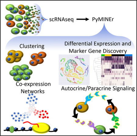
Graphical Abstract

In Brief

Tyler et al. create PyMINEr, an open-source program (https://www.sciencescott.com/pyminer) that automates analyses of expression datasets without coding. These analyses include clustering, differential expression, pathway analyses, co-expression networks, marker gene identification, and autocrine-paracrine signaling prediction. Integration of seven datasets shows elevated BMP-WNT signaling in cystic fibrosis pancreata.

INTRODUCTION

Recent advances in single-cell RNA sequencing (scRNA-seq) provide a rich resource of omic-level data that can help dissect the complex signaling networks that govern cellular identity and function (Jaitin et al., 2016; Patel et al., 2014). scRNA-seq presents a cornucopia of data to bench scientists; however, for those accustomed to more traditional datasets, the overwhelming informatics tasks at hand can be daunting. To streamline the transition from the 2D matrix of scRNA-seq data into meaningful biologic insights, we created a tool called Python Maximal Information Network Exploration Resource (PyMINEr), which addresses the gaps described below.

The first task when analyzing scRNA-seq data is identification of cell types. Cell type identification is often performed by clustering on a subset of genes, similarity or distance measures, or an otherwise dimensionally reduced version of the transcriptome. The next step often performed is iterative traditional k-means clustering of the selected features (Grün et al., 2015; Kiselev et al., 2017; Shin et al., 2015); however, previous research showed that the traditional k-means clustering approach yields highly variable results (Arthur and Vassilvitskii, 2007). Another pitfall of k-means clustering is the requirement for the user to specify the number of groups (in the case of scRNA-seq, the number of cell types), necessitating more unbiased methods for determining the number of cell types (Grün et al., 2015). This a priori specification will bias the outcome of clustering and, thus, data interpretation. Overall, the methods of analysis following cell type identification can also be quite variable.

Social network-style graph networks have been used previously to analyze RNA-seq data, with nodes in the graph representing genes, and a direct connection between two genes indicating that they are co-expressed (Hong et al., 2013; Iancu et al., 2012; Langfelder and Horvath, 2008); however, co-expression graphs are often underutilized when interrogating these datasets. Because gene expression patterns underlie the structure of expression graphs, this structure can be used to study transcriptional features of cellular identity in normal and pathologic disease states. By way of analogy, social network connectivity between individuals can reveal important information about the friends and behaviors of individuals; we integrate this within our automated pipeline, applied to gene expression.

Aberrant gene regulation underlies many aspects of human diseases; dysfunction of pancreatic endocrine and exocrine cells in diabetes is one well-recognized example (Porte, 1991). Pancreatic disease can manifest as aberrant hormone processing and secretion, dysregulated autocrine or paracrine signaling, changes to cell identity, and/or alterations in transcriptional control of these processes (Grant et al., 2006; Khodabandehloo et al., 2016; Nicolson et al., 2009; Prentki and Nolan, 2006; Rutter et al., 2015). Insights into genes that may affect the development of type 2 diabetes (T2D) have emerged from genome-wide analysis of associated SNPs; however, the functional significance of many coding and non-coding SNPs remains obscure (Morris et al., 2012). Given the systems-level complexity of diabetes, we selected this disease to leverage the power of the PyMINEr analytic pipeline with human islet scRNA-seq.

A cell’s local environment affects numerous processes that define its identity and function in both health and disease. In fact, many cell fate decisions are made in response to extracellular input provided by secreted cytokines interacting with their receptors (Behfar et al., 2002; Gnecchi et al., 2008; Watabe and Miyazono, 2009). Transcripts that encode secreted ligands and their cognate receptors are embedded in scRNA-seq data-sets, suggesting that scRNA-seq alone may be sufficient to reveal a cell’s ability to signal to itself and to other cells. However, it is not yet possible to automatically convert this information to knowledge of cell type-specific autocrine and paracrine signaling.

To address the above described gaps, we created PyMINEr. This tool enables analysis of scRNA-seq data by integrating expression graphs with information about protein-protein interactions (Szklarczyk et al., 2015), cell type enrichment, SNP genome-wide associations (Morris et al., 2012), and protein:DNA interactions (chromatin immunoprecipitation sequencing [ChIP-seq]) (ENCODE Project Consortium, 2012), all in a fully integrated pipeline that performs each of these tasks with little effort by the user. We demonstrate that co-expression graphs harbor many relationships that are latent and typically unseen but biologically important. In addition, we have integrated PyMINEr analyses of 7 different human scRNA-seq datasets (7,603 cells), creating a consensus co-expression network and autocrine-paracrine signaling network. Our examination of the autocrine-paracrine circuits within and between islet cell types identified by PyMINEr correctly predicted that the pancreatic acinar cell ablation seen in human cystic fibrosis (CF) pancreata would lead to the induction of the BMP and WNT pathways. Rather than providing a library of functions that are individually applied programmatically, nearly all of the informatic tasks described here are performed by PyMINEr with a single command line that generates a hypertext markup language (html) web display explanation of the results. PyMINEr can be applied to any dataset to uncover the structure underlying the corresponding complex biologic systems.

RESULTS

PyMINEr Overview

To address the informatic challenges presented by scRNA-seq, we sought to produce a tool that rapidly translates an unlabeled 2D expression matrix to biologically interpretable and actionable hypotheses. The challenges addressed by PyMINEr include automated cell type identification, basic statistics comparing cell types with each other, pathway analyses of the genes enriched in each cell type, and the generation of co-expression networks that enable a graph theory approach to interpreting gene expression. Last, we integrated an approach for predicting autocrine-paracrine signaling networks in silico and pathway analyses that enable a deeper understanding of the signaling networks between cells. These informatic analyses are performed with a single short command line that generates an html web page of the collated PyMINEr results (Figure 1A). An example of the output generated by PyMINEr is provided in the tutorials (https://www.sciencescott.com/pyminer). All methods and algorithms are described in detail in the STAR Methods. Below, we describe scRNA-seq of human pancreatic islets and application of the PyMINEr analytic pipeline as a test case (Figure 1B).

Figure 1. PyMINEr Pipeline and Implementation for scRNA-Seq.

(A) An example command line input for running PyMINEr, for which the only required argument is the input file. If you have genes of interest however, this can also be provided. At the end of a PyMINEr run, an interactive html file organizing and describing the results is generated.

(B) The PyMINEr analytic pipeline as utilized in this study. We used PyMINEr to analyze scRNA-seq, identify cell types, and generate expression graph networks integrated with Z score enrichment for each cell type. Integration of the graph structure and cell type enrichment analyses with GWAS data enabled the identification of several previously undescribed cell type-specific expression patterns for poorly described type 2 diabetes (T2D)-associated genes. The automated generation of autocrine and paracrine signaling networks through PyMINEr enabled confirmation of hypotheses predicted for the diseased human cystic fibrosis pancreas, where cellular compartments are remodeled.

See STAR Methods and Figures S1–S3 for details regarding clustering methods and benchmarking.

Cell Type Identification Using PyMINEr

The problem of clustering cells into their appropriate cell types has two components: (1) identifying cells that are sufficiently similar to each other to be considered members of the same cell type, and (2) establishing the number of cell types present in the dataset. For the identification of similar cells, we devised an algorithm using an “anti-gravity” style method of centroid seeding for k-means clustering (Figure S1; see STAR Methods for details). For synthetic (Figures S2A and S2B) and real-world (Figures S2C–S2G) datasets, this method of clustering was more accurate than either the traditional k-means or k-means++ methods, as measured by cluster purity, entropy, or mutual information. We also developed an algorithm to determine the number of cell types in the dataset (Figures S3A–S3F). It was more accurate than the maximum gap statistic, a previously published method implemented in RaceID (a previously published software for identifying cell types from scRNA-seq) (Figures S3G–S3I; Grün et al., 2015). Indeed, PyMINEr showed a greater level of self-consistency compared with RaceID with respect to identifying cell types from scRNA-seq data (Figures S3I–S3M).

Application of the PyMINEr analytic pipeline to our human pancreatic islet scRNA-seq dataset revealed eight major cell types within human islets, including endocrine cells (beta, alpha, epsilon, delta, and pancreatic polypeptide cells), exocrine cells (acinar and ductal cells), and stromal cells. PyMINEr-based identification of cell types and categorization of differentially expressed genes between cell types (Figures 2A–2C; Tables S1 and S2) led to the rediscovery of many known but also the discovery of unknown islet cell type-enriched genes. PyMINEr automates pathway analysis of the gene lists associated with each cell type (Tables S2C–S2E). Notably, PyMINEr’s entropy-based pathway meta-analyses correctly identified beta cells as endocrine pancreatic cells (HPA:031020) through integrated gProfiler Human Protein Atlas (HPA) analyses (Reimand et al., 2016; Uhlén et al., 2015). Similarly, PyMINEr correctly identified acinar cells as the most abundant pancreatic exocrine cell type (HPA:031010) (Figure 2B; Tables S2D and S2E). These findings demonstrate that the pathway analyses integrated in PyMINEr can correctly identify the tissue of origin from scRNA-seq data. See STAR Methods for details regarding pathway analyses.

Figure 2. Characterization of Human Pancreatic Islet scRNA-Seq Gene Enrichment and Network Graphs.

(A) A heatmap of each cell type and an associated cell type marker. Cell types are color-coded along the top of the heatmap, with colors matching those in (C).

(B) The top five Human Protein Atlas (HPA) pathways for beta cells (top, red) and acinar cells (bottom, brown). Importantly, integrated pathway analyses by PyMINEr correctly identified the human body part and sub-organ.

(C) The number of genes enriched in each identified cell type as identified by PyMINEr.

(D) Examples of expression relationships that give rise to the network model of transcription based on scRNA-seq data. Cell type-enriched genes (INS and MAFA in beta cells, CELA3A and AMY2A in acinar cells) are co-expressed in particular cell types. Points in the scatterplots correspond to the expression level of the indicated gene; the identity of the associated cell is indicated by the color of the point. Of particular note are beta cells (red) and acinar cells (brown); other cell types are color-coded as in (C). Black lines show locally estimated scatterplot smoothing (LOESS) of locally weighted regressions. Spearman correlation rho and p values are shown for gene-gene expression relationships for cell type-enriched genes.

(E) Graphic representation of cell type Z score enrichment, illustrating differences in transcriptional networks across cell types. For most cell types, certain regions within the network showed transcriptional enrichment across the topology of the network.

PyMINEr Co-expression Graphs

Representing RNA-seq data as a social network-style graph (via expression correlations) has several advantages. Graph networks make it possible to use graph theory analyses, which are not frequently used in basic biology. PyMINEr identifies all non-parametric Spearman correlations between genes, creating a graph network in which a connection between two genes indicates that their expression is correlated; in other words, the genes are co-expressed. Because of the non-linear relationships associated with transcription at the cellular level (Levine et al., 2013), this approach is better suited than parametric methods (Hong et al., 2013; Iancu et al., 2012; Langfelder and Horvath, 2008) for discovering transcriptional relationships in the context of scRNA-seq. As expected, PyMINEr revealed strong correlations between genes that are enriched within the same cell type; these correlations are represented as direct connections within the network (Table S2F; Figure 2D). In fact, when the network was overlaid with gene enrichment Z scores for each cell type, domains of high expression enrichment were observed for each islet cell type (Figure 2E).

Graph Networks Are Reproducible from scRNA-Seq across Platforms

Recently, the scRNA-seq field has begun to favor datasets with more cells sequenced at lower depth rather than datasets with few cells sequenced deeply. To test whether the co-expression networks built by PyMINEr are robust to the trade-off of cell number and sequencing depth, we compared network topologies built from our human islet scRNA-seq dataset (few cells at high depth) to one produced by others (more cells at low depth) (Table S3; Segerstolpe et al., 2016). Consistent with the expectation that PyMINEr is robust in both scenarios, the overall graph structures created by PyMINEr for each of the two datasets were highly concordant (Spearman rho = 0.36, p ≈ 0.0; Pearson R = 0.32, p ≈ 0.0; χ² = 868,755, p ≈ 0.0; Figures 3A and 3B; Tables S2F and S3C).

Figure 3. Graph Structure Is Conserved across Human Islet scRNA-Seq Datasets from Different Laboratories.

(A) A schematic example of the shortest path between two genes in a network. In this case, the shortest path between gene A and gene B is two, denoted by the red lines (i.e., A and B are 2 degrees of separation away from each other).

(B) The correlation corresponding to overall network structure when comparing the network built by PyMINEr using our dataset and the dataset from Segerstolpe et al. (2016). The plot indicates the shortest path between all gene-gene pairs within each network. Linear regression is shown by the blue line. These results indicate that the overall structures of the two networks built by these two datasets are similar. Of note, our dataset contained fewer cells (185) sequenced at a higher depth (average reads per cell = 2,842,414; i.e., 1,421,207 paired-end fragments). This demonstrates that, with sufficient depth of sequence, network graphs can be generated with fewer cells.

(C) Heatmaps of known and posited islet marker genes form the 6 additional datasets analyzed here. Full PyMINEr analyses for these datasets available at www.sciencescott.com/pancreatic-scrnaseq. See Figure S4 for notes regarding adjusting for variable power across datasets for constructing graph networks.

To provide a broadly useful resource to the fields of pancreatic biology, we analyzed 6 additional datasets (7 including our own), amassing a resource created from 7,603 human islet cells (Figure 3C; Li et al., 2016; Muraro et al., 2016; Segerstolpe et al., 2016; Wang et al., 2016; Xin et al., 2016). Using these analyses, we also created a consensus expression network of gene-gene correlations found in 33% or more of datasets (analyses available at https://www.sciencescott.com/ pancreatic-scrnaseq). We also examined these datasets for the expression of newly proposed beta cell marker genes, including markers of mature beta cells (flattop:FLTP [Bader et al., 2016]; urocortin3:UCN3 [van der Meulen et al., 2012]). In contrast to what is observed in the intact pancreas, these genes were expressed in very few islet cells (Bader et al., 2016; van der Meulen et al., 2012), suggesting loss of mature beta cells in cultured human pancreatic islets. Others have proposed four unique subsets of beta cells with variable positivity for CD9 and ST8AI1. Although we observed relatively similar proportions of these beta cells, as reported previously (Dorrell et al., 2016), we also observed expression of these genes in many different endocrine and non-endocrine cells (Figure 3C); this may indicate that these genes are representative of a cell state as opposed to a cell type. Lineage trace experiments in animal models will likely be needed to determine the stability of these newly proposed marker genes.

Expression Graph Networks Are Enriched for Physical Protein-Protein Interactions and Genomic Neighborhoods

Given the premise that genes whose protein products function together at the molecular level must be co-expressed within the same cell (Figure 4A), we hypothesized that co-expressed genes (i.e., first neighbors or one-degree separated genes) are likely to physically interact with each other. To test this hypothesis, we compared the transcriptional graph network defined by PyMINEr with previously annotated protein-protein interactions (Szklarczyk et al., 2015). Indeed, protein-protein interactions were over-represented in the PyMINEr-generated network (10.9-fold increase over random; one-sample t test: p = 4.7e −23; n = 10 Monte Carlo simulations) (Figure 4B). This outcome suggests that previously undescribed interactions may be represented in the expression graph and further indicates that genes involved in related cellular processes have evolved to maintain coordinated transcription.

Figure 4. Graph Structure Is Related to Protein-Protein Interactions and CTCF-Cohesin Demarcations in the Genome.

(A) Schematic illustration of the rationale for the experiment. Given that the two physically interacting proteins must be present within the same cell, it follows that the transcripts of these genes might be co-regulated.

(B) Among co-regulated genes, the percentage of those known to interact (based on StringDB) is significantly higher than those in simulated random networks derived from a Monte Carlo random pairing of expressed genes to create equally long adjacency lists (p = 4.73e–23, n = 10 simulations, 2-sided 1-sample t test). This indicates that the co-regulatory network generated by PyMINEr can yield biologically meaningful results.

(C) Log10 distances between the RAD21, CTCF, and SMC3 binding sites from each other. Each plane corresponds to the binding sites for the indicated transcription factor; the distance of that binding site from its nearest binding site for the other two factors is then noted in the scatterplot. Red points are positive for RAD21, CTCF, and SMC3, all within 150 bases of each other. Blue points represent loci that are bound by RAD21 and CTCF within 150 bases, but the nearest SMC3 binding site was over 150 bases away. Red and blue populations were used as insulator demarcations across the genome.

(D) A schematic illustration of insulating CTCF-cohesin loci, which partition the genome into insulated domains.

(E) We observed significant concordance between the co-expression graph from scRNA-seq and the graph representing the genes partitioned between n insulation sites (x axis). Interestingly, we also observed a modest enrichment for gene co-expression in gene-gene pairs separated by one or two insulating sites; however, this significance disappears in gene-gene pairs separated by three or four insulating sites. This evidence fits with the model of genome conformation manifest from CTCF-cohesin loop extrusion with optional stopping sites. This observation also indicates that, although the regulatory elements within a single insulated domain are strongest, there remains regulatory bleedover across insulation sites, likely because of stochastic CTCF binding site skipping during the process of loop extrusion (Sanborn et al., 2015).

See Figure S5 and Table S4 for other notable properties of the graph structure as it pertains to cell type-specific gene expression patterns.

We also hypothesized that coordinated transcription between insulator sites would be detectable using the PyMINEr-generated co-expression graph. To test this hypothesis, we examined concordance between the structure of PyMINEr co-expression graph and a graph network generated by connecting all genes located between two adjacent CCCTC-binding factor (CTCF)/cohesin insulator sites. Indeed, genes located between the same insulator sites were more likely than expected by chance to share a direct network connection in the graph structure generated from human islet scRNA-seq (χ² = 596.2, p = 1.12e−131; Figures 4C–4E). Thus, the transcription graph structure is directly related to the binding loci of the insulating CTCF-cohesin complexes that orchestrate the 3D conformation of the genome.

Empirical Power Adjustment for Network Construction without Imputation

Variable levels of dropout in scRNA-seq result in variable power for detecting gene-gene correlations when constructing networks. Several methods have recently been developed to impute these missing values to prevent this change in power. We benchmarked two of these methods, SAVER (Huang et al., 2018) and scImpute (Li and Li, 2018), assessing their effect on network structure. Both methods caused large-scale structural changes to the network built from our scRNA-seq dataset (Figure S4A; networks built from Table S1A or imputed versions of it); SAVER tended to blur relationships into a single co-regulated gene set (Figures S4A and S4B), whereas scImpute drastically altered structure in a manner directly attributable to the manually set hyperparameter determining the number of cell types (Figure S4A). Given these results, we hypothesized that scImpute would synthesize the number of clusters a user requests even from completely random data. Indeed, when fed a synthetic random dataset, scImpute created clearly separable clusters in the exact number specified by the user (Figure S4C). To our knowledge, all imputation methods violate the assumption of independence of measures, decreasing within group variance, and increasing between group variance. Although imputed datasets may be appropriate for some forms of analyses, the violation of this assumption makes imputed datasets less appropriate for statistical comparison between cell types.

Because of these imputation issues, we implemented an empirical false positive measure to determine the appropriate Spearman correlation cutoff in creating a graph network. This dynamic cutoff algorithm performs bootstrap shuffling on the dataset to determine the null distribution of Spearman correlations when no true relationships exist. This enables PyMINEr to build expression networks with an automatic power adjustment without altering the original dataset or violating the assumptions of independence required by all statistical tests.

Last, an issue with creating co-expression networks lies in the large scale of the computation problem. Every gene must be compared with all other genes, thus requiring 2.65e8 comparisons. Furthermore, the size of scRNA-seq datasets are growing at an exceptional rate; we therefore benchmarked PyMINEr’s correlation algorithm to EGAD’s, a recently released R package created for this purpose. We found that PyMINEr’s network construction implementation is substantially and significantly faster (25- to 50-fold speed-up, p = 2.7e−36; Figures S4D and S4E; Ballouz et al., 2017).

A Gene’s Network Connectivity Is Related to the Level at which It Is Transcribed

At the single-cell level, studies in bacteria have shown that transcription from identical weak promoters is highly variable because of intrinsic cellular noise; however, transcription from two identical strong promoters is typically highly correlated (Elowitz et al., 2002). To determine how problematic low-expression genes will be in PyMINEr analyses of scRNA-seq data, we determined whether the expression level of a gene is related to the number of correlations it has with other genes (also called network connectivity or degree in graph theory). Thus, we calculated the median level of transcription for each gene, but only within cells that expressed the gene of interest at a non-zero level; we call this median non-zero expression. As expected, for many genes, connectivity was correlated with its median non-zero expression (Figure S5A; p < 1e−18); intuitively, this can be explained by stochasticity at low expression levels, which would lead to noisier, less detectable correlations (Elowitz et al., 2002).

Interestingly, however, a distinct group of genes did not follow this pattern, showing high connectivity (i.e., degree) but low median non-zero expression (Figures S5B–S5E). Strikingly, 46% of these genes were significantly enriched in at least one islet cell type (Figures S5F and S5G; Table S4). These findings indicate that genes that are weakly expressed but coordinately regulated may significantly contribute to cellular identity in pancreatic islets. Notably, genes expressed at low levels are more susceptible to dropout in datasets with low sequencing depth. This suggests that (at least in the cell types examined here) there may be an appreciable trade-off between sequencing depth and cell number when trying to identify genes enriched in specific cell types.

scRNA-Seq Graph Structure Enables Assignment of T2D-Associated Gene Expression Patterns to Pancreatic Cell Types

Having established the robustness of PyMINEr-generated graph networks, we aimed to use the network connections uncovered by PyMINEr in conjunction with cell type Z scores for genes to guide the discovery of cell type expression patterns for genome-wide association study (GWAS)-identified T2D-associated genes and loci (Morris et al., 2012; Figure 5; Table S2A). Although many well-studied T2D-associated genes showed enrichment in their expected cell types, this was not universally true. For example, we found that BSCL2 (previously implicated in adipocyte function; Liu et al., 2014) was enriched in a network hub for alpha cells; indeed, alpha cells expressed high levels of BSCL2 protein in human pancreata (Figures 5I and 5J). Further mirroring the scRNA-seq networks at the RNA level, BSCL2 protein was also expressed in other endocrine cells. We additionally validated basolateral localization of TSPAN8 in ductal cells (TSPAN8 is a gene near an intergenic T2D locus) (Figures 5E and 5K). Consistent with these observations, an independent scRNA-seq dataset (Segerstolpe et al., 2016) validated high BSCL2 expression in alpha cells (p = 1.8e−16, 1-way ANOVA; Z = 6.3) and high TSPAN8 enrichment in ductal cells (p = 5.8e−312, 1-way ANOVA; Z = 28.1) (Table S3B). Notably, many T2D-associated SNPs fall in non-coding regions of the genome, as in the case of the intergenic SNP near TSPAN8 (rsID: rs7955901). Although additional experiments are needed to understand the pathologic involvement of these genes in the noted cell types, these results show that combined information about network graph structure and cell type enrichment can guide the selection of cell types for further study of pathology-associated variants.

Figure 5. Cell Type-Specific Enrichment of T2D-Associated Genes.

(A) A subset of the larger networks shown in Figure 2E focused on T2D-associated genes. The nature of the associations that were previously published is indicated by color (Morris et al., 2012). Gene associations newly discovered through the cited meta-analysis are denoted as “newly associated locus.”

(B–I) The Z score enrichment of T2D-associated genes by cell type (from our dataset) are displayed over the two largest connected components of the T2D gene subset of the transcriptional network built by PyMINEr. As indicated, panels correspond to beta (B), epsilon (C), pancreatic polypeptide cells (D), ductal (E), stromal (F), delta (G), acinar (H), and alpha cells (I). Highly enriched genes are shown in red, whereas genes whose expression is low in the given cell type are shown in blue. If a gene passed the threshold for significant enrichment for the given cell type, then it is highlighted with a cyan ring. Table S2A lists cell type annotations for all T2D-associated genes, including those not shown here.

(J) Immunofluorescence staining of a human pancreas section for glucagon (GCG; alpha cells, red), BSCL2 (green), and insulin (INS; beta cells, white) and counterstaining with Hoechst dye (nuclei, blue) (n = 5). Although many alpha cells were positive for BSCL2, we also observed expression in other islet cells (examples noted with arrows).

(K) Representative immunofluorescence staining of a human pancreas section for pan-cytokeratin (highlights primarily the ductal epithelium, red) and TSPAN8 (green), with Hoechst counterstain of nuclei (blue) (n = 4).

(J and K) Higher magnifications of the areas marked by yellow boxes are shown below the primary images. All scale bars represent 20 mm.

Discovery of Autocrine and Paracrine Signaling Networks through PyMINEr

The final major automated task in the PyMINEr pipeline is the in silico prediction of autocrine and paracrine signaling networks. To identify receptor-receptor and ligand-receptor pairs, PyMINEr first filters cell type-enriched genes for those that encode either receptors or secreted ligands (The Gene Ontology Consortium, 2017). Next, PyMINEr cross-references gene-gene pairs for physical protein-protein interactions (Szklarczyk et al., 2015), building up a network of protein level interactions within and across cell types. Lastly, PyMINEr integrates pathway analyses (Reimand et al., 2016) for each pair of cell types to identify the overarching biologic processes involved in autocrine or paracrine signaling between these cell types (Figure 6A). Note that PyMINEr only reports results that are relatively cell type-to-cell type-specific, ignoring very broad signaling pathways that are not cell type-dependent; this enables a more targeted interpretation to signaling pathways that are informative across cell types rather than broad generic signaling mechanisms.

Figure 6. In silico Predicted Autocrine-Paracrine Signaling Networks Center around Developmental Pathways for Pancreatic Ductal Cells.

(A) An overall schematic of the analytic pipeline incorporated in PyMINEr. Not shown but also included are gProfiler pathway analyses on all cell type interactions. The consensus 7 human pancreatic islet dataset was used for this analysis (available for download at https://www.sciencescott.com/pancreatic-scrnaseq).

(B) A subset of the autocrine-paracrine signaling network found by PyMINEr containing pancreatic hormones and their receptors. Colors are indicative of the cell type producing the noted gene (gray indicates that it is produced by more than one cell type at appreciably high levels).

(C) A network showing the number of predicted autocrine-paracrine interactions between all cell types from the human pancreatic islet datasets.

(D) A schematic of the BMP pathway ligands and receptors as determined by PyMINEr. In brief, endocrine cell types tend to produce activating ligands, acinar cells tend to produce inhibitory ligands, and ductal cells produce a mixture of these proteins as well as activin and transforming growth factor (TGF) receptors (which can be activated by BMPs).

(E) A schematic of the PyMINEr-predicted signaling by the WNT pathway ligands and receptors among ductal, stromal, beta, and PP cells. See Figure S6 for details regarding the pathway-ranking algorithm developed and implemented in PyMINEr.

We created a consensus autocrine-paracrine signaling network from not only our dataset but all 7 human pancreatic datasets we analyzed with PyMINEr (made from genes enriched in a given cell type in 50% or more of datasets). To test the veracity of the PyMINEr-based networks, we looked for known pancreatic hormone interactions; indeed, PyMINEr found many of these interactions, conforming to the current state of knowledge within pancreatic endocrinology (Figure 6B). Seeing the accuracy found within the consensus autocrine-paracrine signaling network, we created an Kullback-Leibler (KL) divergence-based pathway meta-analysis algorithm to guide discovery of previously undescribed signaling interactions (Figure S6). Interestingly, ductal cells showed the greatest number of interactions in this dataset (Figure 6C; Table S5A). Notably, ductal cells are the progenitors for both endocrine and acinar cells during development (Kopp et al., 2011). Consistent with this, we observed significant enrichment of developmental pathways within the ductal-centric autocrine and paracrine signaling networks (Table S5B). We therefore sought to validate autocrine and paracrine signaling from ductal cells that were pertinent to these developmental pathways. PyMINEr predicted substantial ductal signaling through the bone morphogenic protein (BMP) and Wingless/Integrated (WNT) pathways (Figures 6D and 6E). Interestingly, endocrine cells produced high levels of BMP ligands, whereas acinar cells produced high levels of follistatin (FST) and Chordin (CHRD), which inhibit BMP signaling. Ductal cells, which give rise to both endocrine and acinar cells during development, expressed both activating and inhibitory ligands. In addition to predicting BMP paracrine signaling as described above, PyMINEr suggested that beta-catenin-dependent auto-crine signaling via the canonical WNT and Frizzled (FZD) signaling pathway occurs within ductal cells (Table S5).

The paracrine (BMP) and autocrine (WNT) signaling predicted by PyMINEr raised interesting testable hypotheses. Given that BMPs are largely produced at higher levels in endocrine and ductal cells, whereas BMP inhibitors are produced by acinar and ductal cells, we hypothesized that loss of the acinar cell compartment would result in enhanced BMP signaling within the pancreas. Acinar cells make up a large part of the pancreas and are destroyed in the setting of chronic pancreatitis. A well-characterized form of chronic pancreatitis occurs in cystic fibrosis (CF), a recessive disease caused by loss of function of a chloride and bicarbonate channel called cystic fibrosis trans-membrane conductance regulator (CFTR), where acinar cells are destroyed early in life (Bogdani et al., 2017). We tested the hypothesis that loss of acinar cells in the CF pancreas leads to an elevation of BMP signaling by evaluating the nuclear downstream signaling effector of the BMP pathway (active phosphor-ylated SMAD5 [pSMAD5]). Indeed, the levels of pSMAD5 were higher in CF than non-CF pancreata (2-way ANOVA; genotype, p = 1.7e−6). This pattern held true for both ductal cells (cytokeratin-positive) and islet cells (insulin-positive) (2-way ANOVA with Tukey honest significant difference (HSD); ductal, p = 5.7e−4; islet cell, p = 2.1e−5; Figures 7A–7C). Because cytoplasmic in-sulin can overlap with the nuclei of non-beta cells, we sought to more definitively determine whether beta cell nuclei showed higher levels of pSMAD5; indeed, insulin and Nkx6.1 double-positive cells contained higher levels of pSMAD5 in CF compared with non-CF beta cells (2-way ANOVA with Tukey HSD, p = 5.6e−3; Figures 7D–7F). Donor information and quantification are provided in Tables S6A–S6C.

Figure 7. Validation of Predicted Perturbations in Signaling Pathways within the Remodeled Cystic Fibrosis Pancreata.

(A and B) Five cystic fibrosis (CF) and six non-CF human donors were evaluated by immunofluorescence for expression of phosphorylated-SMAD5 (pSMAD5) as an index for active BMP signaling. pSMAD5-only images are shown below the merged images.

(A) Co-localization of pSMAD5 and pan-cytokeratin in ductal cells.

(B) Co-localization of pSMAD5 and insulin in an islet.

(C) Quantification of pSMAD5 expression in both pan-cytokeratin-positive ductal cells and insulin-positive islet cells (2-way ANOVA; genotype, p = 1.7e-6). pSMAD5 expression was significantly increased in both ductal and beta cells (Tukey HSD; ductal, p = 5.7e-4; beta, p = 2.1e-5).

(D and E) Protein staining for insulin (white), Nkx6.1 (red), and pSMAD5 (green) verifies that there is elevated signaling in CF beta cells (E) relative to non-CF beta cells (D).

(F) Quantification of cellular staining patterns in (D) and (E).

(G and H) Staining for active beta-catenin in CF and non-CF pancreata. pSMAD5-only images are shown below the merged images.

(G) Co-localization of active beta-catenin and pan-cytokeratin in ductal cells.

(H) Co-localization of active beta-catenin and insulin in an islet.

(I) Quantification of nuclear active beta-catenin expression in both pan-cytokeratin-positive ductal cells and insulin positive islet cells. Levels of active beta-catenin were significantly increased in ductal cells (Tukey HSD; ductal, p = 0.026) but not beta cells in the context of CF.

All quantifications were performed using the Metamorph cellular scoring module. All scale bars represent 20 mm. The number of donors used in each experiment are noted in (C), (F), and (I). Each donor was tile-scanned and quantified, yielding the averages, which were used for analyses as noted in Table S6.

We next tested CF pancreata for disruption of the WNT signaling pathway, as predicted by PyMINEr. We hypothesized that WNT signaling would be altered in CF related pathology. To test this possibility, we performed immunofluorescence staining for the active form of beta-catenin, a downstream signaling effector of canonical WNT signaling, in CF and non-CF pancreata. Although levels of beta-catenin activity remained low in many areas of CF ducts, some regions show substantial beta-catenin induction compared with non-CF ducts (Figures 7G and 7H). Indeed, the levels of active beta-catenin were significantly higher in CF ductal cells (2-way ANOVA with Tukey HSD, p = 0.026) but not in insulin-positive islet cells (2-way ANOVA with Tukey HSD, p = 0.056; Figure 7I; Table S6D). Although testing in animal models will be required to directly attribute cell type-specific autocrine-paracrine signaling to the differences in pSMAD5 and active beta-catenin, these observations from human CF pancreata demonstrate the power of PyMINEr for generating testable hypotheses regarding the effects of human pathologies on autocrine and paracrine signaling. Furthermore, these findings lay the groundwork for uncovering the phenotypic effects of the induction of these pathways in pancreatic disease.

DISCUSSION

In summary, we present PyMINEr, a tool that automates bioinformatics techniques including (1) cell type identification, (2) detection of cell type-enriched genes, (3) creation of a graph network representation of transcription, (4) creation of a putative auto-crine-paracrine signaling network within and between cell types, and (5) pathway analyses of genes enriched in each cell type and within the autocrine-paracrine signaling networks. This tool is designed to expedite collaborations between bench and computational biologists so that these large datasets can be rapidly converted into testable hypotheses. Furthermore, PyMINEr generates an html web display explaining these results. Many currently available tools address only a small number of these informatic tasks and do so by implementing a library of functions that need to be individually applied and integrated programmatically (Grün et al., 2015; Kiselev et al., 2017; Satija et al., 2015). PyMINEr provides a full pipeline that, by default, performs unsupervised clustering, creates co-expression graphs, calculates basic statistics, generates significant enrichment gene lists across cell types, generates putative autocrine-paracrine signaling networks, performs automated pathway analyses, implements KL divergence-based algorithms for pathway meta-analyses, and provides visual displays of these analyses.

We also demonstrate the power of integrating expression graph networks with other sources of data. Network structure was found to be reproducible across scRNA-seq platforms and laboratories. Furthermore, we show the association between network structure and protein-protein interactions as well as the genomic positioning of insulator sites. The level of data integration with expression graph structure presented here was integral to our identification of previously undescribed T2D-associated gene expression patterns. Furthermore, integrating subcellular localization annotations with protein-protein interaction databases enabled automated in silico construction of autocrine and paracrine signaling networks.

Last, the PyMINEr pipeline enabled rapid generation of testable hypotheses pertinent to human disease. In the case of the CF pancreas, PyMINEr predicted changes in developmental signaling pathways, including both the balance of BMP signaling between the endocrine and acinar cell types and the induction of WNT-beta-catenin signaling within the ductal cell compartment. The simplicity of input and magnitude of output for PyMINEr should greatly accelerate the translation of scRNA-seq data from an unlabeled 2D matrix to biologically interpretable findings. As illustrated in this study, these PyMINEr-based analyses can generate testable hypotheses that can guide insights into human pathology. Finally, the advantages of this tool are not limited to scRNA-seq data and can be applied to any biologic dataset.

STAR★METHODS

CONTACT FOR REAGENT AND RESOURCE SHARING

Further information and requests for resources and reagents should be directed to and will be fulfilled by the Lead Contact, Dr. John F. Engelhardt (john-engelhardt@uiowa.edu).

EXPERIMENTAL MODEL AND SUBJECT DETAILS

Human pancreatic islets, from three donors, were used for scRNaseq; these were obtained through the International Islet Distribution Program (IIDP). All human tissue sections were obtained from the National Development and Research Institutes, Inc (NDIR) which manages informed consent and regulation compliance; samples were then processed through the University of Iowa Pathology Core. Both males and females were a part of this study; sex of the subjects is provided in Table S6A.

METHOD DETAILS

Single cell RNaseq

Samples and preparation

For each of the three human donors whose cells were studied here, we obtained 5,000 islet equivalents from the Integrated Islet Distribution Program (IIDP). Islets were cultured overnight in RPMI supplemented with 10 mM glucose, 10% FBS, and 1% Penn-Strep, prior to single-cell RNaseq analysis using a Fluidigm C1 instrument. For single-cell RNaseq, islets were prepared largely following the protocol recommended by the manufacturer. Briefly, islets were digested with 0.25% trypsin, and filtered through a 40 μm cell strainer, washed with PBS, and resuspended in islet culture medium. Cells were then diluted with Fluidigm buoyancy solution (60:40, cells:solution) to a final concentration of ~180,000 cells/mL. Buoyancy was previously tested using non-experimental islet preparations as per manufacturer instructions. The C1 integrated fluidic circuit (IFC) was primed and loaded as described in the C1 protocol. After cells were loaded onto the C1 chip, cell capture sites were manually scored for wells that were empty (no cells), contained multiple cells, or cells that appeared dead; these were either not sequenced or manually removed and thus eliminated from further analysis.

RNA spike-ins (Ambicon ArrayControl RNAs #1, 4, and 7) were obtained from Life Technologies (AM1780M) and used as described in the C1 protocol, to control for the presence and health of cells. Ambion Array Control RNA spikes # 1, 4, and 7 were diluted 1:4000 into C1 lysis mix, and this mixture was then used as indicated by the Fluidigm C1 protocol. Given that other cell types may contain different quantities of total cellular mRNA, the ratios of RNAspike to cellular transcripts could vary. Therefore, the above dilutions of RNAspike may not be compatible with other cell types that were not sequenced here. Aliquots of the same RNAspike solution were used for all C1 runs. cDNA synthesis was performed on the Fluidigm C1 using the SMARTer® Ultra® Low RNA Kit for the Fluidigm® C1, whereas libraries were prepared using the Nextera XT Library Prep Kit.

RNaseq quantification

Sequencing was performed on an Illumina HiSeq 2500, run in high-throughput mode and using the Chemistry Kit Version 4 to generate 125 base-pair end reads. A single lane was used for each C1 run. The sequences for the RNAspike-ins were added to the reference human transcriptome, obtained from Ensembl (Version 38), and prepared with RSEM’s rsem-prepare-reference function, using poly-A tail length of 125, and suppressing N-to-G conversion (Li and Dewey, 2011). The sequences were then aligned and quantified using Bowtie2 through RSEM. As an additional control for cell viability, cells whose transcripts were derived from ≥ 40% RNAspike, or with fewer than 1e6 reads, were excluded from further analysis. The total average number of paired-end reads was 2,842,414 (1,421,207 fragments) for all included cells; other sample statistics are included in Table S1B.

We then normalized TPM to the RNA spike-in, by multiplying all transcript levels by 1 million (to avoid floating-point errors) and then dividing by the sum of the RNA spike-ins. Like other groups, after normalizing to the RNA spike-in we observed unequal distributions between samples (Burns et al., 2015); we therefore also normalized to the upper quartile value of post RNA spike-in normalized expression values, and discarded samples whose upper quartile expression value equaled zero.

Clustering cells

Recent papers have used traditional k-means clustering for cell-type identification in scRNaseq datasets (Burns et al., 2015; Grün et al., 2015), but this method was previously shown to yield inconsistent results (Arthur and Vassilvitskii, 2007). The general procedure for traditional k-means clustering is as follows:

1. Randomly select k points in the dataset and assign the initial location of centroids to those points.

2. Calculate the squared Euclidean distance of all points within the dataset from each centroid.

3. Find each point’s closest centroid by this distance metric, and assign it to that centroid’s group.

4. Recalculate the location of each centroid as the mean of all its group members, assigned at step 3.5. Repeat steps 2–4 several times.

Traditional k-means clustering, however, has several drawbacks. The results of k-means clustering are entirely dependent on the initial location of the centroids; these centroids simply roll toward their nearest local point density over the iterations described above (Arthur and Vassilvitskii, 2007). Because of this property, random selection of points to initialize the location of centroids can result in the initialization of centroids very close together within the dataset, and can also leave large areas of the dataset without a centroid initialized. This can lead to either a single population being labeled as two populations, or two populations being called a single population, respectively (Figures S1A, S1B, and S1D).

However, techniques have been developed to address this issue, with perhaps the most popular being k-means++ (Arthur and Vassilvitskii, 2007). K-means++ simply modifies how centroids are initially seeded. Rather than being seeded randomly, centroids are initialized sequentially as follows:

1. The first centroid is initialized uniformly randomly to a point in the dataset; in this case, each point has an equal chance of being selected.

2. For each point, the squared Euclidean distance is calculated in relation to its closest previously seeded centroid.

3. Each additional centroid is then initialized randomly as well, but using these distances as a weighted probability; this probability weighting increases the chances of choosing a point that is not near a previously selected centroid location.

4. Steps 2–3 are repeated until the user-defined number of centroids (k) has been initialized.

5. Traditional K-means clustering is then performed.

This process decreases the probability of centroids being seeded close to each other. However, this technique only takes into consideration the distance of a point from its nearest previously selected centroid, and not its distance from all previously selected centroids. Overall though, this technique for centroid seeding is a substantial improvement over traditional, randomly seeded k-means clustering.

We hypothesized that initializing centroids far from all other centroids would diminish the probability of cluster merging and splitting (splitting is measured by cluster purity); indeed, applying this principle via PyMINEr proved this to be the case (Figures S1C and S1E). In brief, PyMINEr selects centroids progressively, based on the distance from all previously selected centroids. The detailed steps for centroid selection are as follows:

1. Initializing the first centroid to a point in the dataset:

   1. Calculate the standard deviation of all points in the dataset.
   2. For clustering iteration 1, choose the point with the greatest standard deviation and initialize the first centroid here.
   3. For clustering iterations 2 and greater, use the standard deviation vector as weighted probabilities for selecting the first centroid.
2. Initializing centroids 2 through k to other points in the dataset:

   1. For each point in the dataset, calculate the sum of squared Euclidian distances from previously initialized centroids (Equation 1). This is stored in matrix E, of n × k_j-1 dimensions, where n is the number of samples and k_j-1 is the number of previously initialized centroids.
   2. For each point, find the minimum squared Euclidean distance to a previously selected centroid. This is equivalent to the row-wise minimum of E (Equation 2). This is stored in the one-dimensional vector M of length n (where n is the number of points). This is the distance of each point to its closest previously initialized centroid.
   3. Calculate the row-wise sums of E, and multiply by M, storing the final distance metric in the one dimensional, length n, vector D. This maximizes the distance from all previously initialized centroids, while penalizing for closeness to any of the previously selected centroids.
   4. Initialize the next centroid to the point in the dataset with the maximum of D (Equation 3).
   5. Continue this procedure until all needed (k) centroids have been initialized to a point in the dataset.

3. Proceed with k-means clustering, using centroids initialized to the above-defined points.

4. Calculate and store the quality of clustering [defined later as f(k)].

5. Repeat this full process (steps 1–4), minimally 10 times, and record the clustering solution yielding the minimum f(k) (i.e., clustering with the best-separated groups).

$$E_i=\sum _i^n{\left(\text{i}-{\text{k}}_j\right)}^2$$ (Equation 1)

$$M_i=min\left(E_i\right)$$ (Equation 2)

$$D_i=M_i\sum E_i$$ (Equation 3)

The number of iterations can be set using the ‘-sample_cluster_iters < int > ’ argument in PyMINEr; as the number of iterations rises, clustering is typically more accurate.

To more thoroughly evaluate this method, we tested the performance of PyMINEr clustering against both traditional k-means and k-means++ clustering, over a range of conditions and using synthetic datasets where true group membership was known (Figures S2A and S2B). We measured cluster splitting by two metrics called cluster purity and relative entropy (high purity and low entropy indicate less cluster splitting); merged clusters were quantified by relative mutual information (higher mutual information indicates fewer cluster mergers). Indeed, PyMINEr outperformed both k-means++ and k-means clustering in these parameters (Figures S2C–S2E). To further test the accuracy of this centroid seeding method, we compared these methods using several common real-world datasets including: 1) classifying types of wines based on their characteristics (https://archive.ics.uci.edu/ml/machine-learning-databases/wine/wine.data), and 2) classifying subcellular localization of proteins in E. coli as previously described (Horton and Nakai, 1996) (https://archive.ics.uci.edu/ml/machine-learning-databases/ecoli/ecoli.data). In each case, PyMINEr’s clustering algorithm proved equal to or more accurate than k-means and k-means++ algorithms (Figures S3F and S3G) (Dua and Karra Taniskidou, 2017).

Determining the number of cell types

We first attempted to identify cell types using the recently developed scRNaseq cell-type identification algorithm RaceID (Grün et al., 2015). However, the estimates of the number of cell types and the clustering results were not self-consistent (Figures S3J and S3K). In using RaceID, local minima were often produced at k = 2 in the Gap Statistic, and this resulted in the RaceID algorithm finding only a single group. In such cases, the authors and developers suggested manually setting the number of cell types, and then allowing RaceID to detect outliers (Grün et al., 2015). However, this is not an ideal, user-independent system, and can create bias. For these reasons, we sought to develop an algorithm with greater consistency; we chose to develop an adaptation of the previously published algorithm described by Pham et al. (2005). In that publication, the defined algorithm was shown to be as accurate as, but faster than, the gap statistic (which is the method used by RaceID). We also sought to modify the implementation of this algorithm to increase its accuracy.

Pham et al. describe an equation f(k), which returns a metric for quality of clustering using k clusters; this algorithm progressively evaluates f(k) for clustering results using k = 1 cluster through some maximum number of clusters to consider (Pham et al., 2005). Our implementation performs this process for k = 1 to √(n samples), and then performs a run-on for an additional 5 k until the global minimum of f(k) is no longer within the greatest 5 k estimates attempted. This allows for a more fluid estimate of k and can detect and enable incremental progress with higher k estimates. Finally, we perform this process iteratively, as with the clustering described above, logging the estimate of k each time (the clustering iteration whose k estimate yielded the lowest value for f(k) is used). Then, due to inherent bias toward underestimating k (data not shown), we use the upper 90^th percentile estimate of k as the final estimate.

After making this estimate, PyMINEr again uses the clustering method described above, re-clustering samples for the estimated number of (k) groups. The final clusters are produced using the iteration of clustering with the lowest f(k) value, and these are then returned and written to file (Figures S3B–S3F).

Cell type identification with PyMINEr for our dataset

For determining cell types, we used the cell type sub-matrix (beta-cell:INS; alpha-cell:GCG; epsilon-cell:GHRL; ductal-cell:HNF1B; PP-cell:PPY; stromal-cell:COL1A1; delta-cell:SST; acinar-cell:CELA3A). All variables were linear normalized (between 0 and 1) prior to clustering analysis using PyMINEr. Using these cell type identifications, we performed subsequent PyMINEr analyses on the full dataset (Z-scores, ANOVAs, significant enrichment, and network analyses).

Significant enrichment

In brief, significantly enriched variables are defined by both significant ANOVA results and a high Z-score enrichment for a group. First, each variable is tested by 1-way ANOVA for a difference between groups. These p values are then corrected for multiple comparisons using Benjamini-Hochberg FDR correction; any gene whose FDR q value is % 0.05 is cross-checked for group level Z-scores that surpass a default cutoff of ≥ 2. These variables are then considered significantly enriched in the group. These cutoffs are the default values in PyMINEr, but they can be overridden by the user.

Pathway analysis

PyMINEr automates pathway analyses of not only genes enriched in the identified groups (described above), but also all the predicted autocrine and paracrine interactions within and between cell types. This is done using the gProfiler API (Reimand et al., 2016).

An important step in identifying cell types in scRNaseq following clustering is the conversion of group identities into a verbally understandable cell type. This is often done by looking for the expression of known cell type markers in each identified cell type; this process, however, will only enable the identification of cell types that express known cell type markers. To facilitate a more unbiased translation from gene enrichment to understandable cell identities, we integrated pathway analyses into PyMINEr as part of the automated analysis of gene sets identified as enriched in each cell type (Reimand et al., 2016). However, this can lead to the same annotation of highly significant pathways for all cell types. For example, the gene-sets for each cell type in an immune cell dataset will likely rank highly significant for immune related pathways. While notable, these findings do not help the user understand what is different between cell types. The most important pathways and annotations will be those that are highly significance in some groups and not significant in others. This pattern will appear as a bimodal distribution of significance. We therefore devised an algorithm that examines pathway significance across groups and measures the Kullback–Leibler (KL)-divergence of significance away from the Gaussian null distribution. This information is further integrated with the overall -log10(p value) range (Figure S6). This metric normalized between 1e-4 and 1 (1e-4 is used to avoid division by zero in a later calculation). We call this metric the non-Gaussian-KL-range.

To use this metric for ranking the individual importance of a given pathway for each group, we multiply the importance metric vector by the linear normalized (0–1 within groups) -log10(p values). We then rank the importance of each pathway for individual groups by reapplying the non-Gaussian-KL-range ranking method (Figure S6B).

Co-expression and interaction comparison

We compared the human protein-protein interactions described in the StringDB file 9606.protein.actions.v10.txt (Szklarczyk et al., 2015) with the expression adjacency list generated from the above command line call from PyMINEr, calculating the percentage of co-regulated genes that also showed an annotated protein-protein interaction. We next used the list of genes expressed in our final dataset to generate an equal-length adjacency list that randomly pairs expressed genes, and again calculated the percentage of these random pairings that contain interactions in the StringDB interaction list. The results of these 10 Monte Carlo simulations were then compared to the true adjacency list generated by PyMINEr using a 1-sample t test (Figure 4B).

Graph visualizations

All inputs for these visualizations were generated by PyMINEr and loaded into Cytoscape for visualization (Burns et al., 2015). However, the most recent edition of PyMINEr generates its own graph displays. The human full transcriptome graphs were organized using the perfuse force-directed layout algorithm; only the largest connected component was displayed. The T2D subgraph was organized using the organic layout algorithm; the largest two connected components were displayed.

Autocrine-paracrine signaling lists

For each cell type, significantly enriched genes were filtered for proteins that are associated with the membrane via an extracellular domain (GO:0009897, GO:0031232, GO:0031233, GO:0071575, GO:0098591, GO:0031362, GO:0098567, GO:0009986, GO:0005886, GO:0042923, GO:0016021); for each cell type we also generated a separate list of significantly enriched genes that are annotated as being secreted (GO:0005615, GO:0005576, GO:0044421). Any gene that appeared in both of these subsets was removed from the secreted list, but remained in the receptor list. These subcellular localizations were obtained through the gProfiler tool (Reimand et al., 2016). The lists of significantly enriched genes encoding extracellular and membrane-associated proteins were then cross-referenced to the StringDB interaction list (9606.protein.actions.v10), and filtered to include only gene-gene pairs whose products are annotated as binding directly (Szklarczyk et al., 2015). This resulted in an adjacency list of all extracellular proteins whose encoding genes are significantly enriched in each cell type, and their significantly enriched receptors on each cell type.

Protein staining for BSCL2, TSPAN8, GCG, INS, pan-cytokeratin, Nkx6.1, active beta-catenin, phospho-SMAD5

All immunofluorescence analysis was performed on human pancreatic tissue fixed in neutral buffered formalin and embedded in paraffin. Sections were deparaffinized and blocked according to standard protocols. When staining for TSPAN8, pan-cytokeratin, active beta-catenin, and phospho-SMAD5, deparaffinization was followed with antigen retrieval in citrate buffer (in a pressure cooker for one minute). Samples were then blocked with PBS (with 1mM CaCl₂ and 1mM MgCl₂), 20% donkey serum, and 0.3% Triton X-100, washed in PBS, and incubated with primary antibody overnight at 4°C (Insulin 1:200, glucagon 1:100, pSMAD5 1:100, active beta-catenin 1:30, pan-cytokeratin (eFluor 660) 1:100, BSCL2 1:100, TSPAN8 1:100). Samples were then washed in PBS three times, followed by incubation with secondary antibody. Note that in the case of staining for active beta-catenin, the pan-cytokeratin antibody was added after the secondary antibody to anti-beta-catenin. All antibodies used were as noted in Key Resources Table. All antibodies were diluted in PBS (with 1mM CaCl₂ and 1mM MgCl₂), 1% donkey serum, and 0.3% Triton X-100. Slides were mounted in aquamount (ThermoFisher Scientific) containing Hoechst 33342 1:2000 dilution (Invitrogen). When needed, 3% H₂O₂ was used to quench autofluorescence from the vasculature. Images for TSPAN8 and BSCL2 were obtained on a Zeiss 700 microscope (Carl Zeiss, Germany). All other images were obtained on a Zeiss 880 microscope (Carl Zeiss, Germany).

KEY RESOURCES TABLE

REAGENT or RESOURCE	SOURCE	IDENTIFIER
Antibodies
Rabbit anti-pSMAD5	Abeam	Cat# ab92698; RRID: AB_10561456
Mouse anti-active beta-catenin	Millipore	Cat# 05–665; RRID: AB_309887
Guinea pig anti-Insulin	MP biomedicals	Cat# 651041
Mouse Pan Cytokeratin (AE1/AE3) eFluor 660	Thermo Fisher Scientific	Cat# 50–9003–82; RRID: AB_2574301
Donkey anti-mouse Fab Alexa488	Jackson Immuno Research	Cat# 715–547–003; RRID: AB_2340851
Donkey anti-rabbit Alexa488	Jackson Immuno Research	Cat# 711 −547–003; RRID: AB_2340620
Donkey anti-Guinea pig F(ab”)2 Rhodamine Red X	Jackson Immuno Research	Cat# 706–296–148; RRID: AB_2340469
Guinea Pig polyclonal anti-INS	Acris	Cat# BP5022; RRID: ABJ004211
Mouse monoclonal anti-GCG	Sigma-Aldrich	Cat# G2654; RRID: AB_259852
Sheep anti-BSCL2 antibody	Thermo-Fisher	Cat# PA5–47922; RRID: AB_2606102
Monoclonal Rat anti-TSPAN8	Thermo-Fisher	Cat# MA5–24179; RRID: AB_2609273
Monoclonal Anti-Cytokeratin, pan (Mixture) antibody produced in mouse	Sigma-Aldrich	Cat# C2562; RRID: AB_476839
Donkey anti-Rabbit Rhodamine Red-X	Jackson Immuno Research	Cat# 711–297–003; RRID: AB_2340615
Rabbit anti-Nkx6.1	Sigma-Aldrich	Cat# HPA036774; RRID: AB_10673664
Donkey anti-Guinea pig Alexa 647	Jackson Immuno Research	Cat# 706–606–148; RRID: AB_2340477
Biological Samples
Human pancreas sections	University of Iowa Pathology Core	N/A
Critical Commercial Assays
Fluidigm C1 chip	Fluidigm	100–5760
SMARTer UltraOLow RNA Kit for the Fluidigm C1	Clontech	634833
Nextera XT Library Prep Kit	Illumina	FC-131–1096
Mix-n-StainTM CF 488A	Sigma-Aldrich	MX488AS100
Mix-n-StainTM CF 555	Sigma-Aldrich	MX555S100
Deposited Data
Our human pancreatic scRNaseq raw and processed data	GEO	GEO: GSE116753
Reanalyzed human pancreatic dataset	GEO	GEO:GSE83139
Reanalyzed human pancreatic dataset	GEO	GEO: GSE81608
Reanalyzed human pancreatic dataset	GEO	GEO: GSE81076
Reanalyzed human pancreatic dataset	GEO	GEO: GSE85241
Reanalyzed human pancreatic dataset	PMID:26691212	Dataset EV2
Reanalyzed human pancreatic dataset	ArrayExpress	ArrayExpress: E-MTAB-5061
Software and Algorithms
PyMINEr	This paper https://www.ScienceScott.com/pyminer	N/A
FIJI version 1.51w	https://fiji.sc/	N/A
MetaMorph version 7.8.0.0	https://www.moleculardevices.com	N/A
Other
Ambicon ArrayControl RNAs	Life Technologies	AM1780M

To stain for pSMAD5 and Nkx6.1, we conjugated each antibody using Mix-n-Stain™ CF™ 555 and Mix-n-Stain™ CF™ 488A, respectively. Slides were baked at 60°C for 2 hr, deparaffinized, and citrate boiled for 40 minutes. Slides were blocked for 1 hr at room temperature. Slides were then stained overnight at 4°C using the conjugated Nkx6.1 antibody (1:75). Slides were washed 3× in PBS and stained with donkey anti-rabbit Rhodamine-Red-X (1:100) for 1 hr at room temperature. Slides were then blocked with 20% rabbit serum in PBS for 1hr at room temperature. Slides were then washed with PBS 3× and stained with the directly conjugated pSMAD5:A488 (1:50) antibody and insulin (1:50) for 2 hr at room temperature. Slides were washed 3× in PBS, then stained with secondary against the insulin antibody conjugated to A647 (1:100), washed again, then mounted as before. Slides were imaged using the Zeiss 880 instrument and quantified using the multi-cell scoring algorithm by MetaMorph.

RaceID comparison

The PyMINEr pipeline and RaceID protocols for identifying cell types were used iteratively; internal consistency was tested using different random number seeds. For each dataset (full transcriptome, overdispersed genes, and cell type marker genes), tests for increased variance were performed on the number of groups estimated by each method for 10 iterations. Differences in variance were assessed in R using the var.test function.

To test the purity of cell type clustering for each algorithm, we first used the algorithm to determine how many cell types were present for each given dataset. We then assessed purity between all iterations for each method and dataset, as previously described (Manning et al., 2008). To isolate the effect of clustering consistency while controlling for differing estimates of k between iterations, we repeated this process while manually setting the number of groups to 8 for each algorithm. We again performed 10 iterations using different random number generator seeds, on the full transcriptome, overdispersed genes, and the cell type marker genes.

Overdispersed genes

Overdispersed genes were defined as those whose squared coefficient of variance (CV²) was greater than expected based on the mean. Because of the non-linear relationship between CV² and mean expression, we chose to determine the expected CV² with a locally weighted regression via the loess.smooth function in R.

K-means, k-means++, and gap statistic

K-means++ was performed in R using the kmeanspp function from the ‘LICORS’ package. The k-means clustering based on PyMINEr centroid selection was performed using SciPy’s kmeans2 function. Both the k-means++ and the kmeans2 functions were run for 10 iterations. The gap statistic employed here was from the R package ‘cluster’. The number of groups chosen for the maximum gap statistic was that which maximized the returned ‘gap’ vector.

QUANTIFICATION AND STATISTICAL ANALYSIS

Quantification and statistics for the expression of pSMAD5 and active beta-catenin protein

Antibodies used for staining were used as indicated in Key Resources Table. All images pertaining to pSMAD5 and active beta-catenin were obtained on the Zeiss 880 (Carl Zeiss, Germany) at 40×, with 16 slices, and 3 tiles in both x and y directions. Maximum intensity projections were generated in FIJI version 1.51w, and quantification of cell types and staining intensity were performed in MetaMorph version 7.8.0.0. To account for potential technical or processing artifacts, we also included a “no primary” negative control in the analysis. Due to the spatial heterogeneity of disease in the CF pancreata, several samples had no visible ducts; in this case, the ductal compartment was not included in quantification. Statistics were performed on the log2(average nuclear intensity+1) of pSMAD5 and active beta-catenin. For figure display panels, intensity levels were adjusted equally across all images within the same staining experiment. All statistics were performed using R version 3.4.4. Quantification of pSMAD5 and active beta-catenin used the aov function followed by TukeyHSD post-hocs.

ChIPseq dataset analysis: CTCF, RAD21, and SMC3 ChIP

To classify CTCF, RAD21, and SMC3 binding sites into insulator sites, we first obtained the publicly available ENCODE datasets, and subset them for these three factors (ENCODE Project Consortium, 2012). Next, the binding sites were mapped from the Hg18 to Hg19 human genome build using the UCSC liftover tool (Hinrichs et al., 2006). After liftover, each binding site for the three factors was assessed for the absolute value of the distance (in bases) to the nearest binding site for the other two factors. These data are represented in Figure 4C. For each factor that contained a binding site for one of the other factors within 150 bases, these binding sites were considered double- or triple-positive loci. Loci were considered insulating if they were associated with ChIP signal for all three factors or at least CTCF and RAD21.

To assess concordance of the scRNaseq transcription graph with the structure of the genome (as it relates to these insulator sites), we generated several forms of graph networks, using the organization of genes between insulator elements as defined above. An initial graph network was generated to represent the insulator structure of the genome; this graph was made by connecting the nodes (representing Ensembl genes) with an edge if the genes are contained between the same two insulating loci. This graph represents the gene structure network in which genes are interspersed by zero insulating elements. A similar approach was taken to create a graph representing variable numbers of intervening insulation sites (increasing from zero up to four).

To compare the conservation of the human islet scRNaseq transcriptional expression graph (p ≤ 1e-6; Rho ≥ 0.35) and the one representing genome structure described above, we performed chi-square and Fisher exact tests on a values in a contingency table representing the conservation of node-node connections in SciPy using the scipy.stats.chi2_contingency and scipy.stats.fisher_ exact functions.

Analysis of an independent human pancreatic scRNaseq dataset

Using the human pancreatic scRNaseq dataset of Segerstolpe et al. (2016), we first removed any cells for which < 150,000 read-counts had been mapped. We then used their annotations for multiple cells, or cell health metric, to eliminate any cells not marked as ‘okay’ to include. This left a total of 1,800 cells that passed quality control. Genes were then mapped from gene symbols as reported by Segerstolpe et al. (2016) to the Ensembl IDs used here to make the two datasets comparable. Ensembl gene IDs and symbols were obtained from Ensembl’s BioMart version 85 for this gene mapping. Due to several instances of multiple entries for a single Ensembl gene entry, we collated expression to the gene level by summing the expression of a gene across all its entries in the dataset for each cell. Notable batch effects were observed when we attempted to normalize to the RNAspike, indicating that multiple batches of RNAspike were likely used; we therefore removed RNAspike-ins from this dataset. Genes not detectably expressed in > 1% of cells were also removed. Finally, expression levels were log2 transformed.

After the above-described data processing was complete, we proceeded with a PyMINEr run, using the same Spearman Rho cutoff used in analyzing our data (Rho ≥ 0.35). For comparing the adjacency lists and shortest paths between the networks generated from both datasets, we first filtered the adjacency lists to include only those genes that were detectably expressed in both. Then the shortest paths were calculated using the SciPy function scipy.sparse.csgraph.shortest_path. Given that the output matrix is a symmetric distance matrix, we removed the duplicate entries and all infinite distances. Then all the shortest paths between all remaining gene-gene pairs from the two networks were compared to each other. To simply examine conservation of the adjacency list generated by our dataset (Table S2F) and the adjacency list from the Segerstolpe et al. (2016) dataset (Table S3C), we performed a chi-square test of independence, comparing the two adjacency lists (after removing genes not expressed in both datasets) via the scipy.stats.chi2_contingency function. Note that the adjacency lists in Table S2F and Table S3C represent the results from the entire datasets.

Reprocessing of other pancreatic datasets

For PMID:26691212, expression values less than one were converted to 0 due to negative values in the dataset. Then each sample was normalized to the column sums/1e6 to normalize for read depth, then log2 transformed. For PMID:27364731/GEO: GSE83139, expression values less than one were converted to 0, then cells were filtered for total counts between 6e6 and 7.5e5. The columns were normalized to the (column sums/1e6) to account for variable read depth; finally, the dataset was log2 transformed. For PMID:27667665/GEO: GSE81608, were filtered to contain between 4e5 to 7e5 total reads, then cells were normalized to their sums/5e5, then log2 transformed. For PMID:27693023/GEO: GSE81076, cells kept contained between 3200 to 30000 read counts, then cells were normalized to the read sums/1000, then log2 transformed. For PMID:27693023/GEO: GSE85241, cells were filtered to keep only those with 3200 to 75000 reads, then normalized to their column sums/1e3, and lastly log2 transformed.

Correlation analysis

A faster version of the SciPy function stats.spearmanr was written which does not return p values. This is used for constructing the expression graph. Because of the bootstrap shuffled negative control, an empirical p value is used rather than traditionally calculated p values. The bootstrap shuffling selects a random set of expressed genes, then shuffles their x-y pairing, and performs the spearman correlation analysis on this randomized sample. This produces a null distribution of Spearman rho values from which an empirical false positive rate is calculated.

Z-score enrichment

After samples were segregated into the appropriate k groups, group level enrichment was calculated by Z-scores as well.

$$Z_k=\frac{{\overline{x}}_k-\mu }{\sigma /\sqrt{n_k}}$$

Where:

• Z is the Z-score

• k is the current group

• x is the mean for the current group

• μ is the global mean for that variable

• σ is the global standard deviation

• n is the number of samples in the current group

Simulated datasets for comparing PyMINEr to competing techniques

We used simulated datasets for comparing the gap statistic to PyMINEr k selection, as well as comparing PyMINEr to k-means and kmeans++ clustering purity, entropy, and mutual information. We generated datasets to contain a known number of true clusters. Each dataset contained 300 samples that were clustered based on 100 features. We first generated 1 master point for each group, ranging from 1 to 20 master points per dataset, to simulate different numbers of groups. These master points were generated by creating a vector of 100 random numbers from a uniform distribution between 0 and 100. Subsequent points were assigned to a master point, indicating their group by the nearest integer from a random uniform distribution (runif function in R), or a skewed distribution (rbeta function in R) for comparing groups of equal size or skewed group sizes. Gaussian noise was added to all non-master points by adding a random Gaussian vector to the master point. This Gaussian vector was generated by the rnorm function in R, with varying standard deviations, including 5, 10, 20, and 40 for testing the effect of increasing noise on clustering. This simulation process was repeated 20 times for each skewness, noise level, and true group number combination. To compare the clustering accuracy of PyMINEr against k-means and k-means++ clustering, we performed 4-way ANOVAs using, the clustering method, group size skewness, noise around the master point, and the true number of groups as factors to explain either mutual information, purity, or entropy. ANOVA statistics were computed using the aov function in R.

Comparison of PyMINEr and gap statistic for estimating group numbers

Using the simulated datasets described above (Figures S2A and S2B), we compared the accuracy of PyMINEr to the maximum gap statistic. Overall PyMINEr was more accurate than the gap statistic (p = 3.29e-149) and determines this estimate faster than the maximum gap statistic (p < 2e-16). However, once a level of noise is reached at which clusters become nearly indistinguishable, this accuracy advantage diminishes (3-way ANOVA method*noise, p < 2e-16). This was true for group skewness as well (3-way ANOVA method*skewness, p = 8.70e-06) (Figures S3G–S3I).

Statistics for k-means, k-means++, and gap statistic comparisons

All statistics comparing PyMINEr to k-means, k-means++, or the gap statistic were performed using R v 3.0.2. Relative empirical entropy and empirical information were calculated by creating a contingency table of the true clusters and the algorithm assigned clusters; entropy and mutual information were calculated by the functions entropy.empirical and mi.empirical in R from the ‘entropy’ package. Purity was determined by calculating the percentage of points correctly assigned to the cluster that holds the plurality of its points for each true cluster.

The wine (Forina et al., 1988) and E. coli (Horton and Nakai, 1996) datasets were downloaded from the UCI machine learning repository (Dua and Karra Taniskidou, 2017). Variables in each dataset were linear normalized between 0 and 1 prior to clustering to give equal weight to all variables. We then performed PyMINEr clustering, k-means, and k-means++ as described above.

Comparison of PyMINEr to RaceID

PyMINEr-based clustering was found to be more self-consistent than RaceID with respect to estimating the number of cell types when using the full transcriptome, overdispersed genes, and cell type markers as separate datasets (p < 0.001 for each dataset; Figures S3J and S3K). We also found improved self-consistency in PyMINEr compared to RaceID with respect to the identification of cell type by clustering; this is evident from the greater purity of PyMINEr results compared to RaceID. This was true both when each method was used to determine the number of groups (p = 3.4e-31; Figure S3L) and when the number of groups was manually set to 8 rather (p = 7.8e-38; Figure S3M).

Highlights.

• PyMINEr automates advanced scRNA-seq analyses without coding

• Data integration of T2D-associated genes into co-expression graph networks

• Consensus catalog of human pancreatic autocrine-paracrine signaling networks

• BMP and WNT pathways are induced in human cystic fibrosis pancreata

REFERENCES

- Arthur D, and Vassilvitskii S (2007). k-means++: the advantages of careful seeding In Proceedings of the Eighteenth Annual ACM-SIAM Symposium on Discrete Algorithms (Society for Industrial and Applied Mathematics), pp. 1027–1035. [Google Scholar]
- Bader E, Migliorini A, Gegg M, Moruzzi N, Gerdes J, Roscioni SS, Bakhti M, Brandl E, Irmler M, Beckers J, et al. (2016). Identification of proliferative and mature b-cells in the islets of Langerhans. Nature 535, 430–434. [DOI] [PubMed] [Google Scholar]
- Ballouz S, Weber M, Pavlidis P, and Gillis J (2017). EGAD: ultra-fast functional analysis of gene networks. Bioinformatics 33, 612–614. [DOI] [PMC free article] [PubMed] [Google Scholar]
- Behfar A, Zingman LV, Hodgson DM, Rauzier J-M, Kane GC, Terzic A, and Pucéat M (2002). Stem cell differentiation requires a paracrine pathway in the heart. FASEB J 16, 1558–1566. [DOI] [PubMed] [Google Scholar]
- Bogdani M, Blackman SM, Ridaura C, Bellocq J-P, Powers AC, and Aguilar-Bryan L (2017). Structural abnormalities in islets from very young children with cystic fibrosis may contribute to cystic fibrosis-related diabetes. Sci. Rep 7, 17231. [DOI] [PMC free article] [PubMed] [Google Scholar]
- Burns JC, Kelly MC, Hoa M, Morell RJ, and Kelley MW (2015). Single-cell RNA-Seq resolves cellular complexity in sensory organs from the neonatal inner ear. Nat. Commun 6, 8557. [DOI] [PMC free article] [PubMed] [Google Scholar]
- Dorrell C, Schug J, Canaday PS, Russ HA, Tarlow BD, Grompe MT, Horton T, Hebrok M, Streeter PR, Kaestner KH, and Grompe M (2016). Human islets contain four distinct subtypes of β cells. Nat. Commun 7, 11756. [DOI] [PMC free article] [PubMed] [Google Scholar]
- Elowitz MB, Levine AJ, Siggia ED, and Swain PS (2002). Stochastic gene expression in a single cell. Science 297, 1183–1186. [DOI] [PubMed] [Google Scholar]
- ENCODE Project Consortium (2012). An integrated encyclopedia of DNA elements in the human genome. Nature 489, 57–74. [DOI] [PMC free article] [PubMed] [Google Scholar]
- Forina M, Leardi R, Armanino C, and Lanteri S (1988). PARVUS: An Extendable Package of Programs for Data Exploration, Classification and Correlation (Elsevier; ). [Google Scholar]
- Gnecchi M, Zhang Z, Ni A, and Dzau VJ (2008). Paracrine mechanisms in adult stem cell signaling and therapy. Circ. Res 103, 1204–1219. [DOI] [PMC free article] [PubMed] [Google Scholar]
- Grant SFA, Thorleifsson G, Reynisdottir I, Benediktsson R, Manolescu A, Sainz J, Helgason A, Stefansson H, Emilsson V, Helgadottir A, et al. (2006). Variant of transcription factor 7-like 2 (TCF7L2) gene confers risk of type 2 diabetes. Nat. Genet 38, 320–323. [DOI] [PubMed] [Google Scholar]
- Grün D, Lyubimova A, Kester L, Wiebrands K, Basak O, Sasaki N, Clevers H, and van Oudenaarden A (2015). Single-cell messenger RNA sequencing reveals rare intestinal cell types. Nature 525, 251–255. [DOI] [PubMed] [Google Scholar]
- Hinrichs AS, Karolchik D, Baertsch R, Barber GP, Bejerano G, Clawson H, Diekhans M, Furey TS, Harte RA, Hsu F, et al. (2006). The UCSC Genome Browser Database: update 2006. Nucleic Acids Res 34, D590–D598. [DOI] [PMC free article] [PubMed] [Google Scholar]
- Hong S, Chen X, Jin L, and Xiong M (2013). Canonical correlation analysis for RNA-seq co-expression networks. Nucleic Acids Res 41, e95. [DOI] [PMC free article] [PubMed] [Google Scholar]
- Horton P, and Nakai K (1996). A probabilistic classification system for predicting the cellular localization sites of proteins. Proc. Int. Conf. Intell. Syst. Mol. Biol 4, 109–115. [PubMed] [Google Scholar]
- Huang M, Wang J, Torre E, Dueck H, Shaffer S, Bonasio R, Murray JI, Raj A, Li M, and Zhang NR (2018). SAVER: gene expression recovery for single-cell RNA sequencing. Nat. Methods 15, 539–542. [DOI] [PMC free article] [PubMed] [Google Scholar]
- Iancu OD, Kawane S, Bottomly D, Searles R, Hitzemann R, and McWeeney S (2012). Utilizing RNA-Seq data for de novo coexpression network inference. Bioinformatics 28, 1592–1597. [DOI] [PMC free article] [PubMed] [Google Scholar]
- Jaitin DA, Weiner A, Yofe I, Lara-Astiaso D, Keren-Shaul H, David E, Salame TM, Tanay A, van Oudenaarden A, and Amit I (2016). Dissecting Immune Circuits by Linking CRISPR-Pooled Screens with Single-Cell RNASeq. Cell 167, 1883–1896.e15. [DOI] [PubMed] [Google Scholar]
- Khodabandehloo H, Gorgani-Firuzjaee S, Panahi G, and Meshkani R (2016). Molecular and cellular mechanisms linking inflammation to insulin resistance and b-cell dysfunction. Transl. Res 167, 228–256. [DOI] [PubMed] [Google Scholar]
- Kiselev VY, Kirschner K, Schaub MT, Andrews T, Yiu A, Chandra T, Natarajan KN, Reik W, Barahona M, Green AR, and Hemberg M (2017). SC3: consensus clustering of single-cell RNA-seq data. Nat. Methods 14, 483–486. [DOI] [PMC free article] [PubMed] [Google Scholar]
- Kopp JL, Dubois CL, Schaffer AE, Hao E, Shih HP, Seymour PA, Ma J, and Sander M (2011). Sox9+ ductal cells are multipotent progenitors throughout development but do not produce new endocrine cells in the normal or injured adult pancreas. Development 138, 653–665. [DOI] [PMC free article] [PubMed] [Google Scholar]
- Langfelder P, and Horvath S (2008). WGCNA: an R package for weighted correlation network analysis. BMC Bioinformatics 9, 559. [DOI] [PMC free article] [PubMed] [Google Scholar]
- Levine JH, Lin Y, and Elowitz MB (2013). Functional roles of pulsing in genetic circuits. Science 342, 1193–1200. [DOI] [PMC free article] [PubMed] [Google Scholar]
- Li B, and Dewey CN (2011). RSEM: accurate transcript quantification from RNA-Seq data with or without a reference genome. BMC Bioinformatics 12, 323. [DOI] [PMC free article] [PubMed] [Google Scholar]
- Li WV, and Li JJ (2018). An accurate and robust imputation method scImpute for single-cell RNA-seq data. Nat. Commun 9, 997. [DOI] [PMC free article] [PubMed] [Google Scholar]
- Li J, Klughammer J, Farlik M, Penz T, Spittler A, Barbieux C, Berishvili E, Bock C, and Kubicek S (2016). Single-cell transcriptomes reveal characteristic features of human pancreatic islet cell types. EMBO Rep 17, 178–187. [DOI] [PMC free article] [PubMed] [Google Scholar]
- Dua D, and Karra Taniskidou E (2017). UCI Machine Learning Repository Irvine, CA: University of California, School of Information and Computer Science; http://archive.ics.uci.edu/ml. [Google Scholar]
- Liu L, Jiang Q, Wang X, Zhang Y, Lin RCY, Lam SM, Shui G, Zhou L, Li P, Wang Y, et al. (2014). Adipose-specific knockout of SEIPIN/BSCL2 results in progressive lipodystrophy. Diabetes 63, 2320–2331. [DOI] [PubMed] [Google Scholar]
- Manning CD, Raghavan P, and Schütze H (2008). Introduction to Information Retrieval (Cambridge University Press; ). [Google Scholar]
- Morris AP, Voight BF, Teslovich TM, Ferreira T, Segrè AV, Steinthorsdottir V, Strawbridge RJ, Khan H, Grallert H, Mahajan A, et al. ; Well-come Trust Case Control Consortium; Meta-Analyses of Glucose and Insulin-related traits Consortium (MAGIC) Investigators; Genetic Investigation of ANthropometric Traits (GIANT) Consortium; Asian Genetic Epidemiology Network–Type 2 Diabetes (AGEN-T2D) Consortium; South Asian Type 2 Diabetes (SAT2D) Consortium; DIAbetes Genetics Replication And Meta-analysis (DIAGRAM) Consortium (2012). Large-scale association analysis provides in sights into the genetic architecture and pathophysiology of type 2 diabetes. Nat. Genet 44, 981–990. [DOI] [PMC free article] [PubMed] [Google Scholar]
- Muraro MJ, Dharmadhikari G, Grün D, Groen N, Dielen T, Jansen E, van Gurp L, Engelse MA, Carlotti F, de Koning EJ, and van Oudenaarden A (2016). A Single-Cell Transcriptome Atlas of the Human Pancreas. Cell Syst 3, 385–394.e3. [DOI] [PMC free article] [PubMed] [Google Scholar]
- Nicolson TJ, Bellomo EA, Wijesekara N, Loder MK, Baldwin JM, Gyulkhandanyan AV, Koshkin V, Tarasov AI, Carzaniga R, Kronenberger K, et al. (2009). Insulin storage and glucose homeostasis in mice null for the granule zinc transporter ZnT8 and studies of the type 2 diabetes-associated variants. Diabetes 58, 2070–2083. [DOI] [PMC free article] [PubMed] [Google Scholar]
- Patel AP, Tirosh I, Trombetta JJ, Shalek AK, Gillespie SM, Wakimoto H, Cahill DP, Nahed BV, Curry WT, Martuza RL, et al. (2014). Single-cell RNA-seq highlights intratumoral heterogeneity in primary glioblastoma. Science 344, 1396–1401. [DOI] [PMC free article] [PubMed] [Google Scholar]
- Pham DT, Dimov SS, and Nguyen C (2005). Selection of K in K-means clustering. Proc. Inst. Mech. Eng. C J. Mech. Eng. Sci 219, 103–119. [Google Scholar]
- Porte D Jr. (1991). Banting lecture 1990. b-cells in type II diabetes mellitus. Diabetes 40, 166–180. [DOI] [PubMed] [Google Scholar]
- Prentki M, and Nolan CJ (2006). Islet β cell failure in type 2 diabetes. J. Clin. Invest 116, 1802–1812. [DOI] [PMC free article] [PubMed] [Google Scholar]
- Reimand J, Arak T, Adler P, Kolberg L, Reisberg S, Peterson H, and Vilo J (2016). g:Profiler-a web server for functional interpretation of gene lists (2016 update). Nucleic Acids Res 44 (W1), W83–W89. [DOI] [PMC free article] [PubMed] [Google Scholar]
- Rutter GA, Pullen TJ, Hodson DJ, and Martinez-Sanchez A (2015). Pancreatic b-cell identity, glucose sensing and the control of insulin secretion. Biochem. J 466, 203–218. [DOI] [PubMed] [Google Scholar]
- Sanborn AL, Rao SSP, Huang S-C, Durand NC, Huntley MH, Jewett AI, Bochkov ID, Chinnappan D, Cutkosky A, Li J, et al. (2015). Chromatin extrusion explains key features of loop and domain formation in wild-type and engineered genomes. Proc. Natl. Acad. Sci. USA 112, E6456–E6465. [DOI] [PMC free article] [PubMed] [Google Scholar]
- Satija R, Farrell JA, Gennert D, Schier AF, and Regev A (2015). Spatial reconstruction of single-cell gene expression data. Nat. Biotechnol 33, 495–502. [DOI] [PMC free article] [PubMed] [Google Scholar]
- Segerstolpe Å , Palasantza A, Eliasson P, Andersson E-M, Andréasson A-C, Sun X, Picelli S, Sabirsh A, Clausen M, Bjursell MK, et al. (2016). Single-Cell Transcriptome Profiling of Human Pancreatic Islets in Health and Type 2 Diabetes. Cell Metab 24, 593–607. [DOI] [PMC free article] [PubMed] [Google Scholar]
- Shin J, Berg DA, Zhu Y, Shin JY, Song J, Bonaguidi MA, Enikolopov G, Nauen DW, Christian KM, Ming GL, and Song H (2015). Single-Cell RNA-Seq with Waterfall Reveals Molecular Cascades underlying Adult Neuro-genesis. Cell Stem Cell 17, 360–372. [DOI] [PMC free article] [PubMed] [Google Scholar]
- Szklarczyk D, Franceschini A, Wyder S, Forslund K, Heller D, Huerta-Cepas J, Simonovic M, Roth A, Santos A, Tsafou KP, et al. (2015). STRING v10: protein-protein interaction networks, integrated over the tree of life. Nucleic Acids Res 43, D447–D452. [DOI] [PMC free article] [PubMed] [Google Scholar]
- The Gene Ontology Consortium (2017). Expansion of the Gene Ontology knowledgebase and resources. Nucleic Acids Res 45 (D1), D331–D338. [DOI] [PMC free article] [PubMed] [Google Scholar]
- Uhlén M, Fagerberg L, Hallström BM, Lindskog C, Oksvold P, Mardinoglu A, Sivertsson Å , Kampf C, Sjöstedt E, Asplund A, et al. (2015). Proteomics. Tissue-based map of the human proteome. Science 347, 1260419. [DOI] [PubMed] [Google Scholar]
- van der Meulen T, Xie R, Kelly OG, Vale WW, Sander M, and Huising MO (2012). Urocortin 3 marks mature human primary and embryonic stem cell-derived pancreatic alpha and beta cells. PLoS ONE 7, e52181. [DOI] [PMC free article] [PubMed] [Google Scholar]
- Wang YJ, Schug J, Won KJ, Liu C, Naji A, Avrahami D, Golson ML, and Kaestner KH (2016). Single-Cell Transcriptomics of the Human Endocrine Pancreas. Diabetes 65, 3028–3038. [DOI] [PMC free article] [PubMed] [Google Scholar]
- Watabe T, and Miyazono K (2009). Roles of TGF-b family signaling in stem cell renewal and differentiation. Cell Res 19, 103–115. [DOI] [PubMed] [Google Scholar]
- Xin Y, Kim J, Okamoto H, Ni M, Wei Y, Adler C, Murphy AJ, Yancopoulos GD, Lin C, and Gromada J (2016). RNA Sequencing of Single Human Islet Cells Reveals Type 2 Diabetes Genes. Cell Metab 24, 608–615. [DOI] [PubMed] [Google Scholar]
Associated Data
This section collects any data citations, data availability statements, or supplementary materials included in this article.