The effects of connection reconstruction method on the interregional connectivity of brain networks via diffusion tractography

Abstract

Estimating the interregional structural connections of the brain via diffusion tractography is a complex procedure and the parameters chosen can affect the outcome of the connectivity matrix. Here, we investigated the influence of different connection reconstruction methods on brain connectivity networks. Specifically, we applied three connection reconstruction methods to the same set of diffusion MRI data, initiating tracking from deep white matter (method #1, M1), from the gray matter/white matter interface (M2), and from the gray/white matter interface with thresholded tract volume rather than the connection probability as the connectivity index (M3). Small‐world properties, hub identification, and hemispheric asymmetry in connectivity patterns were then calculated and compared across methods. Despite moderate to high correlations in the graph‐theoretic measures across different methods, significant differences were observed in small‐world indices, identified hubs, and hemispheric asymmetries, highlighting the importance of reconstruction method on network parameters. Consistent with the prior reports, the left precuneus was identified as a hub region in all three methods, suggesting it has a prominent role in brain networks. Hum Brain Mapp, 2012. © 2011 Wiley Periodicals, Inc

INTRODUCTION

Compiling the interregional anatomical connections of large‐scale brain networks, also known as the brain connectome [Sporns et al., 2005], has recently acquired significant interest because of its fundamental role in understanding brain function [Gong et al., 2009a; Hagmann et al., 2008; Honey et al., 2009]. With the advent of diffusion magnetic resonance imaging (MRI) and tractography, it is now possible to derive the interregional connections of the brain in large populations in vivo, allowing scientists to gain significant insight into the organization of the entire brain network, as well as the contributions of each individual network element. Although estimating interregional connections of the brain via diffusion tractography is indirect, difficult to interpret quantitatively, and more error prone than invasive tracing techniques, its noninvasive nature makes it the only technique that can be used to study human structural connectivity in large samples. For example, connectivity maps of brain networks made using diffusion tractography have been compiled to study the relationships between structural brain networks and aging [Gong et al., 2009b], interhemispheric asymmetry [Iturria‐Medina et al., 2010], the relationship between connectivity and intelligence [Li et al., 2009], the relationship of structural and functional connectivity [Honey et al., 2009], and the effects of early blindness [Shu et al., 2009].

Large‐scale brain networks, comprising multiple gray‐matter regions and interregional white‐matter fiber bundles, exhibit specific, nonrandom connection patterns. It has been hypothesized that individual network elements across the brain may vary significantly in their connectivity patterns [Passingham et al., 2002] and these different patterns of connectivity might define their functional roles in brain networks. As a result, identifying the most central nodes (also termed hubs) that play pivotal roles in the coordination of information flow has been a major focus of many prior brain mapping studies [Gong et al., 2009a; Hagmann et al., 2008; Iturria‐Medina et al., 2008]. Despite their importance, a recent meta‐analysis revealed inconsistencies in the identification of hubs across studies [Gong et al., 2009a, b; Hagmann et al., 2008; Iturria‐Medina et al., 2008; Shu et al., 2009]. For example, Figure 1 summarizes the brain areas with the top 20% highest centrality measures [betweenness centrality (BC) or regional efficiency, see the Methods section for detailed definitions] from the literature. Even though a head‐to‐head comparison was not practical due to the variety of methodologies used in published studies (see Supporting Information Table I for details), one can still appreciate from Figure 1 that there is little unanimity across studies in the identification of central nodes in the human brain.

Figure 1.

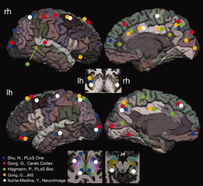
A summary of the top 20% most central nodes reported in the five prior studies. Since the tractography algorithms (i.e., probabilistic or streamline), templates (i.e., AAL or FreeSurfer), as well as graph‐theoretic measures were different in different studies, the comparisons were only approximate. It can be seen that large variability exists in the top 20% most central nodes in the literature, with the most consistent findings observed in the precuneus and middle occipital gyri. The details of the methodology differences were listed in the Supporting Information Table S1. The positions of the marking circles are in the approximate locations. [Color figure can be viewed in the online issue, which is available at wileyonlinelibrary.com.]

Table I.

The Pearson correlations coefficients (R) of the graph‐theoretical measures (E_loc, degree, strength, and BC) within and between the three reconstructing methods (M1, M2, and M3)

R		M1				M2				M3
		E loc	Degree	Strength	BC	E loc	Degree	Strength	BC	E loc	Degree	Strength	BC
M1	E loc		0.95	0.91	0.70	0.75	0.77	0.53	0.29	0.75	0.83	0.73	0.73
	Degree			0.90	0.70	0.73	0.80	0.51	0.32	0.72	0.86	0.71	0.73
	Strength				0.81	0.74	0.77	0.57	0.34	0.71	0.79	0.73	0.73
	BC					0.63	0.67	0.50	0.40	0.53	0.63	0.56	0.80
M2	E loc						0.94	0.85	0.45	0.89	0.89	0.89	0.71
	Degree							0.78	0.50	0.80	0.94	0.81	0.74
	Strength								0.57	0.76	0.73	0.85	0.60
	BC									0.32	0.45	0.39	0.55
M3	E loc										0.87	0.96	0.61
	Degree											0.86	0.73
	Strength												0.65
	BC

The correlations coefficients of the various graph‐theoretical measures within each individual tractography method were given in bold. All the correlation coefficients were statistically significant (P < 0.05). E _loc: local efficiency; BC: nodal betweenness centrality.

The discrepancies in the literature raise a fundamental issue that requires further investigation, namely, the degree to which the specific method used to compile the connectivity matrix influences small‐world properties and hub identification [Gong et al., 2009b; Iturria‐Medina et al., 2010]. For instance, structural connectivity maps can be generated from probabilistic tractography by initiating tracking from either gray matter or from deep white matter, and these two methods might produce different results. This is partially due to the fact that probabilistic tractography methods based on Monte Carlo sampling of voxelwise probability density functions (pdfs) suffer from distance‐related artifacts due to the progressive dispersion of uncertainty along the tracking path, giving a preferential weighting of regions close to the tracking start point at the expense of more distant areas. As a result, the probability map always demonstrates a decrease in probability values with distance from the start point of the seed region. Therefore, when the seed region is located in gray matter for tracking, the resulting connectivity matrix may be more weighted towards connections between the brain areas linked by short pathways. In contrast, when the seed region is located in the deep white matter [Jbabdi et al., 2010], connections between brain areas linked by long white‐matter pathways will have more seed voxels located on these pathways and therefore more samples sent from them, causing generally stronger connections between the regions linked by long tracts, another distance‐related effect that cannot be simply corrected by normalizing for the tract length (see Fig. 2).

Figure 2.

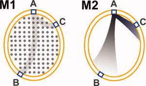
Schematic illustration of the connectivity bias introduced by different reconstruction methods. In M1 (left), when the whole‐brain white matter is used as the seed voxels (the gray dots), the connections between two remote brain regions (such as A and B), will have more seed voxels located on the possible pathways compared with those pathways among close brain regions (such as A and C), causing more samples sent for tracking and therefore stronger connectivity; By contrast, in M2 (right), when the GM/WM interface brain regions (blue squares) are used as the seed voxels for tracking, the progressive dispersion of uncertainty along the tracking path will give a preferential weighting of the connections between the close brain regions(such as A and C), in comparison with the remote brain regions (such as A and B). As a consequence, the NCD between three brain regions will have the order NCD_A–B > NCD_A–C in M1, but NCD_A–B < NCD_A–C in M2, a difference completely caused by the reconstruction method. [Color figure can be viewed in the online issue, which is available at wileyonlinelibrary.com.]

In this study, we quantitatively compared three methods for reconstructing connections from probabilistic tractography, using a same set of diffusion MRI data, to systemically assess their effects on the resulting connectivity matrix, and specifically, their effects on small‐world indices, identification of hubs, and hemispheric asymmetry in connectivity patterns. We hypothesized that the graph‐theoretic measures would be moderately correlated across the three methods, but despite this there would be large between‐method differences in small‐world indices and hub identification. We further hypothesized that if distance effects were one of the major reasons for between‐method discrepancies, results that are more consistent across methods should be obtained in analyses for hemispheric asymmetries in connectivity patterns, where the paired tracts in the two hemispheres are expected to have similar lengths.

METHODS

Subjects

Ninety‐four healthy right‐handed human subjects (age: 24.2 ± 0.84 yrs, 48 females) were recruited in this study after informed written consent as per Emory Institutional Review Board guidelines. All subjects had no history of neurological or psychiatric disorders.

Acquisition of MRI Data and Preprocessing

Human diffusion MRI

MRI was performed in a Siemens 3T Trio scanner (Siemens Medical System, Malvern, PA) with an twelve‐channel parallel imaging phase‐array coil. Foam cushions were used to minimize head motion. High‐resolution T1‐weighted images were acquired with a 3D magnetization‐prepared rapid gradient‐echo (MPRAGE) sequence for all participants. The scan protocol, optimized at 3T, used a repetition time/inversion time/echo time of 2600/900/3.02 msec, a flip angle of 8°, a volume of view of 240 × 256 × 176 mm³, a matrix of 240 × 256 × 176, and a resolution of 1 × 1×1 mm³, with 1 average. Total T1 scan time was ∼10 min.

Diffusion MRI data were collected with a diffusion‐weighted spin‐echo echo planar imaging (EPI) sequence with GRAPPA (factor of 2). A dual spin‐echo technique combined with bipolar gradients was used to minimize eddy‐current effects [Alexander et al., 1997]. The parameters used for diffusion data acquisition were as follows: diffusion‐weighting gradients applied in 60 directions with a b value of 1,000 sec/mm²; repetition time/echo time of 13,100/98 msec; field of view of 230 × 230 mm²; matrix size of 108 × 128; resolution of 2 × 2 × 2 mm³; and 64 slices with no gap, covering the whole brain. Averages of two sets of diffusion‐weighted images with phase‐encoding directions of opposite polarity (left–right) were acquired to correct for susceptibility distortion [Andersson et al., 2003]. For each average of diffusion‐weighted images, four images without diffusion weighting (b = 0 sec/mm²) were also acquired with matching imaging parameters. The total diffusion MRI scan time was ∼20 min.

Post‐mortem macaque diffusion MRI data

Diffusion MRI data were acquired in a formalin‐fixed post‐mortem macaque (Macaca mulatta) brain using a Bruker 9.4T scanner. A 2D spin echo MRI sequence was implemented at 0.55 mm isotropic resolution with an echo time of 22.25 μsec, a b value of 2,000 sec/mm², and 60 diffusion directions. We acquired three sets of diffusion‐weighted data for subsequent averaging. The total scan time was 72 hours.

Regions of macaque cortex were partitioned using the LVE00a scheme implemented in Caret 5.5 software (http://brainvis.wustl.edu/wiki/index.php/Main_Page) [Lewis and Van Essen, 2000], similar to the method used by Parkes et al., [2010]. To use this cortical partitioning scheme in our dataset, the FNIRT nonlinear normalization toolbox available in Oxford Center for Functional MRI of the Brain's Software Library (FSL, http://www.fmrib.ox.ac.uk/fsl/) was used to spatially match the single macaque F99UA1 MRI brain volume in the Caret 5.5 to our post‐mortem macaque brain. Then, the nonlinear warping transformation was applied to the LVE00a partitioning scheme to transfer the parcellated LVE00a cortical regions to the diffusion space of our post‐mortem macaque brain. Lastly, similar procedures for data preprocessing were applied to both human and macaque diffusion MRI data sets (see below for details).

Data preprocessing

Both human and macaque anatomical and diffusion MRI data were analyzed using FSL. T1‐weighted images of the human data were preprocessed with skull stripping [Smith, 2002], intensity bias correction [Zhang et al., 2001], noise reduction [Smith and Brady, 1997], and contrast enhancement (squaring the images and then dividing by the mean). Diffusion MRI data of the both species were first corrected for eddy‐current distortion. For human diffusion MRI data, susceptibility distortion was corrected following the method of Andersson et al. [2003] using Matlab (Matlab7, Mathworks) codes incorporated in SPM5 (http://www.fil.ion.ucl.ac.uk/spm/).

Reconstructing Anatomical Interregional Connectivity of Brain Networks

In this study, three tractography methods, denoted here as Method 1 (M1), method 2 (M2), and method 3 (M3), were employed to reconstruct the anatomical connectivity of brain networks for both datasets (human and macaque). The basic graph‐theoretic measures used to characterize brain networks, the procedures to derive the connectivity networks, and the differences among the three reconstruction methods will be described in details in the following section.

Node definition

The node is the most basic element of a network and its definition has a direct influence on the outcome of the network connectivity analysis [Sporns et al., 2005]. For the human subjects, FreeSurfer (http://surfer.nmr.mgh.harvard.edu/) was employed to parcellate each individual's high‐resolution T1‐weighted image into 82 regions (41 for each hemisphere), with each region representing a node of the connectivity matrix. As the fiber coherence in gray matter is low and it is not robust to start tracking using gray matter as the seed mask, a layer of voxels with the thickness of 2 mm between the gray matter and white matter, termed the gray/white‐matter (GM/WM) interface mask, of the 82 brain regions was generated to make tractography robust. An advanced post‐registration technique proposed by Andersson et al., [2003] was used in this study to correct susceptibility‐induced distortion in human diffusion MRI data, after which no discernable mismatch between each subject's T1‐weighed image and the corresponding diffusion MR image could be observed after a rigid‐body registration (six degree of freedom). This made it appropriate to include 14 subcortical regions (7 for each hemisphere) in our analyses, where (i) the size of these regions were small and (ii) they are located in more inferior part of the brain and therefore more prone to susceptibility‐induced distortion. After each subject's cortical and subcortical regions were derived, they were transformed into each subject's diffusion space for tractography using a rigid body transformation with six degree of freedom. Identical brain cortical and subcortical regions were used for the three reconstruction methods.

Deriving interregional connectivity map of brain networks

The procedure of deriving the interregional connectivity map of brain networks is illustrated in Figure 3. Probabilistic tractography implemented in FDT (http://www.fmrib.ox.ac.uk/fsl/), a diffusion toolbox in FSL, was modified to derive the interregional connectivity map, as the algorithm provides a mechanism to quantify the uncertainty due to noise, artifacts present in the MR scans, and the incomplete modeling of the diffusion signal. The derivation of the anatomical connectivity map of brain networks involved three steps [Behrens et al., 2003, 2007]:

• 1The local probability density functions (pdfs) of the principal diffusion direction in each voxel of the diffusion MRI data were generated through Markov Chain Monte Carlo sampling technique, using “bedpostX” in FSL and denoted as P(θ, φ|Y), where Y is the data and θ and φ define the principal diffusion direction in spherical coordinates.
• 2Tracking was started from one seed voxel and propagated based on the underlying pdfs estimated in step (1): for each random sample starting from the seed voxel, a principal diffusion direction (θ, φ) was sampled from P(θ, φ|Y) and then moved a distance s along (θ, φ). This process was repeated until the stopping criteria were met. For all three methods, the stopping criteria were set identical as those in the default settings in FSL, that is, when the streamline reached the termination masks, targets, propagating in a loop, etc. By repeating this step, a streamline fiber that took full account of the uncertainty in each propagation step could be derived and is termed a “probabilistic streamline” here to differentiate with the “streamline” used in the conventional deterministic tractography [Behrens et al., 2003]. At the voxels where multiple fiber orientations were detected [Behrens et al., 2007], the starting diffusion direction was randomly selected from one of the respective fiber pdfs.
• 3Seed masks were generated using each of the three different methods (M1, M2, and M3). In M1, whole‐brain white matter was segmented using FreeSurfer, which was then used as the seed mask. The source codes of the “probtrackx” in FSL were modified for counting the connectivity in this method. Two thousand random samples from each voxel of the white‐matter seed mask were sent and for each sample, a “probabilistic streamline” was propagated in both directions until they each reached a different brain target at which point, a connection between the two targets was counted for connectivity matrix. In M2, the GM/WM interface masks of the 82 brain regions were used as the seed masks: for each pair of brain regions, 2,000 samples per voxel were sent from the GM/WM interface seed mask, and the total number of “probabilistic streamlines” started from the GM/WM interface seed region and reached the GM/WM interface target region in that pair were summed and counted. The procedure was repeated again with the seed region and target region reversed. In M3, the tracking procedure was identical to M2. However, instead of counting the number of “probabilistic streamlines” connecting each seed and target‐region pair for the index of the connectivity strength, the derived tract volume was first (i) thresholded by a percentage of the total samples sent during the tracking process for that cortical region pair (0.02% was used in the present results, but a series of other thresholds were also tested), and then (ii) binarized to calculate the thresholded tract volume. This thresholded tract volume, encoding the information of connectivity strength, tract volume, surface areas of the cortical region pairs, and distance between them were subsequently employed as the index for the strength of connectivity of the each GM/WM interface region pairs in M3.

Figure 3.

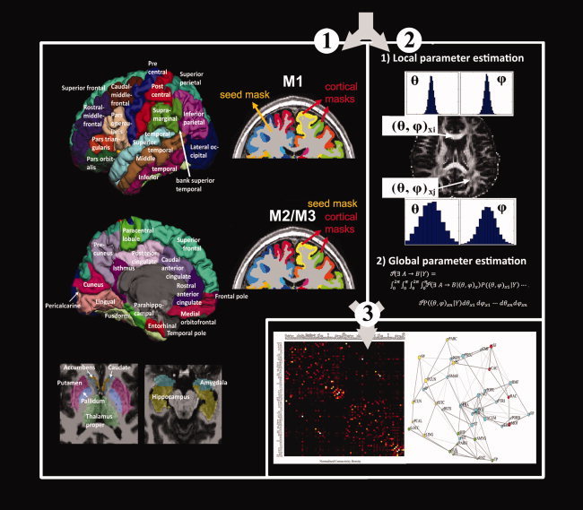
Procedure for reconstructing brain networks using diffusion probabilistic tractography. First, the T1‐weighted images were parcellated into 82 cortical and subcortical brain regions and seed masks located either in deep white matter (M1) or at the GM/WM interface (M2 and M3) were used for tractography (1); Second, probabilistic tractography implemented in FSL was used to derive the interregional connectivity map among different brain regions. The local orientation pdfs on each voxel were estimated, and then global connectivity was derived by sampling from the local pdfs. When a “probabilistic streamline” connected two different brain regions, it was counted and considered to contribute one unit to the total connectivity map (2). Lastly, interregional connectivity maps were derived based on the probabilistic tractography outputs. The topology of brain networks was reconstructed and analyzed using graph‐theoretic methods (3). [Color figure can be viewed in the online issue, which is available at wileyonlinelibrary.com.]

Constructing interregional connectivity map of the human brain

Maps of the interregional connectivity for human and macaque brains were created based on the outputs of the probabilistic tractography. Each GM/WM interface region became a node in the graph. Each connection between two brain regions became an edge. In M1 and M2, where the two end‐points of a “probabilistic streamline” were located in two different cortical regions (n _u, n _v), that specific probabilistic streamline sample was counted, contributing one unit to the connectivity strength of the edge [e _(u,v)]. After the total number of probabilistic streamlines was derived for each brain region pairs, it was divided by the mean of the areas of the two GM/WM interface regions , to normalize for the area differences across brain regions [Gong et al., 2009b; Hagmann et al., 2008]. In M3, the derived spatial distribution of the tract was thresholded by a certain percentage (0.02%) of the total number of samples sent from each brain region pair. The density measures using different methods were then normalized by the total values in the graph (i.e., the cost of the graph) to remove the global difference in each individual subject due to the various factors, such as the global organization differences due to aging, MR scan artifacts, “trackability,” etc. The intrinsic regional contrast of the network organization would be preserved after this global normalization. The resulting connectivity network was termed the graph of normalized connectivity density (NCD) for M1 and M2, and normalized tract volume density (NVD) for M3. Two brain regions with large NCD (NVD) were considered to have strong anatomical connections and those regions with NCD (NVD) close to 0 were not considered to have plausible anatomical connections.

Due to the probabilistic nature of the tractography algorithm used in this study, the majority of brain regions were shown to have non‐zero NCD (NVD), which is contrary to the classic anatomical view. The results must be thresholded, but the network density will change according to the threshold chosen. As there is currently no convention or theoretically motivated method, for specifying a threshold, we used series of thresholds ranging from network densities of 10–30%, with 50 intervals, to characterize the brain networks. These ranges give network densities similar to that of the previous studies [Achard and Bullmore, 2007; Gong et al., 2009b] and maximize the inclusion of real regional connections, while minimizing the number of false connections. As each of the network measures was computed at a specific threshold, we estimated the integrals of each metric curve, over the range of the different network densities, as a summary metric, as done in previous studies [Achard and Bullmore, 2007; Gong et al., 2009b].

Evaluation of the Performance of the Three Reconstruction Methods Using Post‐Mortem Macaque

The known macaque cortex structural connections derived by invasive tracer studies were extracted from the CoCoMac LVE00a database (http://www.cocomac.org) and used as a “gold standard” for evaluating the performances of the three reconstruction methods. Confirmed absence of a connection is denoted by a value of 0, while confirmed presence of a connection (irrespective of its strength or physiological characteristics) is denoted by a value of 1. Cortical regions with possible connections that were not investigated are denoted by a value of −1. The confirmed connections are modified so that they are bidirectional and symmetrical. After the interregional connectivity matrices of the macaque brain were derived using the three methods, a range of thresholds between 1 and 100% were applied on these NCD (NVD) networks and comparisons were made to the LVE00a atlas. A measure of accuracy, defined as the percentage of correctly determined connections (true positives) versus the percentage of incorrectly determined connections (false positives), was determined and plotted using a Receiver Operating Characteristic (ROC) curve implemented in Matlab (Matlab7, Mathworks).

Graph‐Theoretic Methods

Degree, strength and BC

The first local quantity used to characterize the brain connectivity network was the degree, defined as the number of connections to that node in the network, regardless of weight. Highly connected nodes have a large degree [Sporns et al., 2005]. A natural generalization of the degree to a weighted network is given by the strength, which is defined as the sum of the weights (NCD or NVD) of the connections from nodes that are connected to a given node i in a graph. Both degree and strength are local measures and therefore do not consider nonlocal effects, such as the existence of certain crucial nodes with small degree and/or strength but act as bridges between different subgraphs. In this context, a widely used quantity called nodal BC can be used to express the structural importance of these nodes. It is defined as the fraction of shortest paths between pairs of nodes that pass through a given node. Specifically, the BC of a weighted network is given as:

(1)

where σ${}_{\mathit{\text{kj}}}^{\mathit{\text{w}}}$ is the number of all shortest paths from node k to node j, and σ${}_{\mathit{\text{kj}}}^{\mathit{\text{w}}}$ (i) is the number of shortest paths passing through node i in a weighted graph.

In this study, the degree, strength, and BC within and across methods were compared to investigate their correlations. All the graph‐theoretic measures were calculated using the Matlab functions implemented in Brain Connectivity Toolbox (http://www.brain-connectivity-toolbox.net) [Rubinov and Sporns, 2010].

Small‐world properties

The small‐world network concept was first proposed by Watts and Strogatz, [1998] to describe many biological and technological networks that lie between completely random and regular networks. This concept was later expanded to both unweighted and weighted graphs, as well as to disconnected and nonsparse graphs [Latora and Marchiori, 2001, 2003]. Global and local efficiency instead of the characteristic path length and the cluster coefficient were used to characterize small‐world properties of networks in this study as these measures are valid for both weighted, nonweighted, disconnected, and nonsparse graphs [Latora and Marchiori, 2003]. Global efficiency of the graph G is defined as the average efficiency of the node i, which equals to the sum of the inverse of the harmonic mean of shortest path length (d _ij) between each pair of nodes within the network:

(2)

The local efficiency, however, is defined to characterize the local properties of the graph (G) by evaluating the efficiency of the subgraph of the neighbors of node i:

(3)

where E _loc,i is the local efficiency of node i, and d _jh(N _i) is the length of the shortest path between j and h, with only the neighbors of i included. It represents the extent to which the network is fault tolerant, measuring how efficient the information flow is within the first neighbors of a given node i when the node i is removed. Based on these two efficiency measures, the definition of a small‐world network could be assessed according to the information flow at global and local levels, which is characterized by high global (close to the global efficiency of the matched random networks) and local efficiency (much higher than the local efficiency of the matched random networks)[Latora and Marchiori, 2003]. The matched random networks were computed based on null‐hypothesis networks, with random topology but sharing the size and degree distribution of the original networks [Maslov and Sneppen, 2002; Rubinov and Sporns, 2010]. In this study, we compared the global and local efficiency of the interregional connectivity networks derived using the three reconstruction methods (M1, M2, and M3) with those derived from the matched random networks. Additionally, we conducted statistical analysis on the integrated, global (E _glo) and local efficiency (E _loc) as well as the scaled global (E _glo/E _{glo_random}) and local (E _loc/E _{loc_random}) efficiency of the derived brain networks to investigate the small‐world differences across the three reconstruction methods.

Identification and classification of community structure

Complex networks usually consist of several modules, in which the nodes densely interconnect with other nodes within the module, but relatively sparsely connect with the nodes outside the module. In this study, the different modules within the brain networks derived using the three methods were detected and classified based on the algorithm proposed by Newman [2006b] and the community structures of the three brain networks were plotted and compared.

The Relationship Between NCD (NVD) and Fiber Length

One possible explanation for differences in graph‐theoretic measures across the three methods could be differences in their sensitivity to distance. For example, one method might weight connections more between remote brain regions than the other methods. To evaluate this possibility, we first explored the relationships between NCD (NVD) and fiber length using simulated diffusion MRI data. Diffusion MRI data for white‐matter tracts with the same diameter, but varying lengths (4−160 mm) and fractional anisotropy (FA = 0.2, 0.7), were generated to simulate tracts with different lengths and degrees of fiber coherence. Then, the three reconstruction methods were applied to the simulated diffusion MRI data to determine whether the NCD (NVD) in the connectivity matrices correlated with fiber length and whether the correlations were similar across method. SNR similar to that in the in vivo diffusion MRI data (SNR = 15 for diffusion weighted images) and tensor profiles simulating single fiber pathway were used for all the simulations in this study.

After the interregional connectivity maps for all the human subjects were derived, we calculated the mean fiber length of the tracts contributing to the top 20% NCD (NVD) for each node in the brain networks and compared the results across the three methods. We hypothesized that if one method weights more toward the connectivity between two remote brain regions (i.e., connections linked by long fiber tracts) than that between two close ones, then the average of the mean fiber length of the white‐matter tracts that contribute to the top 20% NCD (NVD) in the connectivity matrix should be longer in that method. Therefore, based on the simulation results, we expected that the average mean fiber length of the tracts contributing to the top 20% NCV/NVD for all brain regions should have the order M1 > M3 > M2.

RESULTS

Evaluation of the Performance of the Three Reconstruction Methods Using Post‐Mortem Macaque Data

To evaluate the performance of the three methods, we compared the macaque interregional connectivity maps derived from diffusion tractography with the connectivity information extracted from invasive tracer studies. Figure 4A illustrates the partitioning scheme of LVE00a on a standard three‐dimensional (upper) and flat (lower) macaque brain. Figure 4B shows the connectivity information of the macaque data extracted from CoCoMac based on the invasive tracing studies. The results of the ROC curves that compare the connectivity matrices derived via the three methods with the cortico‐cortical information from invasive tracing studies for left and right hemispheres are presented in Figure 4C,D. No clear difference in performance among the three reconstruction methods was detected, which was further supported by the quantitative measure of the corresponding area under curve (AUC) in the ROC plots (M1‐left: 0.658; M1‐right: 0.645; M2‐ left:0.661; M2‐right:0.691; M3‐left: 0.705; M3‐right: 0.670). However, the order of the mean AUC from both hemispheres was shown to be M3 > M2 > M1, with M3 showing marginally higher accuracy on average compared to M1 and M2.

Figure 4.

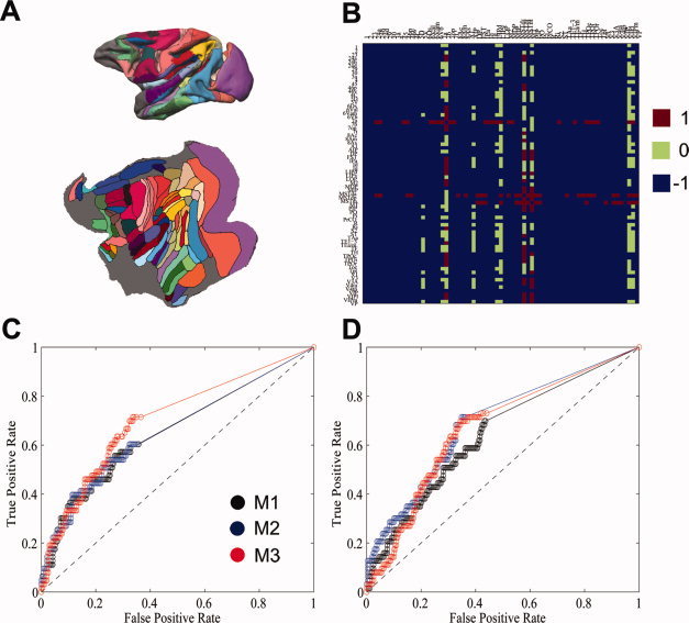
Comparison of anatomical connectivity matrices of post‐mortem macaque brain derived through invasive tracing studies and through diffusion probabilistic tractography technique. A: The partitioning scheme of LVE00a on a standard three‐dimensional (upper) and flat (lower) macaque brain. B: The anatomical connections derived by invasive tracer studies were extracted from CoCoMac LVE00a database (http://cocomac.org/home.asp). After the interregional connectivity matrices were derived using the three methods, a range of thresholds between 1 and 100% were applied on these NCD (NVD) networks and then compared with the LVE00a atlas. ROC curves for the left hemisphere (C) and right hemisphere (D) based on the three tractography methods were plotted and compared. No clear difference in performance was observed among three methods, although the mean AUC for M3 was marginally higher than that in M1 and M2, with order M3 > M2 > M1 (see Results section for details). Value 1 (0) has been used to indicate there is (not) a direct connection, while value −1 has been used to indicate that no connection information is available for the invasive tracer studies. The total 71 cortical regions compared in the present study include: 1, 2, 23, 24a, 24b, 24d, 29, 30, 3a, 4, 45, 46p, 46v, 4C, 5D, 5V, 6Ds, 6Val, 6Vam, 6Vb, 7a, 7b, 7op, 7t, 8Ac, 8Am, 8As, A1, AIP, DP, FST, IPa, Id, Ig, LIPd, LIPv, LOP, M2, MDP, MIP, MSTda, MSTdp, MSTm, MT, PIP, PO, Pi, PrCO, R, Ri, S2, ST, TAa, TE1‐3, TEa/m, TF, TH, TPOc, TPOi, TPOr, Toc, Tpt, V1, V3, V3A, V4ta, V4tp, VIP, VIPl, VIPm, VP. [Color figure can be viewed in the online issue, which is available at wileyonlinelibrary.com.]

Comparison of Small‐World Properties of the Interregional Connectivity Map of the Human Brain Across the Three Reconstruction Methods

Figure 5 shows the network density as a function of thresholding, and the local and global efficiency, as a function of network density for the three reconstruction methods. As expected, the network density decreased as the threshold became more stringent (Fig. 5A,D,G). Consistent with the previous studies [Gong et al., 2009b; Latora and Marchiori, 2003], all three networks showed high local (much higher than that of the matched random networks) and global efficiency (close to that of the matched random networks), indicating that the derived interregional connectivity maps in this study can be characterized as small‐world networks. Regarding the between‐method differences in small‐world indices, the integrated, original global, and local efficiency were first investigated: Kruskal‐Wallis tests rejected the null hypothesis that the integrated, original global efficiency (E _glo, P < 9.65e‐13) and overall local efficiency (E _loc, P < 1e‐20) in the three reconstruction methods were drawn from the same population. The post‐hoc sign rank test showed that the medians of the integrated, original global efficiency from M1, M2, and M3 has the order of M1 > M3 > M2 (M1 vs. M2: Z _(2,93) = 7.59, P < 2.57e‐11; M1 vs. M3: Z _(2,93) = 3.65, P < 4.35e‐04; M2 vs. M3: Z _{(2, 93)} = 2.47, P < 0.02). We also investigated the integrated, scaled global (E _glo/E _{glo_random}) and overall local efficiency (E _loc/E _{loc_random}) across the three methods: Similarly, Kruskal‐Wallis test rejected the null hypothesis that the integrated, scaled global efficiency (E _glo/E _{glo_random}, P < 1.11e‐16), and overall local efficiency (E _loc/E _{loc_random}, P < 7.7e‐14) were drawn from the same population. The post‐hoc sign rank test showed that the integrated, scaled global efficiency from M1 and M2 had larger medians than M3, but had similar median between each other (M1 vs. M2: Z _(2,93) = 0.68, P < 0.49; M1 vs. M3: Z _(2,93) = 8.37, P < 5.57e‐17; M2 vs. M3: Z _{(2, 93)} = 8.35, P < 6.77e‐17).

Figure 5.

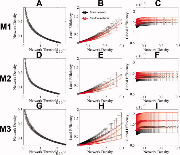
The small‐world properties of the interregional connectivity maps of the human brain. The network density, local efficiency and global efficiency are shown in A, B, C (for M1), D, E, F (for M2), and G, H, I (for M3). The network density ranges from 5 to 30%. The local and global efficiency of the derived interregional connectivity maps in this study match the description of networks with small‐world properties: high local (much higher than that of the matched random networks) and global (close to that of the matched random networks) efficiency. Both local efficiency and global efficiency of the interregional connectivity maps at the thresholds used for integration in our study (10–30%) in all three methods were significantly different from that in the matched random networks (two sample t‐tests with P < 0.05, two tails). Circles and the error bars represent the mean and one standard deviation of each measure across subjects. [Color figure can be viewed in the online issue, which is available at wileyonlinelibrary.com.]

Comparisons of Graph‐Theoretic Measures from the Three Reconstruction Methods

Degree, strength, and BC derived from the interregional connectivity maps are listed in Figure 6, 7, 8. Degree, strength, and BC were sorted based on their order in M1, then applied to M2 and M3 for visual comparisons. The four graph‐theoretic measures, that is, the local efficiency, degree, strength, and BC, were shown to be correlated with each other within each method (mean R _{all_within} = 0.76, see Table I for details), with BC having the lowest correlation coefficients among the four local graph measures (mean R _{BC_within} = 0.63), which is in good accordance with a previous study [Sporns et al., 2007]. We also observed that the graph‐theoretic measures across the three methods were interrelated (mean R _{all_between} = 0.67), with BC again having the lowest correlation coefficients (mean R _{BC_between} = 0.58).

Figure 6.

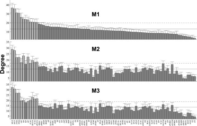
Comparisons of the degree of the interregional connectivity maps derived using the three different reconstruction methods. The order of the degree for different brain regions were based on M1 and then were applied on M2 and M3. The solid vertical bars and error bars represent the mean and standard deviation of the degrees across the subjects. The horizontal solid and dashed lines denote the mean and mean plus one standard deviation across all brain regions. Brain regions with measures larger than the mean plus one standard deviation are highlighted with light gray color.

Figure 7.

Comparisons of the strengths of the interregional connectivity maps derived using the three different tractography methods. The order of the strengths for different brain regions were based on M1 and then were applied on M2 and M3. The solid vertical bars and error bars represent the mean and standard deviation of the degrees across the subjects. The horizontal solid and dashed lines denote the mean and mean plus one standard deviation among various brain regions. Brain regions with measures larger than the mean plus one standard deviation is highlighted with light gray color.

Figure 8.

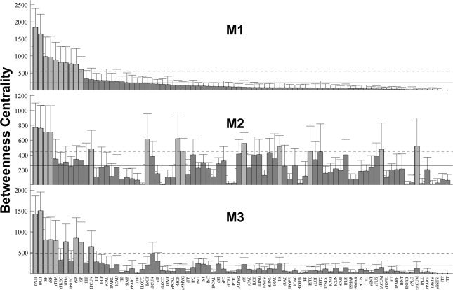
Comparisons of the BC of the interregional connectivity maps derived using the three different tractography methods. The order of the BCs for different brain regions were based on M1 and then were applied on M2 and M3. The solid vertical bars and error bars represent the mean and standard deviation of the degrees across the subjects. The horizontal solid and dashed lines denote the mean and mean plus one standard deviation among various brain regions. Brain regions with measures larger than the mean plus one standard deviation is highlighted with light gray color.

The nodes with the top 20% highest BC values derived in the M1, M2, and M3 were considered as hubs in this study and marked in Figure 9. Among the 16 nodes (top 20% of 82 nodes) with highest BC, bilateral putamen, bilateral superior frontal cortex, and left precuneus were identified as hubs in all three reconstruction methods, consisting of ∼31% of the selected nodes.

Figure 9.

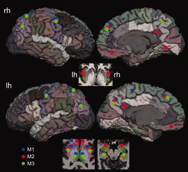
A summary of the top 20% nodes with the highest nodal BC values derived in the present study. The same diffusion MRI data, partitioning scheme were used in all three reconstruction methods. Large variability can be observed from the most central nodes (20%) based on the ranks of BC measures. The bilateral putamen, bilateral superior frontal lobes, and left precuneus were unanimously identified as hubs in all three methods. The positions of the marking circles are in the approximate locations. [Color figure can be viewed in the online issue, which is available at wileyonlinelibrary.com.]

The community structure of the brain networks derived using the three methods are shown in Figure 10. It can be observed that the module numbers as well as the nodes included within each module varies across the three methods. The topological connectivity backbone in M1 seems to show stronger connections among the remote brain regions compared to that in M2 and M3. For example, the nodes located at the medial posterior parietal regions in M1 tend to have less degree and weaker NCD among themselves than M2 and M3.

Figure 10.

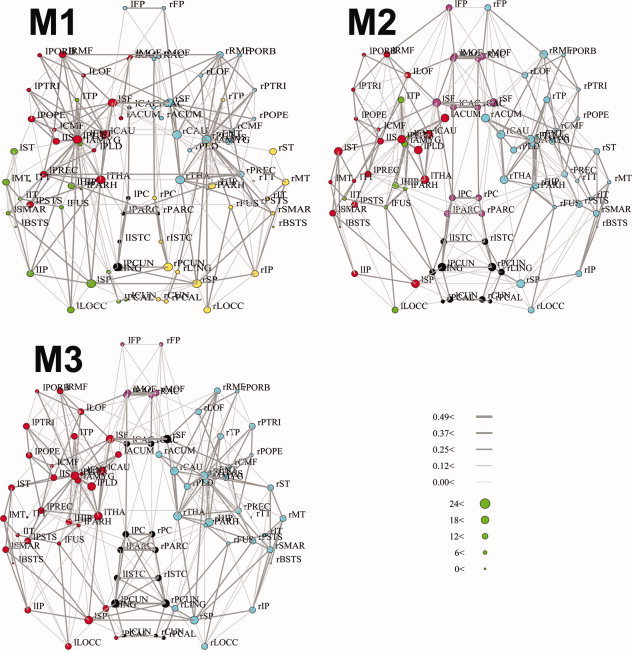
Dorsal view of the connectivity backbone derived using the M1, M2, and M3 in anatomical coordinates. Nodes are coded according to the degree and edges are coded according to the strength of NCD (NVD). The community structure of the network was obtained through subdividing the network into nonoverlapping modules, based on the algorithm proposed by Newman [2006a]. Different modules in networks were coded using different color schemes, which do not have a one‐to‐one correspondence across the three methods, as the number and size of the clusters detected were different across methods. The full name of the abbreviations used in the figures could be found in the Supporting Information Table II (Table S2). r: right hemisphere; l: left hemisphere.

The Relationship Between the NCD (NVD) and Fiber Length in the Simulated and In Vivo Diffusion MRI Data

We generated two sets of diffusion MRI data simulating white‐matter tracts with different fiber coherence and length (Fig. 11). The preliminary results demonstrated that when the fiber coherence was high (FA = 0.7), the NCD in both M1 and M2 showed a clear distance‐related effect (Fig. 11A, M1: y = 0.001x + 1.24e‐5, R ² = 0.99; M2: y = 0.42x ^−0.43 + 0.04, R ² = 0.95), indicating a possible bias in NCD for M1, favoring the connections between remote brain regions by longer white‐matter tracts, and vice versa for M2. In contrast, no significant distance effect was seen between the NVD and fiber length in M3 (Fig. 11A, y = −1.5⁻⁵ x + 0.12, R ² = 0.02). When fiber coherence was low (FA = 0.2), the NCD and NVD in all three methods decreased significantly as fiber length increased and dropped off to zero when the fibers were longer than 65 mm (Fig. 11B).

Figure 11.

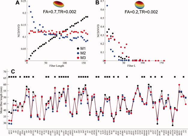
The relationships between the NCD (NVD) and fiber length in the simulated and in vivo diffusion MRI data; (A) a clear distance effect on the NCD (NVD) could be seen in M1 and M2, when fibers were coherent. This distance effect was not as significant in M3 (see Result section for details); (B) when the coherence of the white matter tracts was low, a similar distance effect was seen in all three methods, that is, probability decreased significantly with distance, and dropped off to zero for the fibers longer than 65 mm; (C) The mean fiber lengths of the white‐matter tracts that contributed to the top 20% NCD (NVD) for each brain region were plotted across the three methods. Consistent with the observations in our simulations, there were significant differences in the mean fiber length of the tracts that contributed to the top 20% NCD (NVD) for each brain region. Among 82 brain regions, 45% of them have the mean fiber length in M3 shorter than that in M1 but longer than in M2, a representation much higher than the proportion by a random chance (17%). Black squares in Fig. 11C denote the brain regions with the order of mean fiber length M1 > M3 > M2. [Color figure can be viewed in the online issue, which is available at wileyonlinelibrary.com.]

The mean fiber length of the white matter tracts that contribute to the top 20% NCD (NVD) for each brain region in the in vivo MRI data was plotted and compared across the three reconstruction methods (Fig. 11C). Consistent with our simulations, there were significant differences in mean fiber length: 37 (45%) out of the 82 brain regions in M3 have the mean fiber length ranging between M1 and M2 with the order of M1 > M3 > M2, a representation much higher than the proportion by a random chance (14 regions, 17%).

Hemispheric Asymmetry in Connectivity Patterns

The interregional connectivity maps of brain networks characterized by graph‐theoretic measures, such as E _glo and BC, were used to evaluate hemispheric asymmetry in connectivity patterns in humans. The detailed statistics are listed in Table II. In brief, no hemispheric asymmetry in connectivity patterns in terms of E _glo was detected with either M1 or M2, whereas left > right global asymmetry was found with M3. As regards regional differences in connectivity patterns, the majority of the asymmetrical brain regions identified in M2 showed left > right asymmetry, whereas roughly the same amount of left > right and right > left brain regions were identified using M1 and M3. The precuneus was the only brain area identified by all three methods with left > right asymmetry (see Table II for details).

Table II.

The statistic results of the regional brain asymmetry in connectivity patterns indexed by the graph‐theoretic measures E _glob and BC

	Index		P values	Asymmetry
M1	E glob		0.7458	N/A
	BC	IP	3.92E‐06	R > L
		ACUM	3.01E‐06	R > L
		PORB	4.51E‐06	R > L
		SP	9.28E‐05	R > L
		FP	5.32E‐04	R > L
		POPE	0.006	R > L
		MOF	0.009	R > L
		TT	0.015	R > L
		PCUN	3.04E‐04	L > R
		PUT	6.20E‐04	L > R
		AMYG	0.002	L > R
		RMF	0.018	L > R
M2	E glob		0.070	N/A
	BC	IP	2.91e‐6	R > L
		LOCC	5.20E‐05	L > R
		RAC	8.45E‐05	L > R
		PCUN	2.98E‐04	L > R
		PC	0.0037	L > R
M3	E glob		0.009	L > R
	BC	RAC	6.98E‐08	R > L
		FP	2.64E‐04	R > L
		CUN	0.001	R > L
		SP	0.0013	R > L
		PCAL	0.0022	R > L
		MOF	0.0058	R > L
		TP	0.011	R > L
		FUS	1.14E‐05	L > R
		PCUN	6.29E‐05	L > R
		PC	3.15E‐04	L > R
		AMYG	0.0013	L > R
		PSTS	0.009	L > R
		CAC	0.011	L > R

DISCUSSION

In this study, we investigated the influence of connection reconstruction method on the interregional connectivity map of the human brain. Specifically, three reconstruction methods using diffusion probabilistic tractography were applied to the same diffusion MRI data set and interregional connectivity maps were derived and compared with respect to their small‐world properties, identification of hub regions, and hemispheric asymmetry in connectivity patterns. Brain anatomical networks showed robust small‐world properties regardless of the reconstruction method. However, significant differences in small‐world measures were detected across the three methods. In addition, large between‐method differences in the graph‐theoretic measures were observed, resulting in differences in hub identification as well as brain asymmetry patterns. This suggests that the choice of connection reconstruction method for probabilistic tractography must be considered as a confounding factor when comparing studies of interregional connectivity based on probabilistic tractography.

Evaluation of the Performance of the Three Methods Through Comparison With Macaque Post‐Mortem Data

Validating the structural connectivity patterns in the human brain using diffusion MRI data has always been challenging, as no gold standard for interregional connections in the human brain is currently available. Fortunately, the structural connectivity of macaque brains has been a subject of intense study using invasive tracing techniques [Felleman and Van Essen, 1991; Ferry et al., 2000; Lewis and Van Essen, 2000]. In the study by Lewis et al., the partitioning scheme investigated in the tracer study was also available digitally, allowing us to evaluate the validity of macaque cortico‐cortical connectivity maps obtained via diffusion tractography. Our preliminary results indicated that deriving the interregional connectivity map of the brain via tracking from deep white matter (as implemented in M1), where the uncertainty of the voxelwise pdfs is low, does not give significant benefits in accuracy compared to conventional tracking methods such as M2 [Gong et al., 2009b]. Similarly, none of the three methods was clearly superior to the others based on these results in postmortem macaque, although the M3 showed slightly higher accuracy on average compared to M1 and M2. However, we believe that this results are still preliminary and that further investigations are needed for several reasons: first, the gold standard we used here, that is, the invasive tracer study, explored majorly the parietal and temporoparietal cortico‐cortical connections, enabling us to validate only a small portion of the white‐matter connections in the brain (Fig. 4B); second, the connection information in the tracing study was binary (connections were scored present or absent), which did not accurately capture the strength of connections; lastly, considering the large between‐subject and between‐hemisphere variability in the connectivity matrix derived from diffusion tractography, future studies with larger sample sizes are desired to draw a statistical conclusion on the performance of the three methods.

The Effect of Fiber Length on Connectivity Maps

For any probabilistic tractography method that depends on Monte Carlo sampling to estimate the voxelwise pdfs [Behrens et al., 2003; Lazar and Alexander, 2005; Parker and Alexander, 2005], the probability of connections from a start voxel to a target one is defined as the frequency with which “probabilistic streamlines” pass through the target voxel, normalized for the total number of the “probabilistic streamlines” sent during the Monte Carlo random walk. Therefore, the connectivity map always demonstrates a decrease in probability values with distance from the start point of the seed mask. This is a result of the progressive dispersion of uncertainty due to noise, artifacts, and/or a genuine reflection of fiber spreading from voxel to voxel. Although this definition of probability is a valid representation of the likelihood of given “probabilistic streamlines” connecting two voxels, it can cause difficulty in interpreting the contrast in the connectivity strength between different brain areas connected by fiber tracts with various lengths. For example, when M2 is chosen to map structural connectivity information of the brain, the NCD would be lower for brain areas linked by long tracts (remote brain regions) than those by short ones, even though the actual connectivity strength of the two cases and all other conditions are kept the identical. This was clearly demonstrated in the simulation results (Fig. 11, M2): the NCD between two target regions decreased as fiber length increased, regardless the coherence of fibers (FA = 0.2, 0.7). Furthermore, the relationship between the NCD and fiber length is also determined by a variety of other parameters in diffusion MRI data, such as noise and artifacts in the MRI data, tract anatomy (fanning out or not), termination criteria for tracking, etc., making correction for the fiber length alone insufficient [Gong et al., 2009b; Iturria‐Medina et al., 2008].

Another alternative strategy is to initiate the tracking from each voxel in deep white matter, as implemented in M1 in this study [Hagmann et al., 2008; Jbabdi et al., 2010]. This approach was originally thought to be more robust, since the uncertainty of pdfs in deep white matter is usually considered low compared to that near gray matter. However, as the remote brain regions linked by long white‐matter tracts will have more seed voxels located on the tracts; more samples will be sent on the pathways for tracking, causing stronger connectivity between the two areas–another distance‐related effect in addition to the one in M2. Whereas this effect could be easily corrected in the conventional deterministic tractography, as it affects connectivity values linearly [Hagmann et al., 2008], the problem becomes more complicated in probabilistic tractography: as the voxelwise pdfs in probabilistic tractography have a distribution instead of a binarized values (with the probability of either 1 or 0) as in deterministic tractography, the relationship between NCD and fiber length can no longer be simply modeled as linear. Instead, the NCD is affected by both the biases due to the different number of seeds sent for tracking and the progressive dispersion of “probabilistic streamline” samples as they propagate. To test this point, we employed the simulated white‐matter tracts as a simplified model: when the NCD reconstructed using M1 was corrected by tract length, the relationship between tract‐length‐normalized NCD and tract length still presented, and became highly similar as that in M2 (see Supporting Information Fig. 4). This clearly demonstrated that simply normalizing the NCD in M1 as that in deterministic algorithms would not alleviate the distance‐related effect associated with the method.

One approach that could potentially mitigate the distance effect is to start tracking from the GM/WM interface, as in M2, but to use the thresholded tract volume as the index of connectivity; we implemented this approach in M3. We reasoned that even though two distant brain regions with long tracts connecting them have reduced connectivity due to the dispersion of the local pdfs, the increased tract volume could partially compensate for the decreased probability, making the NVD insensitive to the distance between brain regions. By using a percentage of the total samples sent for tracking to threshold the tract volume, the resultant thresholded tract volume should be a value encoding the information containing both tract strength and volume, possibly serving as a more representative index for brain mapping studies. The relative insensitivity of M3 to distance could be appreciated in both the simulations (Fig. 11A,B) and the in vivo data (Fig. 11C): Compared to the NCD in M1 and M2, we observed smaller distance‐related effects on the NVD in M3. In the in vivo diffusion MRI data, the mean length of the tracts in M3 that contribute to the top 20% NVD for each node was lower than for the NCD in M1, which tends to weigh more toward connections between distant brain regions, but higher than that in M2, which has been shown to favor connections between close brain regions.

It is obviously not trivial to correct the distance effect inherent in any brain mapping study that relies on probabilistic tractography for compiling the interregional connectivity maps and it has been suggested that the flux of connections in the probability should obey a probabilistic version of Gauss's Law, which means that the probability at a distance could be expressed in terms of the surface area of the isofrequency contour. However, this analogy with Gauss's Law is only approximate in practice due to computational effects such as use of stopping criteria during tracking, geometric effects (brain‐CSF interface), and tract anatomy [Morris et al., 2008]. For example, in one of our tests to derive the null probability map in a homogenous diffusion phantom in which we sent 50,000 samples on a seed voxel, no “probabilistic streamline” tract could propagate beyond 50 mm from the start voxel with the stopping criteria same as the default settings in FDT toolbox, an obvious violation of the approximation (results not shown).

Hub Identification and Brain Asymmetry in Connectivity Patterns

Compiling interregional connectivity maps of brain networks involves complex procedures that require careful selection of a series of parameters–ranging from the tracking algorithm, to cohort size, to partitioning schemes, to inclusion or exclusion of subcortical regions, to number of diffusion directions–all of which have been shown to potentially influence the properties of the resulting connectivity maps [Gong et al., 2009b; Hagmann et al., 2008; Vaessen et al., 2010; Wang et al., 2009; Zalesky et al., 2010]. As a result, we set all other factors constant in this study except for the reconstruction method and compared the interregional connectivity maps generated by the three different approaches. We observed that even though there were moderate to high correlations in graph‐theoretic measures across the three methods, they exhibited large differences in the identified hub regions. For the top 20% of the 82 brain regions with the highest BC values, only bilateral putamen, bilateral superior frontal cortex, and left precuneus were identified unanimously as hubs by all three methods, consisting of approximately one third of the selected 20% nodes. Of these three nodes, the precuneus is of particularly interest. The precuneus is involved in self‐referential processing, visuospatial imagery, episodic memory retrieval, and consciousness [Bullmore and Sporns, 2009; Cavanna and Trimble, 2006]. Similar to our results, it is also the only brain area unanimously identified as a hub region in all of the five previously published studies on hubs in humans, confirming its prominent structural role in brain networks. Interestingly, a closer look at the ranks of the precuneus based on BC values revealed that the mean rank of the precuneus in M3 (mean: 9.5, left: 9, right: 10) was higher than that in M1 (mean: 18, left: 12, right: 24) and M2 (mean: 16, left: 10, right: 22), respectively, perhaps another indication that using thresholded tract volume is a more representative measure than NCD in M1 and M2.

The selection of reconstruction method might also depend on the aims of the study itself. For instance, a method might not be capable of accurately capturing the contrasts of white‐matter connections among different brain areas, that is, identification of hub regions, due to its limitations in the distance‐related bias, but might still be sensitive enough to detect the differences between a brain region in the left hemisphere and its corresponding right one, that is, brain asymmetry in connectivity patterns, as both of them having similar geometric distances with other brain regions. To test this possibility, we conducted brain asymmetry analyses based on the interregional connectivity maps and compared the results. It is interesting to note that there were still large variations in the global and local measures across methods, indicating some factors other than distance contributing to the between‐method differences, which warrant future studies.

It is also worth noting that hubs in this model are identified solely by their anatomical connections in brain networks. Two identified hubs with similar importance based on the structural connectivity may have quite different functional fingerprints and/or biophysics (i.e., excitatory or inhibitory, conduction delay) [Sporns et al., 2005]. Therefore, characterizing and validating connectivity information of brain networks based on multimodality approach may depict a more comprehensive picture of hubs in brain networks [Honey et al., 2009]. Similarly, due to (i) the macroscale nature of the parcellation scheme used in this study and (ii) nonexistence of universally accepted parcellation template, we might have underestimated the importance of the brain regions that consist of multiple heterogeneous yet interconnected sub‐regions/‐nuclei, as the connectivity information of these local circuits could not be captured in this study. Therefore, we expect that the results in small‐world properties, hub identification, etc. will vary if the current three methods were applied by using a finer parcellation scheme, as indicated in the study by Zalesky et al. [2010]. The details regarding how node number affects the reconstructed brain network in terms of the distribution of hubs on the cerebral cortex is currently under investigation and will be reported in an independent publication.

The Importance of Including Subcortical Regions

With the advanced post‐processing method for correcting susceptibility distortion used in our study [Andersson et al., 2003], no visible spatial mismatch between a T1‐weighted anatomical image and its corresponding diffusion image was present after a rigid‐body registration (six degrees of freedom), making it possible to include even fourteen compact subcortical regions (17.1% of all the regions) in our analyses. Even though there is still controversy regarding how the subcortical areas should be included and weighted together with cortical regions for an unbiased brain network study [Hagmann et al., 2008], our results underlined the prominent structural role of the subcortical regions: among the top 20% nodes with the highest BC values, the subcortical regions constitute of 43.8% in M1, and 37.5% in M2 and M3, respectively, much higher than their representation as a proportion of the total number of brain regions included (17.1%). Therefore, structural and functional brain mapping studies that exclude subcortical areas may be missing important connections involving subcortical‐cortical coupling and/or cortico‐cortical circuits that loop through subcortical structures.

CONCLUSIONS

We applied three connection reconstruction methods based on probabilistic tractography for compiling interregional connectivity maps of brain networks on the same set of diffusion MRI data, and then compared the resultant connectivity matrices. Although there were moderate to high correlations among different graph‐theoretic measures in the three methods, significant between‐method variability in terms of small‐world properties, brain‐hub identification, and hemispheric asymmetry were demonstrated, suggesting that reconstruction method has a significant impact on derived brain networks. We also proposed that compared to the conventional connectivity index, using thresholded tract volume as the index for the strength of connectivity could alleviate the distance‐related effect that is common in brain mapping studies based on probabilistic tractography. Despite some between‐method inconsistencies in hub identification, the left precuneus was unanimously identified as a hub, in good agreement with prior studies, suggesting its prominent role in brain networks.

Supporting information

Additional Supporting Information may be found in the online version of this article.

Supporting Information

Supporting Figure 1

Supporting Figure 2

Supporting Figure 3

Supporting Figure 4

REFERENCES

- Achard S, Bullmore E ( 2007): Efficiency and cost of economical brain functional networks. PLoS Comput Biol 3: e17. [DOI] [PMC free article] [PubMed] [Google Scholar]
- Alexander AL, Tsuruda JS, Parker DL ( 1997): Elimination of eddy current artifacts in diffusion‐weighted echo‐planar images: the use of bipolar gradients. Magn Reson Med 38: 1016–1021. [DOI] [PubMed] [Google Scholar]
- Andersson JL, Skare S, Ashburner J ( 2003): How to correct susceptibility distortions in spin‐echo echo‐planar images: Application to diffusion tensor imaging. Neuroimage 20: 870–888. [DOI] [PubMed] [Google Scholar]
- Behrens TE, Woolrich MW, Jenkinson M, Johansen‐Berg H, Nunes RG, Clare S, Matthews PM, Brady JM, Smith SM ( 2003): Characterization and propagation of uncertainty in diffusion‐weighted MR imaging. Magn Reson Med 50: 1077–1088. [DOI] [PubMed] [Google Scholar]
- Behrens TE, Berg HJ, Jbabdi S, Rushworth MF, Woolrich MW ( 2007): Probabilistic diffusion tractography with multiple fibre orientations: What can we gain? Neuroimage 34: 144–155. [DOI] [PMC free article] [PubMed] [Google Scholar]
- Bullmore E, Sporns O ( 2009): Complex brain networks: graph theoretical analysis of structural and functional systems. Nat Rev Neurosci 10: 186–198. [DOI] [PubMed] [Google Scholar]
- Cavanna AE, Trimble MR ( 2006): The precuneus: A review of its functional anatomy and behavioural correlates. Brain 129( Pt 3): 564–583. [DOI] [PubMed] [Google Scholar]
- Felleman DJ, Van Essen DC ( 1991): Distributed hierarchical processing in the primate cerebral cortex. Cereb Cortex 1: 1–47. [DOI] [PubMed] [Google Scholar]
- Ferry AT, Ongur D, An X, Price JL ( 2000): Prefrontal cortical projections to the striatum in macaque monkeys: Evidence for an organization related to prefrontal networks. J Comp Neurol 425: 447–470. [DOI] [PubMed] [Google Scholar]
- Gong G, He Y, Concha L, Lebel C, Gross DW, Evans AC, Beaulieu C ( 2009a): Mapping anatomical connectivity patterns of human cerebral cortex using in vivo diffusion tensor imaging tractography. Cereb Cortex 19: 524–536. [DOI] [PMC free article] [PubMed] [Google Scholar]
- Gong G, Rosa‐Neto P, Carbonell F, Chen ZJ, He Y, Evans AC ( 2009b): Age‐ and gender‐related differences in the cortical anatomical network. J Neurosci 29: 15684–15693. [DOI] [PMC free article] [PubMed] [Google Scholar]
- Hagmann P, Cammoun L, Gigandet X, Meuli R, Honey CJ, Wedeen VJ, Sporns O ( 2008): Mapping the structural core of human cerebral cortex. PLoS Biol 6: e159. [DOI] [PMC free article] [PubMed] [Google Scholar]
- Honey CJ, Sporns O, Cammoun L, Gigandet X, Thiran JP, Meuli R, Hagmann P ( 2009): Predicting human resting‐state functional connectivity from structural connectivity. Proc Natl Acad Sci U S A 106: 2035–2040. [DOI] [PMC free article] [PubMed] [Google Scholar]
- Iturria‐Medina Y, Sotero RC, Canales‐Rodriguez EJ, Aleman‐Gomez Y, Melie‐Garcia L ( 2008): Studying the human brain anatomical network via diffusion‐weighted MRI and Graph Theory. Neuroimage 40: 1064–1076. [DOI] [PubMed] [Google Scholar]
- Iturria‐Medina Y, Perez Fernandez A, Morris DM, Canales‐Rodriguez EJ, Haroon HA, Garcia Penton L, Augath M, Galan Garcia L, Logothetis N, Parker GJ, Melie‐Garcia L. 2011. Brain hemispheric structural efficiency and interconnectivity rightward asymmetry in human and nonhuman primates. Cereb Cortex. 21:56‐67. [DOI] [PubMed] [Google Scholar]
- Jbabdi S, Behrens TE, Smith MS ( 2010): ICA‐based cortical parcellations using resting‐state fMRI and diffusion tractography. Annual Meeting of Human Brain Mapping, Barcelona, Spain, Jun 6–Jun 10.
- Latora V, Marchiori M ( 2001): Efficient behavior of small‐world networks. Phys Rev Lett 87: 198701 [DOI] [PubMed] [Google Scholar]
- Latora V, Marchiori M ( 2003): Economic small‐world behavior in weighted networks. Eur Phys J B 32: 249–263. [Google Scholar]
- Lazar M, Alexander AL ( 2005): Bootstrap white matter tractography (BOOT‐TRAC). Neuroimage 24: 524–532. [DOI] [PubMed] [Google Scholar]
- Lewis JW, Van Essen DC ( 2000): Corticocortical connections of visual, sensorimotor, and multimodal processing areas in the parietal lobe of the macaque monkey. J Comp Neurol 428: 112–137. [DOI] [PubMed] [Google Scholar]
- Li Y, Liu Y, Li J, Qin W, Li K, Yu C, Jiang T ( 2009): Brain anatomical network and intelligence. PLoS Comput Biol 5: e1000395. [DOI] [PMC free article] [PubMed] [Google Scholar]
- Maslov S, Sneppen K ( 2002): Specificity and stability in topology of protein networks. Science 296: 910–913. [DOI] [PubMed] [Google Scholar]
- Morris DM, Embleton KV, Parker GJ ( 2008): Probabilistic fibre tracking: differentiation of connections from chance events. Neuroimage 42: 1329–1339. [DOI] [PubMed] [Google Scholar]
- Newman ME ( 2006a): Finding community structure in networks using the eigenvectors of matrices. Phys Rev E Stat Nonlin Soft Matter Phys 74( 3 Pt 2): 036104. [DOI] [PubMed] [Google Scholar]
- Newman ME ( 2006b): Modularity and community structure in networks. Proc Natl Acad Sci U S A 103: 8577–8582. [DOI] [PMC free article] [PubMed] [Google Scholar]
- Parker GJ, Alexander DC ( 2005): Probabilistic anatomical connectivity derived from the microscopic persistent angular structure of cerebral tissue. Philos Trans R Soc Lond B Biol Sci 360: 893–902. [DOI] [PMC free article] [PubMed] [Google Scholar]
- Parkes LM, Haroon HA, Augarth M, Logothetis NK, Parker GJ ( 2010): High resolution tractography in macaque visual system‐validation against in vivo tracing. Proceedings of the Joint Annual Meeting of the International Society of Magnetic Resonance in Medicine. Stockholm, Sweden.
- Passingham RE, Stephan KE, Kotter R ( 2002): The anatomical basis of functional localization in the cortex. Nat Rev Neurosci 3: 606–616. [DOI] [PubMed] [Google Scholar]
- Rubinov M, Sporns O ( 2010): Complex network measures of brain connectivity: Uses and interpretations. Neuroimage 52: 1059–1069. [DOI] [PubMed] [Google Scholar]
- Shu N, Liu Y, Li J, Li Y, Yu C, Jiang T ( 2009): Altered anatomical network in early blindness revealed by diffusion tensor tractography. PLoS One 4: e7228. [DOI] [PMC free article] [PubMed] [Google Scholar]
- Smith SM ( 2002): Fast robust automated brain extraction. Hum Brain Mapp 17: 143–155. [DOI] [PMC free article] [PubMed] [Google Scholar]
- Smith MS, Brady JM ( 1997): SUSAN‐A new approach to low level image processing. Int J Comput Vision 23: 45–78. [Google Scholar]
- Sporns O, Tononi G, Kotter R ( 2005): The human connectome: A structural description of the human brain. PLoS Comput Biol 1: e42. [DOI] [PMC free article] [PubMed] [Google Scholar]
- Sporns O, Honey CJ, Kotter R ( 2007): Identification and classification of hubs in brain networks. PLoS One 2: e1049. [DOI] [PMC free article] [PubMed] [Google Scholar]
- Vaessen MJ, Hofman PA, Tijssen HN, Aldenkamp AP, Jansen JF, Backes WH ( 2010): The effect and reproducibility of different clinical DTI gradient sets on small world brain connectivity measures. Neuroimage 51: 1106–1116. [DOI] [PubMed] [Google Scholar]
- Wang J, Wang L, Zang Y, Yang H, Tang H, Gong Q, Chen Z, Zhu C, He Y ( 2009): Parcellation‐dependent small‐world brain functional networks: a resting‐state fMRI study. Hum Brain Mapp 30: 1511–1523. [DOI] [PMC free article] [PubMed] [Google Scholar]
- Watts DJ, Strogatz SH ( 1998): Collective dynamics of ‘small‐world’ networks. Nature 393: 440–442. [DOI] [PubMed] [Google Scholar]
- Zalesky A, Fornito A, Harding IH, Cocchi L, Yucel M, Pantelis C, Bullmore ET ( 2010): Whole‐brain anatomical networks: Does the choice of nodes matter? Neuroimage 50: 970–983. [DOI] [PubMed] [Google Scholar]
- Zhang Y, Brady M, Smith S ( 2001): Segmentation of brain MR images through a hidden Markov random field model and the expectation‐maximization algorithm. IEEE Trans Med Imaging 20: 45–57. [DOI] [PubMed] [Google Scholar]
Associated Data
This section collects any data citations, data availability statements, or supplementary materials included in this article.
Supplementary Materials