Multi-channel multi-scale fully convolutional network for 3D perivascular spaces segmentation in 7T MR images

Abstract

Accurate segmentation of perivascular spaces (PVSs) is an important step for quantitative study of PVS morphology. However, since PVSs are the thin tubular structures with relatively low contrast and also the number of PVSs is often large, it is challenging and time-consuming for manual delineation of PVSs. Although several automatic/semi-automatic methods, especially the traditional learning-based approaches, have been proposed for segmentation of 3D PVSs, their performance often depends on the hand-crafted image features, as well as sophisticated preprocessing operations prior to segmentation (e.g., specially defined regions-of-interest (ROIs)). In this paper, a novel fully convolutional neural network (FCN) with no requirement of any specified hand-crafted features and ROIs is proposed for efficient segmentation of PVSs. Particularly, the original T2-weighted 7T magnetic resonance (MR) images are first filtered via a non-local Haar-transform-based line singularity representation method to enhance the thin tubular structures. Both the original and enhanced MR images are used as multi-channel inputs to complementarily provide detailed image information and enhanced tubular structural information for the localization of PVSs. Multi-scale features are then automatically learned to characterize the spatial associations between PVSs and adjacent brain tissues. Finally, the produced PVS probability maps are recursively loaded into the network as an additional channel of inputs to provide the auxiliary contextual information for further refining the segmentation results. The proposed multi-channel multi-scale FCN has been evaluated on the 7T brain MR images scanned from 20 subjects. The experimental results show its superior performance compared with several state-of-the-art methods.

1. Introduction

Perivascular spaces (PVSs) or Virchow-Robin spaces are the cerebrospinal fluid (CSF)-filled cavities around the penetrating small blood vessels in the brain (Zhang et al., 1990). As a part of the brain’s lymphatic system, the PVSs play a significant role in clearing interstitial wastes from the brain (Iliff et al., 2013; Kress et al., 2014), as well as in regulating immunological responses (Wuerfel et al., 2008). Increasing number of studies demonstrates that the dilation of PVSs indicates neuronal dys-functions, and strongly correlates with the incidence of multiple neurological diseases, including Alzheimer’s disease (Chen et al., 2011), small vessel diseases (Zhu et al., 2010), and multiple sclerosis (Etemadifar et al., 2011). Thus, quantitative study of PVS morphology is a pivotal pre-step to effectively analyze pathophysiological processes of PVS abnormality, as well as to understand functional status of PVSs. Although the new-generation 7T magnetic resonance (MR) scanner facilitates the visualization of PVSs even for healthy and young subjects, the reliable quantification of PVSs is still a challenging task, given the fact that it is tedious and time-consuming for manual delineation of thin PVSs with weak signals in noisy images (see Fig. 1). Therefore, it is highly desirable to develop automatic methods to precisely segment PVSs in MR images.

Fig. 1.

Illustration of thin and low-contrast PVSs that are manually annotated (i.e., red tubular structures) in the T2-weighted MR images. (For interpretation of the references to color in this figure legend, the reader is referred to the web version of this article.)

Several automatic or semi-automatic segmentation methods (Descombes et al., 2004; Uchiyama et al., 2008; Park et al., 2016; Zhang et al., 2017a) have been proposed for delineation of PVSs, among which the traditional learning-based approaches (Park et al., 2016; Zhang et al., 2017a) show competitive performance due to specifically-defined image features as well as structured learning strategies. However, these traditional learning-based methods generally require complicated pre-processing steps before segmentation, e.g., specifying regions-of-interest (ROIs) to guide the segmentation procedure. Moreover, their performances are of- ten influenced by the quality of hand-crafted image features used for MR images.

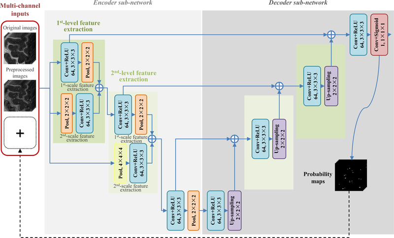
In recent years, deep convolutional neural networks (CNNs) have dominated traditional learning algorithms in various natural and medical image computing tasks, such as image recognition (Krizhevsky et al., 2012; Chan et al., 2015; Simonyan and Zisser- man, 2015; He et al., 2016), semantic segmentation (Noh et al., 2015; Shelhamer et al., 2016; Liu et al., 2017a), anatomical land- mark detection (Zhang et al., 2016, 2017b, 2017c), computer-aided diagnosis/detection (Gao et al., 2015; Shin et al., 2016; Suk et al., 2017; Liu et al., 2017b, 2018), or volumetric image segmentation (Guo et al., 2016; Rajchl et al., 2017; Chen et al., 2017; Kamnitsas et al., 2017; Dou et al., 2017). As the state-of-the-art deep learning models for image segmentation, fully convolutional networks (FCNs) (Shelhamer et al., 2016) can efficiently produce end-to-end segmentation by seamlessly combining global semantic information with local details by using advanced encoder-decoder architectures. However, existing FCN models in the literature (e.g., U-Net (Ronneberger et al., 2015)) usually perform segmentation by using only one source of information (e.g., original images), thus ignoring the fact that the additional guidance from other complementary information sources may be beneficial for improving the segmentation results. To this end, a new multi-channel multi-scale deep convolutional encoder-decoder network (M ² EDN) is proposed in this paper for the task of PVS segmentation. A schematic diagram of the proposed M ² EDN is shown in Fig. 2. As an extension of the original FCNs, the proposed method also applies volumetric operations (i.e., convolution, pooling, and up-sampling) to achieving structured end-to-end prediction. Particularly, it adopts complementary multi-channel inputs to provide both enhanced tubular structural information and detailed image information for precise localization of PVSs. Then, high-level and multi-scale image features are automatically learned to better characterize spatial associations between PVSs and their neighboring brain tissues. Finally, the proposed network is effectively trained from scratch by taking into account the severe imbalance between PVS voxels and background voxels. The output PVS probability map is further used as auxiliary contextual information to refine the whole network for more accurate segmentation of PVSs. Experimental results on 7T brain MR images from 20 subjects demonstrate superior performance of the proposed method, compared with several state-of-the-art methods.

Fig. 2.

The network architecture of the proposed M ² EDN, which consists of an encoder sub-network and a decoder sub-network. The symbol denotes the fusion of feature tensors with identical resolution. Conv: convolution; ReLU: rectified linear unit; Pool: max pooling.

The rest of this paper is organized as follows. In Section 2, previous studies that relate to our work are briefly reviewed. In Section 3.2, both the proposed M ² EDN method and the studied data are introduced. In Section 4, the proposed method is compared with existing PVS segmentation methods, and the role of each specific module of our method is analyzed. In Section 5, we further discuss about the training and generalization of the proposed network, as well as the limitations of its current implementation. Finally, a conclusion of this paper is presented in Section 6.

2. Related work

Available vessel segmentation methods, i.e., learning-based approaches (Ricci and Perfetti, 2007; Marín et al., 2011; Schneider et al., 2015) and filtering methods (Hoover et al., 20 0 0; Xiao et al., 2013; Roychowdhury et al., 2015), are potentially applicable to PVS segmentation. However, direct use of these general methods in the specific task of PVS segmentation is challenging, especially considering that PVSs are very thin tubular structures with various directions and also with lower contrast compared with surrounding tissues (see Fig. 1).

Up to now, only a few automatic/semi-automatic approaches have been developed for PVS segmentation. These approaches can be roughly divided into two categories: (1) unsupervised methods and (2) supervised methods. The unsupervised methods are usually based on simple thresholding, edge detection and/or enhancement, and morphological operations (Frangi et al., 1998; De- scombes et al., 2004; Uchiyama et al., 2008; Wuerfel et al., 2008). For instance, Descombes et al. (2004) applied a region-growing algorithm to initially segment PVSs which were first detected by image filters and then segmented by the Markov chain Monte Carlo method. Uchiyama et al. (2008) used an intensity thresholding method to annotate PVSs in MR images, which were enhanced by a morphological operation. In Wuerfel et al. (2008), an adaptive thresholding method was integrated into a semi-automatic software to delineate PVS structures. Although these unsupervised methods are intuitive, their performance is often limited by manual intermediate steps that are used to heuristically determine the tuning parameters (e.g., thresholds). In particular, these methods do not consider the contextual knowledge on spatial locations of PVSs.

Different from these unsupervised methods, the supervised methods can seamlessly include contextual information to guide the segmentation procedure with carefully-defined image features and/or structured learning strategies. Currently, various supervised learning-based methods have been proposed to segment general vessels. For example, Ricci and Perfetti (2007) adopted a specific line detector to extract features, based on which a support vector machine (SVM) was then trained to segment vessels in retinal images. Schneider et al. (2015) extracted features based on rotation-invariant steerable filters, followed by construction of a random forest (RF) model to segment vessels in the rat visual cortex images. Fraz et al. (2012) used an ensemble classifier trained with orientation analysis-based features to segment retinal vessels. In particular, several supervised learning-based approaches have also been proposed to automatically delineate thin PVS structures in MR images. Park et al. (2016) described local patch appearance using orientation-normalized Haar features. Then, they trained sequential RFs to perform PVS segmentation in an ROI defined based on anatomical brain structures and vesselness filtering (Frangi et al., 1998). Zhang et al. (2017a) first adopted multiple vascular filters to extract complementary vascular features for image voxels in the ROI, and then trained a structured RF (SRF) model to smoothly segment PVSs via a patch-based structured prediction. Although these traditional learning-based methods have shown overall good performance, several limitations still exist: (1) their performance often depends on the hand-crafted features, while such features could be heterogeneous to subsequent classification/regression models and thus may degrade the segmentation performance; (2) the discriminative capacity of hand- crafted features could be hampered by the weak signals of thin PVSs and also by the inherent noise in MR images; (3) a carefully defined ROI is desired (e.g., Park et al., 2016; Zhang et al., 2017a) to ensure effective segmentation, which inevitably increases the complexity in both training and testing, since expertise knowledge is often required to this end.

As the state-of-the-art deep learning models for image segmentation, fully convolutional networks (FCNs) (Shelhamer et al., 2016), e.g., SegNet (Badrinarayanan et al., 2015) and U-Net (Ronneberger et al., 2015), can efficiently produce pixel-wise dense prediction due to their advanced encoder-decoder architectures. Generally, an encoder-decoder architecture consists of a contracting sub-network and a successive expanding sub-network. The encoder part (i.e., contracting sub-network) can capture long-range cue (i.e., global contextual knowledge) by analyzing the whole input images, while the subsequent decoder part (i.e., expanding sub-network) can produce precise end-to-end segmentation by fusing global long-range cue with complementary local details. However, previous FCN-based methods (e.g., U-Net) usually learn a model for segmentation using solely the original images, which ignores critical guidance from other complementary information sources, such as auto-contextual guidance from class confidence (or discriminative probability) maps that are generated by initial networks (trained using the original images) (Tu and Bai, 2010).

Similar to U-Net (Ronneberger et al., 2015) and SegNet (Badrinarayanan et al., 2015), the proposed M ² EDN is also constructed by an encoder sub-network and a decoder sub-network to capture both the global and local information of PVSs in MR images. On the other hand, it additionally owns the following unique properties: (1) Using the combination of different volumetric operation strategies, the complementary multi-scale image features can be automatically learned and fused in the encoder sub-network to comprehensively capture morphological characteristics of PVSs and also spatial associations between PVSs and neighboring brain tissues. (2) Considering that PVSs are the thin tubular structures with weak signals in the noisy MR images, two complementary channels of inputs are initially included in the network. Specifically, using a non-local Haar-transform-based line singularity representation method (Hou et al., 2017), one channel provides the processed T2-weighted MR images with enhanced tubular structural information, but with reduced image details. In parallel, the other channel provides the original noisy T2-weighted MR images with fine local details. (3) Since PVS probability maps generated by the network can naturally provide contextual information of PVSs (Tu and Bai, 2010), we recursively incorporate these maps into the network as an additional input channel to further refine the whole model for achieving more accurate segmentation of PVSs.

3. Materials and method

3.1. Materials

Twenty healthy subjects aged from 25 to 55 were included in this study. The original MR images were acquired with a 7T Siemens scanner (Siemens Healthineers, Erlangen, Germany). Seventeen subjects were acquired using a single channel transmit and 32 channel receive coil (Nova Medical, Wilmington, MA), while the other three subjects were acquired using 8 channel transmit and 32 channel receive coil. The total scan time was around 483 seconds. Both T1- and T2-weighted MR images were scanned for each subject. The T1-weighted MR images were acquired using the MPRAGE sequence (Mugler and Brookeman, 1990) with the spatial resolution of 0. 65 × 0. 65 × 0. 65 mm ³ or 0. 9 × 0. 9 × 1. 0 mm ³, while the T2-weighted MR images were acquired using the 3D variable flip angle turbo-spin echo sequence (Busse et al., 2006) with the spatial resolution of 0. 5 × 0. 5 × 0. 5 mm ³ or 0. 4 × 0. 4 × 0. 4 mm ³. The reconstructed images had the same voxel sizes as those acquired images, and no interpolation was applied during image re-construction.

The T2-weighted MR images for all studied subjects are used to segment PVSs, as PVSs are usually more visible in T2-weighted MR images (Hernández et al., 2013). The ground-truth segmentation was defined cooperatively by an MR imaging physicist and a computer scientist specialized in medical image analysis. Since manual annotation is a highly time-consuming task, the whole brain PVS masks were created just for 6 subjects, while the right hemisphere PVS masks were created for all the remaining 14 subjects. More detailed information about the studied data can be found in Zong et al. (2016).

3.2. Method

In this part, the proposed multi-channel multi-scale encoder-decoder network (M ² EDN) is introduced in detail. First, we describe the overall network architecture, followed by introduction of each key module one-by-one. Then, we discuss the training and testing procedures, including some specific operations to mitigate severe imbalanced learning issue in our task of PVS segmentation.

3.2.1. Network architecture

As shown in Fig. 2, the proposed M ² EDN is a variant FCN model (Shelhamer et al., 2016) that consists of multiple convolutional layers, pooling layers, and up-sampling layers. Specifically, it includes an encoder sub-network and a decoder sub-network. In the encoder sub-network, the blue blocks first perform 64 channels of 3 × 3 × 3 convolution with the stride of 1 and zero padding, and then calculate the rectified linear unit (ReLU) activations (Krizhevsky et al., 2012). Besides, the orange blocks per- form 2 × 2 × 2 max pooling with the stride of 2, while the yellow block performs 4 × 4 × 4 max pooling with the stride of 4. It can be observed that the network inputs are down-sampled three times in this encoder sub-network, i.e., the included convolutional and pooling operations are arranged and orderly executed at three de- creasing resolution levels. In this way, we attempt to comprehensively capture the global contextual information of PVSs by using the combination of different volumetric operation strategies.

Symmetric to the encoder sub-network, the subsequent de-coder sub-network consists of operations arranged at three increasing resolution levels. The blue blocks in this sub-network perform the same convolutional processing as those in the encoder sub-network, while the followed purple blocks up-sample the obtained feature maps using 2 × 2 × 2 kernels with the stride of 2. At each resolution level, a skip connection is included to fuse the up-sampled feature maps with the same level feature maps obtained from the previous encoder sub-network, in order to complementarily combine global contextual information with spatial details for precise detection and localization of PVSs. The final magenta block performs 1 × 1 × 1 convolution and sigmoid activation to calculate voxel-wise PVS probability maps from high-dimensional feature maps.

Both the encoder sub-network and the decoder sub-network contain the combination operations (i.e., the symbol ⊕ in Fig. 2) for the fusion of feature tensors with equal resolution. Multiple alternatives can be applied to this step, e.g., the voxel-wise addition, voxel-wise averaging, and tensor concatenation. Similar to that in U-Net (Ronneberger et al., 2015), the concatenation operation is adopted in this paper as it shows overall best performance. The coefficients of the network shown in Fig. 2 can be learned using the training images with ground-truth segmentations of PVSs.

3.2.2. Multi-channel inputs

As illustrated in Fig. 2, the proposed M ² EDN has two complementary input channels. That is, one channel loads the preprocessed T2-weighted MR images with high-contrast tubular structural information, and another channel loads the original T2-weighted MR images for providing image details that are obscured during the preprocessing procedure (i.e., for image enhancement and denoising).

A non-local image filtering method (i.e., BM4D, Maggioni et al., 2013) and its variant with Haar-transformation-based line singularity representation (Hou et al., 2017) are adopted to remove noise and enhance the thin tubular structures, respectively. More specifically, each original T2-weighted MR image is divided into multiple reference cubes with the size of S × S × S. The Haar transformation is then performed on a group of K nonlocal cubes within a small neighborhood (i.e., 3 × 3 × 3) of the center of each reference cube, based on which the tubular structural information can be effectively represented in the transformed sub-bands. The transformation coefficients are then nonlinearly mapped to enhance signals relevant to PVSs. Given the transformation coefficients after processing, the enhanced reference cubes are then reconstructed by the inverse Haar transformation, which are finally aggregated together as the enhanced T2-weighted MR image. Finally, the enhanced T2-weighted MR image is further processed by the BM4D method to suppress the remaining noise.

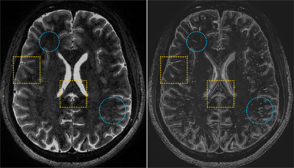
Fig. 3 shows an example of axial T2-weighted MR slice (i.e., at the left-panel), as well as the enhanced and denoised counterpart (i.e., at the right-panel). We can observe that the tubular structures are effectively enhanced in the preprocessed images (e.g., in the blue circles), while sacrificing some image details (e.g., in the yellow boxes). In our experiments, two parameters S and K used in the nonlocal image enhancement were set as 7 and 8, respectively. More information regarding this non-local image enhancement method can be found in Hou et al. (2017).

Fig. 3.

An example of the original T2-weighted MR image (at the left-panel) and the processed image (at the right-panel) shown in the axial view. The blue circles present the effectively enhanced tubular structures via the method proposed in Hou et al. (2017), while the yellow boxes show the lost image information, due to the enhancement and denoising procedures. (For interpretation of the references to color in this figure legend, the reader is referred to the web version of this article.)

3.2.3. Multi-scale feature learning

To robustly quantify the structural information of PVSs and adjacent brain tissues, the proposed M ² EDN is designed to learn multi-scale features in the encoder sub-network.

As shown in Fig. 2, at the first two decreasing resolution levels (i.e., the 1st-level and the 2nd-level feature extraction), besides the commonly used modules of convolution plus pooling, the input images are simultaneously down-sampled first, followed by executing of convolutional operations on the down-sampled images. Specifically, the input images are simply half-sized using 2 × 2 × 2 max pooling with the stride of 2 at the 1st-level feature extraction, while quarter-sized using 4 × 4 × 4 max pooling with the stride of 4 at the 2nd-level feature extraction. In this way, different scales of features at each resolution level can be efficiently quantified in parallel, which are then fused as the input to the subsequent resolution level. It is also worth noting that this operation is not applied to the last decreasing resolution, mainly considering that PVSs are the thin tubular structures which could be invisible after one-eighth down-sampling.

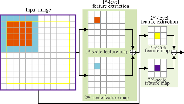
An illustration of the above procedure for a 2D input image (with the size of 12 × 12) is shown in Fig. 4, where multi-scale features are hierarchically learned at two successive feature extraction stages. At each stage, two different scales of feature representations are extracted for the input image. For instance, for the 1st- level feature extraction, the orange pixel in the 1st-scale feature map (top) is generated by performing 3 × 3 convolution followed by 2 × 2 max pooling on the 4 × 4 orange region in the input image, while the corresponding blue pixel in the 2nd-scale feature map (bottom) is generated by performing 2 × 2 max pooling followed by 3 × 3 convolution on the 6 × 6 blue region in the input image. Similarly, for the 2nd-level feature extraction, the yellow and purple pixels in the 1st-scale and 2nd-scale feature maps correspond, respectively, to the 10 × 10 yellow region and the 12 × 12 purple region in the input image. Note that the 2nd-scale feature map (bottom) for the 2nd-level feature extraction is generated by directly performing 4 × 4 max pooling followed by 3 × 3 convolution on the input image, while the corresponding 1st-scale feature map (top) is obtained by performing 3 × 3 convolution followed by 2 × 2 max pooling on feature maps that are produced by the 1st-level feature extraction. Based on the above operations, at each feature extraction stage, two complementary feature maps are extracted from the identical center regions to characterize the input in a fine scale (i.e., 4 × 4) and a coarse scale (i.e., 6 × 6), respectively.

Fig. 4.

An illustration of multi-scale feature learning for a 2D input image (with the size of 12 × 12) in the proposed encoder sub-network. For the 1st-level feature extraction, the orange pixel in the 1st-scale feature map (top) and the blue pixel in the 2nd-scale feature map (bottom) correspond to the 4 × 4 orange region and the 6 × 6 blue region in the input image, respectively. Similarly, for the 2nd-level feature extraction, the yellow and purple pixels in the 1st- and 2nd-scale feature maps correspond to the 10 × 10 yellow region and the 12 × 12 purple region in the input image, respectively. That is, at each feature extraction stage, two complementarily feature maps are extracted from the identical center regions to characterize the input in both a fine scale (i.e., 4 × 4) and a coarse scale (i.e., 6 × 6). (For interpretation of the references to color in this figure legend, the reader is referred to the web version of this article.)

3.2.4. Auto-contextual information

The strategy of auto-context was first introduced by Tu and Bai (2010), which was then successfully applied to various tasks of medical image analysis (e.g., Wang et al., 2015; Chen et al., 2017), showing remarkable performance. The general idea is to adopt both the original image and the class confidence (or discriminative probability) maps generated by a classifier (trained using the original images) for recursively learning an updated classifier to refine the output probability map. This procedure can be repeated multiple times until convergence to yield sequential classification models. Thus, high-level contextual information can be effectively combined with low-level image appearance iteratively to improve the learning performance.

Inspired by the idea of this auto-context model (Tu and Bai, 2010), we first train an initial M ² EDN model using multi-channel input images (i.e., the original and preprocessed T2- weighted MR images) as the low-level image appearance information. Then, besides the two original input channels, the PVS probability maps produced by this initial M ² EDN are also included as third input channel (i.e., indicated by a black dotted arrow line in Fig. 2) to provide complementary contextual information. This kind of high-level contextual guidance could provide implicit shape information to assist the learning of image features in each convolutional layer, which could facilitate the training and updating of our network for further improving the segmentation results.

3.2.5. Imbalanced learning

In our segmentation task, there exists a severe class-imbalance issue, where the number of voxels in the PVS regions (i.e., positive observations) is much smaller than that in the background (i.e., negative observations). This real-world challenge hampers the stability of most standard learning algorithms, since conventional methods usually assume balanced distributions or equal misclassification costs (i.e., using simple average error rate) across different classes. To deal with this class-imbalance problem, two widely-used strategies have been proposed in the literature (He and Garcia, 2009; Liu et al., 2014; Lian et al., 2016), i.e., (1) data rebalancing, and (2) cost-sensitive learning. In this study, we adopt these two strategies in the training phase to ensure the effectiveness of our network in identifying the minority PVS voxels from the background.

In consideration of the generalization capacity of the proposed M ² EDN, the diversity of selected training samples is also taken into account during the data rebalancing procedure. More specifically, training sub-images in each mini-batch are generated on-the-fly by cropping equal-sized volumetric chunks, both randomly from the whole image and randomly from the dense PVS regions within the image. In this way, training samples in each epoch not only are diversified but also contain a considerable amount of voxels belonging to the PVSs. Moreover, the training data is in some sense implicitly augmented due to this operation, because a large number of sub-images with partial differences can be randomly sampled from a single MR image.

It is worth noting that a sub-image generated by the above procedure is likely to contain more background voxels than PVS voxels, even we sample densely from PVS regions. To address this is- sue, we further design a cost-sensitive loss function based on F-measure for training the proposed network. Let $Y={\left\{y_i\right\}}_{i=1}^N$ be the ground-truth segmentation for a sub-image consisting of N voxels, where y _i = 1 denotes that the i th voxel belongs to the PVSs, while y i = 0 the background. Accordingly, we assume $\widehat{Y}={\left\{{\widehat{y}}_i\right\}}_{i=1}^N$ is the PVS probability map produced by the proposed M²EDN, where ${\widehat{y}}_i\in [0,1]$ and i = 1, ..., N. Then, the loss function L _F used in our network can be represented as

$$L_F=1-\frac{\left(1+{\beta }^2\right){\sum }_{i=1}^N{y}_i{\widehat{y}}_i+ϵ}{{\beta }^2{\sum }_{i=1}^N{y}_i+{\sum }_{i=1}^N{\widehat{y}}_i+ϵ},$$ (1)

where ϵ is a small scalar (e.g., 1e-5) to ensure numerical stability for calculating the loss value. The tuning parameter β > 0 determines if precision (i.e., positive prediction value) contributes more than recall (i.e., true positive rate or sensitivity) during the training procedure, or conversely. We empirically set β= 1, which means precision and recall have equal importance in the task of PVS segmentation.

3.2.6. Implementations

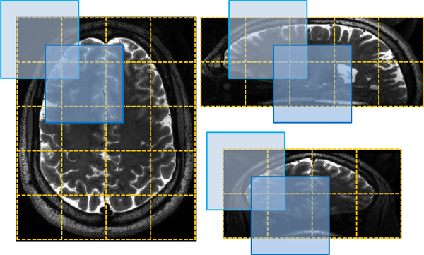
The proposed networks were implemented using Python based on the Keras package (Chollet, 2015), and the computer we used contains a single GPU (i.e., NVIDIA GTX TITAN 12GB). Training images were flipped in the axial plane to augment the available training sub-images as well as increase their diversity for better generalization of trained networks. Using the procedure described in Section 3.2.5, the size of each training sub-image was 96 × 96 × 96, and the size of a mini-batch in each epoch was 2. The network was trained by the Adam optimizer using recommended parameters. In the testing phase, considering FCNs desire large inputs to provide rich semantic information, each testing image was divided into 168 × 168 × 168 sub-images that are overlapped with each other. After prediction, we only kept segmentation results for the non-overlapped 96 × 96 × 96 central chunks in the overlapped 168 × 168 × 168 testing sub-images. Finally, the non-overlapped central chunks were padded together as the out-put with equal size to the original testing image. A 2D illustration of generating the testing sub-images is presented in Fig. 5. Our experiments empirically show that the method keeping only the non-overlapped central chunks for the final segmentation performs relatively better than the method preserving also the overlapped boundaries. It may be because the prediction for the boundaries is less accurate than that for the central parts, considering that the convolutional layers contain zero-padding operations.

Fig. 5.

A 2D illustration from three different views to describe the procedure of generating the testing sub-images. The input image is divided into multiple blue blocks that are overlapped with each other. After prediction, only their central chunks with yellow dotted boundaries are padded together as the final segmentation of the input image. (For interpretation of the references to color in this figure legend, the reader is referred to the web version of this article.)

4. Experiments and analyses

In this section, we first present the experimental settings and the competing methods, and then compare the segmentation results achieved by different methods. In addition, we verify the effectiveness of each key module of the proposed M ² EDN via evaluating their influence on the segmentation performance.

4.1. Experimental settings

Following the experimental settings in Park et al. (2016), six subjects with whole-brain ground-truth masks were used as the training samples, while the remaining fourteen subjects with right- hemisphere ground-truth masks were used as the testing samples.

Using manual annotations as the reference, the segmentation performance of our method was quantified and compared with that of other methods using three metrics, i.e., (1) the Dice similarity coefficient (DSC), (2) the sensitivity (SEN), and (3) the positive prediction value (PPV), defined as

$$\text{DSC}=\frac{2\text{TP}}{2\text{TP}+\text{FP}+\text{FN}};$$ (2)

$$\text{SEN}=\frac{\text{TP}}{\text{TP}+\text{FN}};$$ (3)

$$\text{PPV}=\frac{\text{TP}}{\text{TP}+\text{FP}},$$ (4)

where TP (i.e., true positive) denotes the number of predicted PVS voxels inside the ground-truth PVS segmentation; scalar FP (i.e., false positive) denotes the number of predicted PVS voxels out-side the ground-truth PVS segmentation; scalar TN (i.e., true negative) represents the number of predicted background voxels out-side the ground-truth PVS segmentation; scalar FN (i.e., false negative) represents the number of predicted background voxels inside the ground-truth PVS segmentation.

4.2. Competing methods

We first compared our proposed M ² EDN method with a base- line method, i.e., a thresholding method based on Frangi’s vesselness filtering (FT) (Frangi et al., 1998). Then, we also compared M ² EDN with two state-of-the-art methods, including (1) a traditional learning-based method, i.e., structured random forest (SRF) (Zhang et al., 2017a), and (2) the original U-Net architecture (Ronneberger et al., 2015). These three competing methods are briefly introduced as follows.

1. Frangi’s vesselness filtering (FT) (Frangi et al., 1998): The Frangi’s vesselness filtering method proposed in Frangi et al. (1998) is a thresholding method. Considering that PVSs mainly spread in the white matter (WM) region (Zong et al., 2016), the WM tissue in T2-weighted MR image should be extracted first as ROI for reliable vessel detection. Then, all possible thin tubular structures in the ROI were detected using Frangi’s filter (Frangi et al., 1998) to generate a vesselness map. Finally, voxels in the ROI with higher vesselness than a certain threshold were determined as the PVS voxels. Several vesselness thresholds were tested, and the optimal thresholds were obtained for different subjects. More details with respect to the segmentation of WM, the definition of ROI, and the vesselness thresholding can be found in Park et al. (2016) and Zhang et al. (2017a). To summarize, FT does not need any label information, and thus is an unsupervised method.

2. Structured random forest (SRF) (Zhang et al., 2017a): The structured random forest model using vascular features was implemented to smoothly annotate PVSs. More specifically, the ROI for PVS segmentation was defined similarly as that for the FT method. Then, for each voxel sampled from the ROI via an entropy-based sampling strategy (Zhang et al., 2017a), three different types of vascular features based on three filters (i.e., steerable filter (Freeman et al., 1991), Frangi’s vesselness filter (Frangi et al., 1998), and optimally oriented flux (Law and Chung, 2008)) and the corresponding cubic label patches were extracted to train a SRF model (with 10 independent trees, each having the depth of 20). That is, the SRF method is a supervised method, requiring label information for training image patches.

3. U-Net (Ronneberger et al., 2015): It should be noted that the original U-Net is a simplified version of the proposed M ² EDN, without using multi-channel inputs and multi-scale feature learning. For fair comparison, the two learning strategies (i.e., data resampling, and cost-sensitive learning) introduced in Section 3.2.5 to deal with class-imbalanced problem were also applied to the U-Net. Besides, U-Net and our proposed M ² EDN share the same size of sub-images in both the training and testing procedures.

4.3. Result comparison

The quantitative segmentation results obtained by our M ² EDN method and the three competing methods, on both the train- ing and testing images, are reported in Tables 1 and 2. From Tables 1 and 2, we have the following observations. First, com- pared with the conventional unsupervised method (i.e., FT) and supervised method (i.e., SRF), two deep learning-based methods (i.e., U-Net, and our M ² EDN method) achieve better results in PVS segmentation in terms of three evaluation criteria (i.e., DSC, SEN, and PPV). This implies that incorporating feature extraction and model learning into a unified framework, as we did in M ² EDN, does improve the segmentation performance. The possible rea- son could be that the task-oriented features automatically learned from data are consistent with the subsequent classification model, while the hand-crafted features used in SRF are extracted independently from the model learning. Second, the proposed M ² EDN out- performs the original U-Net, mainly due to the use of three key modules in the proposed method, i.e., the complementary multi-channel inputs, the multi-scale feature learning strategy, and the auto-contextual information provided by the initial PVS probability maps. In particular, the proposed M ² EDN method usually achieves superior SEN values in most cases, suggesting that our method can effectively identify PVS regions from those large amounts of back- ground regions. Moreover, by comparing results on the training images (i.e., Table 1) with those on the testing images (i.e., Table 2), we can also find that the proposed M ² EDN generalizes well in this experiment.

Table 1.

The average (±standard deviation) performance, in terms of DSC, SEN, and PPV, obtained by different methods on the training set.

	FT	SRF	U-Net	M 2 EDN
DSC	0.51 ±0.05	0.68 ±0.03	0.70 ±0.07	0.77 ±0.04
SEN	0.54 ±0.16	0.66 ±0.05	0.64 ±0.14	0.73 ±0.11
PPV	0.56 ±0.12	0.71 ±0.03	0.81 ±0.07	0.84 ±0.07

Table 2.

The average (±standard deviation) performance, in terms of DSC, SEN, and PPV, obtained by different methods on the testing set.

	FT	SRF	U-Net	M 2 EDN
DSC	0.53 ±0.08	0.67 ±0.03	0.72 ±0.05	0.77 ±0.06
SEN	0.51 ±0.10	0.65 ±0.04	0.77 ±0.08	0.74 ±0.12
PPV	0.62 ±0.08	0.68 ±0.04	0.70 ±0.10	0.83 ±0.05

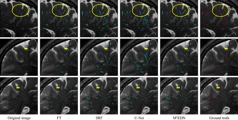
The corresponding qualitative comparison is presented in Fig. 6. As can be seen, the automatic segmentations obtained by the pro- posed M ² EDN are more consistent with the manual ground truth in these examples, especially for the relatively low-contrast PVSs indicated by the yellow arrows and ellipses.

Fig. 6.

Illustration of PVS segmentation achieved by four different methods, with each row denoting a specific subject. The first column and the last column denote, respectively, the original images and the ground truth annotated by experts. The yellow ellipses and arrows indicate low-contrast PVSs that can be still effectively detected by the proposed method. (For interpretation of the references to color in this figure legend, the reader is referred to the web version of this article.)

4.4. Module analyses

In this subsection, we evaluate the effectiveness of each key module of the proposed M ² EDN via assessing their influence on the segmentation performance.

4.4.1. Role of multi-channel inputs

To assess the effectiveness of multi-channel inputs, we removed one source of input images, and then trained the mono-channel networks in the same way as that for the multi-channel network. Specifically, the quantitative results produced by our method using only the original images (denoted as M ² EDN-O), only the pre- processed images (denoted as M ² EDN-P), and the multi-channel inputs (i.e., M ² EDN using both the original and preprocessed images) are compared in Table 3. It can be found from Table 3 that both M ² EDN-O (using solely the original images) and M ² EDN-P (using solely the preprocessed images) obtain similar overall accuracy (i.e., DSC), where the former one and the latter one lead to better SEN and PPV, respectively. On the other hand, M ² EDN using both the original and the preprocessed images further improves the performance, by effectively combining the complementary information provided by the two different channels during the learning procedure.

Table 3.

The average (±standard deviation) testing performance, in terms of DSC, SEN, and PPV, obtained by the mono-channel and multi-channel M ² EDN. M ² EDN-O and M ² EDN-P denote, respectively, the mono-channel M ² EDN using solely the original images and solely the prepro- cessed images.

	M 2 EDN-O	M 2 EDN-P	M 2 EDN
DSC	0.73 ±0.04	0.72 ±0.09	0.77 ±0.06
SEN	0.78 ±0.09	0.67 ±0.14	0.74 ±0.12
PPV	0.71 ±0.10	0.81 ±0.06	0.83 ±0.05

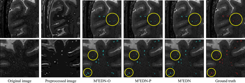
Two example images segmented via M ² EDN-O, M ² EDN-P, and M ² EDN are visualized in Fig. 7, which are consistent with the quantitative results shown in Table 3. From the results presented in Table 3 and Fig. 7, we can observe that combining the original image with the preprocessed image can effectively improve the automatic annotation, compared with the case of using only one in- put image only, e.g., for the regions marked by the yellow circles in Fig. 7.

Fig. 7.

Illustration of segmentations obtained by the mono-channel network using the original image (i.e., M ² EDN-O), the mono-channel network using the preprocessed image (i.e., M ² EDN-P), and the multi-channel network (i.e., M ² EDN). The yellow circles indicate improved segmentations due to the use of complementary multi-channel inputs. (For interpretation of the references to color in this figure legend, the reader is referred to the web version of this article.)

4.4.2. Role of multi-scale features

As one main contribution of this paper, the proposed M ² EDN method extends the original U-Net by including the complementary coarse-scale feature extraction steps (i.e., the 2nd-scale feature extraction as shown in Fig. 2) in the encoder sub-network. To demonstrate its effectiveness, we removed the 2nd-scale feature extraction from the network to form a mono-scale version of the proposed M ² EDN (denoted as M ² EDN-S). Then, we further increased the depth of M ² EDN-S (by adding additional pooling, convolutional, and up-sampling layer) to ensure that its network complexity is comparable to that of M ² EDN. The architecture of M ² EDN-S can be found in Fig. S1 of the Supplementary Materials. We should note that M ² EDN-S is still different from the original U-Net, since multi-channel inputs are used in M ² EDN-S. Using the same experimental settings, the testing results obtained by M ² EDN-S are compared with those by M ² EDN in Table 4. As can be seen, the multi-scale feature learning procedure effectively improves the overall segmentation performance, especially in terms of SEN and PPV, which means that false positive and false negative detections are partially reduced.

Table 4.

The average (±standard deviation) performance, in terms of DSC, SEN, and PPV, obtained by the mono-scale feature learning strategy (i.e., M ² EDN-S) and multi-scale feature learning strategy (i.e., M ² EDN) for the eleven testing images.

	M 2 EDN-S	M 2 EDN
DSC	0.74 ±0.08	0.77 ±0.06
SEN	0.70 ±0.13	0.74 ±0.12
PPV	0.81 ±0.06	0.83 ±0.05

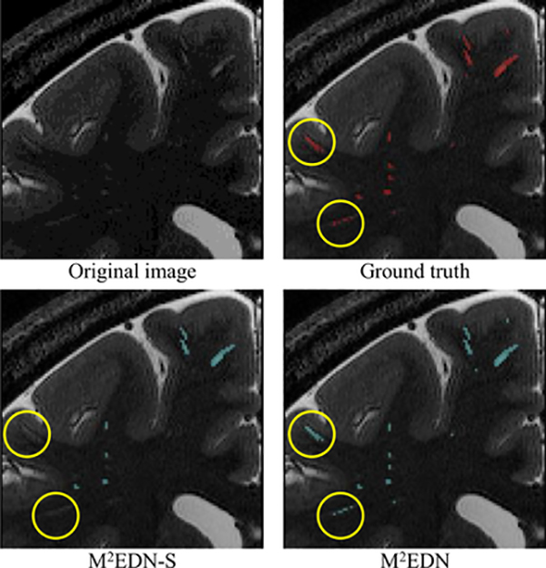
As a qualitative illustration, two automatic segmentations produced, respectively, by M ² EDN-S and M ² EDN are visually compared in Fig. 8. Regarding the manual annotation as the reference,we can observe that M ² EDN leads to more accurate segmentation than M ² EDN-S. For instance, the multi-scale feature learning strategy effectively removed false negative detections marked by the yellow circles.

Fig. 8.

Illustration of segmentations obtained by the proposed method with mono-scale feature learning (i.e., M ² EDN-S) and multi-scale feature learning (i.e., M ² EDN), respectively. The yellow circles indicate that the multi-scale feature learning strategy can effectively remove false positive detections produced by M ² EDN-S. (For interpretation of the references to color in this figure legend, the reader is referred to the web version of this article.)

It is also worth noting that multi-scale feature learning is beneficial for the original U-Net as well, even when we use only the mono-channel input to train the network. Specifically, M ² EDN-O introduced in Section 4.4.1 is actually a variant of U-Net using the proposed multi-scale feature learning strategy. By comparing the results achieved by M ² EDN-O shown in Table 3 with those achieved by the original U-Net shown in Table 2, we can observe that the proposed multi-scale feature learning strategy does improve the segmentation performance of the original U-Net (i.e., average DSC is increased from 0.72 to 0.73).

Similarly, we can regard M ² EDN-S as a variant of U-Net that uses multi-channel inputs. By comparing the results obtained by M ² EDN-S shown in Table 4 with those obtained by the original U-Net shown in Table 2, we can observe that the multi-channel inputs are also beneficial for the original U-Net (i.e., average DSC is improved from 0.72 to 0.74). This observation is consistent with the results shown in Table 3 and thus supports our previous discussion in Section 4.4.1.

4.4.3. Role of auto-contextual information

In the proposed method, our empirical studies show that learning sequential networks in multiple iterations brings few improvements with relatively large price. To this end, the auto-contextual information was used only once in our experiment, i.e., the initial network was trained using the multi-channel inputs of the original and preprocessed T2-weighted MR images, and then the output probability maps were combined with the input images to train the subsequent network as the final M ² EDN model.

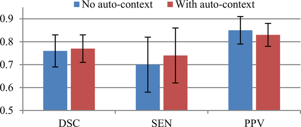
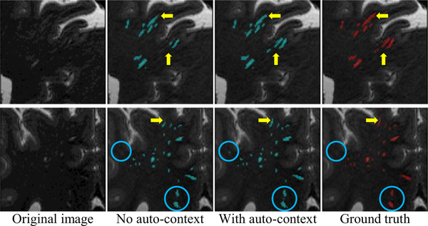
The quantitative testing results obtained by the networks trained with and without the auto-contextual information are compared in Fig. 9. It can be seen that the use of auto-context strategy further refines the average DSC (from 0.76 ± 0.07 to 0.77 ± 0.06). More specifically, it makes an adjustment or a compromise between SEN (from 0.70 ± 0.12 to 0.74 ± 0.12) and PPV (from 0.85 ± 0.06 to 0.83 ± 0.05), to improve the overall segmentation performance. Implicitly, the role of the auto-context strategy can be interpreted as to improve the output segmentations globally by enhancing the input probability maps (i.e., improving true positive detections), though it may bring additional false positives to some extent.

Fig. 9.

The average (± standard deviation) testing performance, in terms of DSC, SEN, and PPV, obtained by the proposed method with or without auto-context information.

As an example, two qualitative illustrations obtained by the proposed method with and without the auto-contextual information are shown in Fig. 10, where the yellow arrows and the blue circles indicate the refined PVS annotations and additional false positives, respectively. We can notice that multiple PVSs with relatively low contrast are detected by adding auto-contextual information (indicated by yellow arrows), while few false positive detections (indicated by blue circles) are included simultaneously. Overall, the use of auto-context strategy can improve the segmentation based on the contextual information provided by the probability maps.

Fig. 10.

Illustration of segmentations obtained by the proposed M ² EDN with or without auto-context information. The yellow arrows and the blue circles indicate, respectively, the refined PVS annotations and additional false positives, both due to the use of auto-context strategy. (For interpretation of the references to color in this figure legend, the reader is referred to the web version of this article.)

4.4.4. Role of balanced data sampling

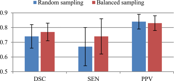
The proposed method adopts a balanced data sampling strategy and an F-measure-based loss function to mitigate the influence of class-imbalance challenge on PVS segmentation. As an example to verify its effectiveness, we performed another experiment to train our network using sub-images generated on-the-fly by randomly cropping overlapped chunks from the whole image. Using 6 sub- jects with the whole-brain ground truth for training while using the remaining subjects for testing, the quantitative testing results obtained by this random sampling strategy was compared with those obtained by the balanced sampling strategy. Based on the results presented in Fig. 11, we can observe that the balanced data sampling leads to much better quantitative performance, especially higher SEN (from 0.67 ± 0.13 to 0.74 ± 0.12 ), i.e., less false negatives, than the general random sampling, which reflects the effectiveness of the employed data sampling strategy.

Fig. 11.

The average (± standard deviation) testing performance (in terms of DSC, SEN, and PPV) obtained, respectively, by a random sampling strategy and the pro- posed balanced sampling strategy.

5. Discussions

In this section, we present some discussions about the robustness and generalization of the proposed method. As a part of our study in the future, we also indicate some limitations and open rooms for the current method.

5.1. Network training and generalization

Multiple operations were adopted in this paper to ensure effective training of deep neural networks from relatively small-sized data with severe class-imbalance issue. Specifically, an F-measure-based cost-sensitive loss was used together with a balanced data sampling strategy to deal with the class-imbalance issue. The data sampling strategy could also partly mitigate the challenge caused by small-sized data, since a large amount of training sub-images with considerable diversities can be generated from a single image or the corresponding axial-plane-flipped image. The outputs of the initial network were further used as an additional input channel for the training of an updated network, considering they can provide auto-contextual information to guide the training process to obtain a more accurate segmentation model. The quantitative evaluation presented in Fig. 11 has demonstrated that the class-imbalance issue was effectively limited by the imbalanced- learning strategies. The comparison between the experimental results in the last column of Tables 1 and 2 has shown that, overall, the trained networks can be generalized well, as comparable segmentation performance can be obtained on both the training and testing subjects. Also, the evaluation presented in Fig. 9 has shown that the auto-context strategy can help to refine the final segmentation. To further verify the generalization of our trained networks, we performed additional evaluations as follows.

First, using 6 subjects with whole-brain ground truth as the training set, we divided the remaining 14 subjects as two testing groups by checking if their scanning coils were the same as those of the training set. The quantitative segmentation results obtained by U-Net, M ² EDN-O, M ² EDN-P, M ² EDN-S, and M ² EDN on the two testing groups are then compared in Fig. 12 (a). We can find that the proposed M ² EDN has better performance than its variants (i.e., M ² EDN-O, M ² EDN-P, and M ² EDN-S) and U-Net on both testing groups. In addition, although the proposed method has better segmentation accuracy on the testing images acquired using the same coil as the training images, the difference between the two testing groups is not large.

Fig. 12.

(a) The quantitative segmentation performance (in terms of DSC) for the testing images acquired using the coils identical to or different from the training images.(b) The quantitative testing results (in terms of DSC) obtained by the networks trained using, respectively, the images with whole-brain ground truth and the images with right-hemisphere ground truth.

Second, we reversed the data partition to train the networks using 14 subjects that have only right-hemisphere ground truth, and then evaluated the trained networks on 6 testing subjects with whole-brain ground truth. It is worth noting that this task is relatively challenging, since the training set does not contain sub- images from the left hemisphere. In Fig. 12 (b), the segmentation performance of the proposed M ² EDN is compared with that of U- Net, M ² EDN-O, M ² EDN-P, and M ² EDN-S. It can be found that the proposed method still outperforms the original U-Net architecture. In addition, the multi-channel inputs and the multi-scale feature learning are still beneficial for the proposed method, as M ² EDN has better performance than its variants (i.e., M ² EDN-O, M ² EDN-P, and M ² EDN-S). On the other hand, we should also note that M ² EDN trained on the whole brain images has better performance than that trained on the right hemisphere images. This is intuitive and reasonable, given the fact that more comprehensive data has been used for training the network in the former case.

The above discussions and evaluations demonstrate that the proposed M ² EDN generalized relatively well in our experiments. In addition, it also indicates that, including more training images with wide range of diversity is expected for further improving the performance of the proposed M ² EDN.

5.2. Network architecture

Fully convolutional networks, e.g., U-Net, greatly improve the accuracy of automatic image segmentation, mainly due to task-oriented feature learning, encoder-decoder architectures, and seamless fusion of semantic and local information. For example, the quantitative experimental results presented in Table 2 have shown that U-Net and the proposed M ² EDN can produce more accurate segmentation of PVSs than the traditional learning-based methods. Our M ² EDN extended U-Net by including multi-channel inputs and multi-scale feature learning. The analyses presented in Sections 4.4.1 and 4.4.2 have demonstrated that these modifications to the original U-Net architecture are beneficial, as more comprehensive information regarding PVS and surrounding brain tissues can be extracted to guide the training of an effective segmentation network.

Multiple operations have also been used in the literature to re- fine the final segmentations produced by deep neural networks. For example, in Kamnitsas et al. (2017), a fully connected conditional random field (CRF) was concatenated with multi-scale CNN for segmentation of brain lesions. In Chen et al. (2017), the auto-context strategy was used to develop sequential residual networks for segmentation of brain tissues. Inspired by the auto-context model (Tu and Bai, 2010) and similar to Chen et al. (2017), our M ² EDN implemented two cascaded networks, where the outputs of the initial network were used as high-level contextual knowledge to train an updated network for more accurate PVS segmentation. It is worth noting that, using auto-context and using CRF to refine deep neural networks are distinct in principle. The former strategy updates directly the parameters of trained networks, which means the image features learned by the intermediate layers are further refined with respect to the high-level contextual guidance. However, the latter strategy refines solely the output segmentation, which is independent of the updating of trained networks.

5.3. Limitations of current method

While the proposed M ² EDN obtained competitive segmentation accuracy compared with the state-of-the-art methods, there are still some rooms for further improvement.

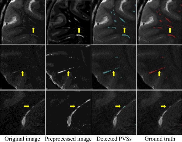
Fig. 13 presents some typical failed segmentations. (1) The pro- posed method may fail to detect PVSs with very low contrast (compared with the adjacent brain tissues), especially when the weak PVSs were not effectively enhanced or even removed in the preprocessed image (e.g., the first row in Fig. 13). One direct way to overcome such difficulty is to adaptively determine the parameters for the tubular structure enhancement method (Hou et al., 2017) to pay more attention to these weak PVSs. (2) The proposed method may fail to completely detect thick PVSs with inhomogeneous intensities along the penetrating direction (e.g., the second row in Fig. 13). Potentially, we may need to find an appropriate way to include some connectivity constraints to guide the training of our network. (3) Sometimes the proposed method may produce some false positive detections, e.g., the false recognition of a separate ventricle part as PVS in the last row of Fig. 13. To reduce such kind of false positives, including accurate white matter mask to refine the segmentation is needed, considering that PVSs largely exist in the white matter.

Fig. 13.

Illustration of typical failed segmentations produced by the proposed method. The failed segmentations are indicated by yellow arrows. (For interpretation of the references to color in this figure legend, the reader is referred to the web version of this article.)

While the auto-context strategy could provide high-level contextual guidance to refine the final segmentation, it inevitably in- creased the training and testing complexity, as the input images should go through at least two cascaded networks. An alternative way to more efficiently improve the final segmentation is to localize and focus more on “hard to segment” voxels during the iterative training of a single network. In other words, the data sampling strategy may be adjusted along the training process to extract more training sub-images from “hard to segment” regions.

6. Conclusion

In this study, we have proposed a multi-channel multi-scale encoder-decoder network (M ² EDN) to automatically delineate PVSs in 7T MR images. The proposed method can perform an efficient end-to-end segmentation of PVSs. It adopts the complementary multi-channel inputs as well as multi-scale feature learning strategy to comprehensively characterize the structural information of PVSs. The auto-context strategy is also used to provide additional contextual guidance for further refining the segmentation results. The experimental results have shown that the proposed method is superior to several state-of-the-arts. Moreover, the proposed M ² EDN method can be further improved in the future from multiple aspects, e.g., (1) it will be valuable to include vesselness maps and connectivity constraints into the network to provide additional guidance for further reducing the false negative predictions; (2) it will be meaningful to further extend the current multi-scale feature learning strategy to enrich the scales of learned features for more comprehensive characterization of the structural information of PVSs; (3) it is desirable to collect more subjects with 7T MR images to further verify the performance of the proposed method, as well as to develop deeper and more discriminative networks for PVS segmentation.

References

- Badrinarayanan V, Kendall A, Cipolla R, 2017. SegNet: A deep convolutional encoder-decoder architecture for image segmentation. Image Segmentation, IEEE Trans. Pattern Anal. Mach. Intel 39 (12), 24 81–2495. [DOI] [PubMed] [Google Scholar]
- Busse RF, Hariharan H, Vu A, Brittain JH, 2006. Fast spin echo sequences with very long echo trains: design of variable refocusing flip angle schedules and generation of clinical T2 contrast. Magn. Reson. Med 55 (5), 1030–1037. [DOI] [PubMed] [Google Scholar]
- Chan T-H, Jia K, Gao S, Lu J, Zeng Z, Ma Y, 2015. PCANET: A simple deep learning baseline for image classification? IEEE Trans. Image Process 24 (12), 5017–5032. [DOI] [PubMed] [Google Scholar]
- Chen H, Dou Q, Yu L, Qin J, Heng P-A, 2017. VoxResNet: Deep voxelwise residual networks for brain segmentation from 3D MR images. NeuroImage doi: 10.1016/j.neuroimage.2017.04.041. [DOI] [PubMed] [Google Scholar]
- Chen W, Song X, Zhang Y, Alzheimer’s Disease Neuroimaging Initiative, et al. , 2011. Assessment of the Virchow-Robin spaces in Alzheimer disease, mild cognitive impairment, and normal aging, using high-field MR imaging. Am. J. Neuroradiol 32 (8), 1490–1495. [DOI] [PMC free article] [PubMed] [Google Scholar]
- Chollet F, 2015. Keras. https://github.com/fchollet/keras.
- Descombes X, Kruggel F, Wollny G, Gertz HJ, 2004. An object-based approach for detecting small brain lesions: application to Virchow-Robin spaces. IEEE Trans. Med. Imag 23 (2), 246–255. [DOI] [PubMed] [Google Scholar]
- Dou Q, Yu L, Chen H, Jin Y, Yang X, Qin J, Heng P-A, 2017. 3D deeply super- vised network for automated segmentation of volumetric medical images. Med. Image Anal 41, 40–54. [DOI] [PubMed] [Google Scholar]
- Etemadifar M, Hekmatnia A, Tayari N, Kazemi M, Ghazavi A, Akbari M, Maghzi A-H, 2011. Features of Virchow-Robin spaces in newly diagnosed multiple sclerosis patients. Eur. J. Radiol 80 (2), e104–e108. [DOI] [PubMed] [Google Scholar]
- Frangi AF, Niessen WJ, Vincken KL, Viergever MA, 1998. Multiscale vessel enhancement filtering In: Proceedings of the MICCAI. Springer, pp. 130–137. [Google Scholar]
- Fraz MM, Remagnino P, Hoppe A, Uyyanonvara B, Rudnicka AR, Owen CG, Barman SA, 2012. An ensemble classification-based approach applied to retinal blood vessel segmentation. IEEE Trans. Biomed. Eng 59 (9), 2538–2548. [DOI] [PubMed] [Google Scholar]
- Freeman WT, Adelson EH, et al. , 1991. The design and use of steerable filters. IEEE Trans. Pattern Anal. Mach. Intel 13 (9), 891–906. [Google Scholar]
- Gao X, Lin S, Wong TY, 2015. Automatic feature learning to grade nuclear cataracts based on deep learning. IEEE Trans. Biomed. Eng 62 (11), 2693–2701. [DOI] [PubMed] [Google Scholar]
- Guo Y, Gao Y, Shen D, 2016. Deformable MR prostate segmentation via deep feature learning and sparse patch matching. IEEE Trans. Med. Imag 35 (4), 1077–1089. [DOI] [PMC free article] [PubMed] [Google Scholar]
- He H, Garcia EA, 2009. Learning from imbalanced data. IEEE Trans. Knowl. Data Eng 21 (9), 1263–1284. [Google Scholar]
- He K, Zhang X, Ren S, Sun J, 2016. Deep residual learning for image recognition In: Proceedings of the CVPR. IEEE, pp. 770–778. [Google Scholar]
- Hernández M, Piper RJ, Wang X, Deary IJ, Wardlaw JM, 2013. Towards the automatic computational assessment of enlarged perivascular spaces on brain magnetic resonance images: a systematic review. J. Magn. Reson. Imag 38 (4), 774–785. [DOI] [PubMed] [Google Scholar]
- Hoover A, Kouznetsova V, Goldbaum M, 2000. Locating blood vessels in retinal images by piecewise threshold probing of a matched filter response. IEEE Trans. Med. Imag 19 (3), 203–210. [DOI] [PubMed] [Google Scholar]
- Hou Y, Park S-H, Wang Q, Zhang J, Zong X, Lin W, Shen D, 2017. Enhancement of perivascular spaces in 7T MR image using Haar transform of non-local cubes and block-matching filtering. Sci. Rep 7, 8569. [DOI] [PMC free article] [PubMed] [Google Scholar]
- Iliff JJ, Wang M, Zeppenfeld DM, Venkataraman A, Plog BA, Liao Y, Deane R, Nedergaard M, 2013. Cerebral arterial pulsation drives paravascular CSF–interstitial fluid exchange in the murine brain. J. Neurosci 33 (46), 18190–18199. [DOI] [PMC free article] [PubMed] [Google Scholar]
- Kamnitsas K, Ledig C, Newcombe VF, Simpson JP, Kane AD, Menon DK, Rueckert D, Glocker B, 2017. Efficient multi-scale 3D CNN with fully connected CRF for accurate brain lesion segmentation. Med. Image Anal 36, 61–78. [DOI] [PubMed] [Google Scholar]
- Kress BT, Iliff JJ, Xia M, Wang M, Wei HS, Zeppenfeld D, Xie L, Kang H, Xu Q, Liew JA, et al. , 2014. Impairment of paravascular clearance pathways in the aging brain. Annals Neurol. 76 (6), 845–861. [DOI] [PMC free article] [PubMed] [Google Scholar]
- Krizhevsky A, Sutskever I, Hinton GE, 2012. Imagenet classification with deep convolutional neural networks. In: Proceedings of the NIPS, pp. 1097–1105. [Google Scholar]
- Law MW, Chung AC, 2008. Three dimensional curvilinear structure detection using optimally oriented flux In: Proceedings of the ECCV. Springer, pp. 368–382. [Google Scholar]
- Lian C, Ruan S, Denux T, Jardin F, Vera P, 2016. Selecting radiomic features from FDG-PET images for cancer treatment outcome prediction. Med. Image Anal 32, 257–268. [DOI] [PubMed] [Google Scholar]
- Liu F, Lin G, Shen C, 2017. Discriminative training of deep fully-connected continuous CRF with task-specific loss. IEEE Trans. Image Process 26 (5), 2127–2136. [DOI] [PubMed] [Google Scholar]
- Liu M, Miao L, Zhang D, 2014. Two-stage cost-sensitive learning for software de- fect prediction. IEEE Trans. Reliabil 63 (2), 676–686. [Google Scholar]
- Liu M, Zhang J, Adeli E, Shen D, 2018. Landmark-based deep multi-instance learning for brain disease diagnosis. Med. Image Anal 43, 157–168. [DOI] [PMC free article] [PubMed] [Google Scholar]
- Liu M, Zhang J, Yap P-T, Shen D, 2017. View-aligned hypergraph learning for Alzheimer’s disease diagnosis with incomplete multi-modality data. Med. Image Anal 36, 123–134. [DOI] [PMC free article] [PubMed] [Google Scholar]
- Maggioni M, Katkovnik V, Egiazarian K, Foi A, 2013. Nonlocal transform-domain filter for volumetric data denoising and reconstruction. IEEE Trans. Image Process 22 (1), 119–133. [DOI] [PubMed] [Google Scholar]
- Marín D, Aquino A, Gegúndez-Arias ME, Bravo JM, 2011. A new supervised method for blood vessel segmentation in retinal images by using gray-level and moment invariants-based features. IEEE Trans. Med. Imag 30 (1), 146–158. [DOI] [PubMed] [Google Scholar]
- Mugler JP, Brookeman JR, 1990. Three-dimensional magnetization-prepared rapid gradient-echo imaging (3D MP RAGE). Magn. Reson. Med 15 (1), 152–157. [DOI] [PubMed] [Google Scholar]
- Noh H, Hong S, Han B, 2015. Learning deconvolution network for semantic segmentation In: Proceedings of the ICCV. IEEE, pp. 1520–1528. [Google Scholar]
- Park SH, Zong X, Gao Y, Lin W, Shen D, 2016. Segmentation of perivascular spaces in 7T MR image using auto-context model with orientation-normalized features. NeuroImage 134, 223–235. [DOI] [PMC free article] [PubMed] [Google Scholar]
- Rajchl M, Lee M, Oktay O, Kamnitsas K, Passerat-Palmbach J, Bai W, Rutherford M, Hajnal J, Kainz B, Rueckert D, 2017. Deepcut: Object segmentation from bounding box annotations using convolutional neural networks. IEEE Trans. Med. Imag 36 (2), 674–683. [DOI] [PMC free article] [PubMed] [Google Scholar]
- Ricci E, Perfetti R, 2007. Retinal blood vessel segmentation using line operators and support vector classification. IEEE Trans. Med. Imag 26 (10), 1357–1365. [DOI] [PubMed] [Google Scholar]
- Ronneberger O, Fischer P, Brox T, 2015. U-Net: Convolutional networks for biomedical image segmentation In: Proceedings of the MICCAI. Springer, pp. 234–241. [Google Scholar]
- Roychowdhury S, Koozekanani DD, Parhi KK, 2015. Iterative vessel segmentation of fundus images. IEEE Trans. Biomed. Eng 62 (7), 1738–1749. [DOI] [PubMed] [Google Scholar]
- Schneider M, Hirsch S, Weber B, Székely G, Menze BH, 2015. Joint 3-D vessel segmentation and centerline extraction using oblique hough forests with steerable filters. Med. Image Anal 19 (1), 220–249. [DOI] [PubMed] [Google Scholar]
- Shelhamer E, Long J, Darrell T, 2016. Fully convolutional networks for semantic segmentation. IEEE Trans. Pattern Anal. Mach. Intel 39 (4), 640–651. [DOI] [PubMed] [Google Scholar]
- Shin H-C, Roth HR, Gao M, Lu L, Xu Z, Nogues I, Yao J, Mollura D, Summers RM, 2016. Deep convolutional neural networks for computer-aided detection: CNN architectures, dataset characteristics and transfer learning. IEEE Trans. Med. Imag 35 (5), 1285–1298. [DOI] [PMC free article] [PubMed] [Google Scholar]
- Simonyan K, Zisserman A, 2015. Very deep convolutional networks for large-scale image recognition. In: Proceedings of the ICLR. [Google Scholar]
- Suk H-I, Lee S-W, Shen D, 2017. Deep ensemble learning of sparse regression models for brain disease diagnosis. Med. Image Anal 37, 101–113. [DOI] [PMC free article] [PubMed] [Google Scholar]
- Tu Z, Bai X, 2010. Auto-context and its application to high-level vision tasks and 3D brain image segmentation. IEEE Trans. Pattern Anal. Mach. Intel 32 (10), 1744–1757. [DOI] [PubMed] [Google Scholar]
- Uchiyama Y, Kunieda T, Asano T, Kato H, Hara T, Kanematsu M, Iwama T, Hoshi H, Kinosada Y, Fujita H, 2008. Computer-aided diagnosis scheme for classification of lacunar infarcts and enlarged Virchow-Robin spaces in brain MR images In: Proceedings of the EMBC. IEEE, pp. 3908–3911. [DOI] [PubMed] [Google Scholar]
- Wang L, Gao Y, Shi F, Li G, Gilmore JH, Lin W, Shen D, 2015. LINKS: Learn- ing-based multi-source integration framework for segmentation of infant brain images. NeuroImage 108, 160–172. [DOI] [PMC free article] [PubMed] [Google Scholar]
- Wuerfel J, Haertle M, Waiczies H, Tysiak E, Bechmann I, Wernecke KD, Zipp F, Paul F, 2008. Perivascular spacesMRI marker of inflammatory activity in the brain? Brain 131 (9), 2332–2340. [DOI] [PubMed] [Google Scholar]
- Xiao C, Staring M, Wang Y, Shamonin DP, Stoel BC, 2013. Multiscale bi-Gaussian filter for adjacent curvilinear structures detection with application to vasculature images. IEEE Trans. Image Process 22 (1), 174–188. [DOI] [PubMed] [Google Scholar]
- Zhang E, Inman C, Weller R, 1990. Interrelationships of the pia mater and the perivascular (Virchow-Robin) spaces in the human cerebrum. J. Anatomy 170, 111. [PMC free article] [PubMed] [Google Scholar]
- Zhang J, Gao Y, Park SH, Zong X, Lin W, Shen D, 2017. Structured learning for 3D perivascular spaces segmentation using vascular features. IEEE Trans. Biomed. Eng 64 (12), 2803–2812. [DOI] [PMC free article] [PubMed] [Google Scholar]
- Zhang J, Liu M, Shen D, 2017. Detecting anatomical landmarks from limited med- ical imaging data using two-stage task-oriented deep neural networks. IEEE Trans. Image Process 26 (10), 4753–4764. [DOI] [PMC free article] [PubMed] [Google Scholar]
- Zhang J, Liu M, Wang L, Chen S, Yuan P, Li J, Shen SG-F, Tang Z, Chen K-C, Xia JJ, et al. , 2017. Joint craniomaxillofacial bone segmentation and landmark digitization by context-guided fully convolutional networks In: Proceedings of the MICCAI. Springer, pp. 720–728. [DOI] [PMC free article] [PubMed] [Google Scholar]
- Zhang Z, Luo P, Loy CC, Tang X, 2016. Learning deep representation for face alignment with auxiliary attributes. IEEE Trans. Pattern Anal. Mach. Intel 38 (5), 918–930. [DOI] [PubMed] [Google Scholar]
- Zhu Y-C, Tzourio C, Soumaré A, Mazoyer B, Dufouil C, Chabriat H, 2010. Severity of dilated Virchow-Robin spaces is associated with age, blood pressure, and MRI markers of small vessel disease. Stroke 41 (11), 2483–2490. [DOI] [PubMed] [Google Scholar]
- Zong X, Park SH, Shen D, Lin W, 2016. Visualization of perivascular spaces in the human brain at 7T: sequence optimization and morphology characteriza- tion. NeuroImage 125, 895–902. [DOI] [PubMed] [Google Scholar]
Associated Data
This section collects any data citations, data availability statements, or supplementary materials included in this article.