Conditional Regression Based on a Multivariate Zero-Inflated Logistic-Normal Model for Microbiome Relative Abundance Data

Abstract

The human microbiome plays critical roles in human health and has been linked to many diseases. While advanced sequencing technologies can characterize the composition of the microbiome in unprecedented detail, it remains challenging to disentangle the complex interplay between human microbiome and disease risk factors due to the complicated nature of microbiome data. Excessive numbers e f zero values, high dimensionality, the hierarchical phylogenetic tree and compositional structure are compounded and consequently make existing methods inadequate to appropriately address these issues. We propose a multivariate two-part zero-inflated logistic normal (MZILN) model to analyze the association of disease risk factors with individual microbial taxa and overall microbial community composition. This approach can naturally handle excessive numbers e f zeros and the compositional data structure with the discrete part and the logistic-normal part e f the model. For parameter estimation, an estimating equations approach is employed that enables us to address the complex inter-taxa correlation structure induced by the hierarchical phylogenetic tree structure and the compositional data structure. This model is able to incorporate standard regularization approaches to deal with high dimensionality. Simulation shews that our model outperforms existing methods. Our approach is also compared to ethers using the analysis of real microbiome data.

1. Introduction

The human microbiome is composed of the collective genomes of commensal, symbiotic and pathogenic microorganisms including bacteria, archaea, viruses, and fungi and is an important contributor to human physiology and disease [1–3]. Perturbation e f the microbiome homeostasis or changes in individual microbes have been linked to a variety of human diseases including asthma, infection, and allergy in children [4–6], as well as cancer [7–9] and obesity [10, 11]. High-throughput sequencing technologies such as shotgun metagenomic sequencing and 16s ribosomal RNA gene sequencing have recently been applied to quantify microbes constituting the microbiome [12, 13]. Sequencing reads are usually aligned to known reference sequences [14, 15] in order to identify and quantify the abundance of microbial taxa.

While sequencing technologies can characterize the composition of microbiome in unprecedented detail, it remains challenging to examine the associations of disease risk factors or health outcomes with microbiome data due to the complicated structure of microbiome sequencing data [16]. First, because of enormous between-subject variation in sequencing reads, microbiome data is usually summarized as relative abundance (RA) at a certain taxonomy level: essentially the percentage of sequencing reads for each taxon in the sample. Thus, the RA has a compositional structure with the constraint that all the RA must sum to one. Compositional data structure could induce spurious relationships due to the linear dependence between compositional components because an increase in one component must induce a decrease in another component. Second, there is an underlying hierarchical structure of the microbiome data reflecting the evolutionary relationships (phylogeny) between microbes. This hierarchical structure could introduce dependence among taxa on top of the compositional structure. Third, there are excessive numbers of zero sequencing reads for many taxa. This sparsity causes modeling issues for many traditional approaches. Fourth, microbiome data can be of extremely high dimensions because a single sample can produce millions of sequencing reads. Since all of these features arise simultaneously, they are compounded and thus make the analysis of microbiome data much more complicated in practice.

Existing approaches remain inadequate to fully address the modeling challenges when studying the microbiome and its relationships with other variables of interest. Community level metrics of overall diversity such as Simpson index, phylogenetic diversity, and UniFrac distance [17, 18] reduce the dimension of the microbiome data dramatically and thus have straightforward interpretations. This type of methods is not able to decipher the associations of individual microbial taxa with other variables due to dimension reduction prior to association analysis. Differential abundance analysis is useful to compare microbial composition between two groups or multiple groups [19, 20], however, it cannot adjust for covariates which could be important in the presence of confounders. Regression models have also been developed in the literature and can be roughly divided into two categories by how microbiome data is treated in the model: 1) predictors or 2) outcomes. For the first type of models [21–23], RA data are usually used and special handling is needed to deal with the large dimensional and compositional features of the RA data. Zero sequencing reads are often imputed with the pseudo count (ie, 0.5) representing the maximum rounding error. There are two subcategories for the second type of models according to what type of microbiome data is used: a) absolute abundance (ie, sequencing read counts) or b) RA. When modeling absolute abundance data [24–26], overdispersion needs to be appropriately handled and challenges from zero-inflated and high dimensional structures have not been fully addressed in this case. When modeling RA data [27], individual taxa are usually analyzed one by one with a multiple testing correction procedure to control for type I error rate. This approach is not able to incorporate the inter-taxa correlation. Under this setting, there are also methods developed for examining associations between longitudinal microbiome data and clinical covariates [28].

In this paper, we will develop a statistical regression model to identify the associations of disease risk factors with the distribution of microbial taxa. Therefore, microbial RA data form a multivariate dependent variable. A zero-inflated logistic normal model will be proposed to account for the zero-inflated data structure and the compositional structure. We will borrow ideas from GEE [29] to handle the overall correlations between microbiome taxa induced by the compositional structure and hierarchical phylogenic structure. Regularization approaches such as LASSO [30], SCAD [31] and MCP [32] will be incorporated in the method to address high dimensionality of the data. Simulation results show that our approach outperforms existing methods. A real study example is presented to identify infant gut microbial taxa that are associated with environmental exposures in the New Hampshire Birth Cohort Study [33]. All the simulations and real data analyses were done in R.

2. A multivariate zero-inflated logistic-normal model and regression

2.1. Multivariate logistic-normal distribution

Suppose there are K + 1 microbial taxa and let $Y^{*}={(Y_1^{*},\dots ,Y_{K+1}^{*})}^T$ denote the true relative abundance (RA) of microbial taxa where the sup-script T denotes the transpose of a vector (or matrix). In this section, we don’t consider taxa have zero RA for illustration purpose. The RA has a compositional structure with ${\sum }_{k=1}^{K+1}{Y}_k^{*}=1$ and the vector Y* lies in the K-dimensional simplex ${\mathcal{S}}^k$ where there are only K degrees of freedom for the K + 1 RA’s [16].

We first present an brief introduction of the multivariate logistic-normal distribution that has been discussed in the literature [34] and has been proposed for modeling the compositional data. We say that a vector Y* follows a multivariate logistic-normal (LN) distribution [34, 35] and thus its log-ratio transformation, a K -dimensional vector, $U={\left(\log \left(\frac{Y_1^{*}}{Y_{K+1}^{*}}\right),\dots ,\log \left(\frac{Y_K^{*}}{Y_{K+1}^{*}}\right)\right)}^T\triangleq {\left(U_1,\dots U_K\right)}^T$ follows a multivariate normal distribution N (μ, Σ) where μ = (μ₁, …, μ_K)^T is the K- dimensional mean vector and Σ is the K × K variance matrix.

For any subset of RA’s, denoted by $Y_{k_1}^{*},\dots ,Y_{k_L}^{*},1\le k_1<\cdots <k_L\le K+1,1\le L\le K+1$, we can form a subcomposition by recalculating RA’s within this subset: $\left(\frac{Y_{k_1}^{*}}{{\sum }_{l=1}^L{Y}_{k_l}^{*}},\dots ,\frac{Y_{k_L}^{*}}{{\sum }_{l=1}^L{Y}_{k_l}^{*}}\right)$. It is straightforward to see that the log-ratio transformation of the subcomposition is a linear transformation of U given by

$$U_{k_1,\dots ,k_L}={\left(\log \left(\frac{Y_{k_1}^{*}}{Y_{k_L}^{*}}\right),\dots ,\log \left(\frac{Y_{k_{L-1}}^{*}}{Y_{k_L}^{*}}\right)\right)}^T=AU,$$

where A is a (L − 1) × K matrix with the k_Lth column being −1’s, the (l,k_l) th elements, l = 1, …,L — 1, being 1’s and all other elements being zero. If k_L = K + 1, then matrix A has the (l,k_l)th elements being 1’s and all other elements being zero’s. So U_k1,…,k_L has a multivariate normal distribution with mean Aμ and variance AΣA^T. Therefore, any subcomposition follows a LN distribution as well.

2.2. Multivariate zero-inflated logistic-normal distribution

In practice, many taxa may net be observed due to biological conditions. Thus, the observed RA vector Y = (Y₁, …,Y_K+1)^T is usually sparse, ie, contains many zeros. To account for the zere-inflated structure, we propose a multivariate zero-inflated logistic-normal (MZILN) distribution fer the data. Let Z be a (K + 1)-dimensional vector containing 1’s and 0’s with the kth element Z_k = 1/0 to indicate the k th taxen being positive/zero. It is straightforward to see that the observed vector Y can be expressed in terms of Y* and Z:

$$Y={\left(\frac{Y_1^{*}{Z}_1}{{\sum }_k{Y}_k^{*}{Z}_k},\dots ,\frac{Y_{K+1}^{*}{Z}_{K+1}}{{\sum }_k{Y}_k^{*}{Z}_k}\right)}^T.$$

Under the assumption that Y* fellows a LN distribution, naturally Y will fellow a MZILN distribution with two parts: discrete part that governs the probabilities e f elements in Z being 0 or 1, and the continuous part that provides the conditional distribution function for the log-ratio transformation of observed non-zero RA’s.

Let $p_{k_1,\dots ,k_L}$ denote the probability that the subset elements $Z_{k_1},\dots ,Z_{k_L}$ in Z are 1 and all ether elements in Z are zero. The distribution for discrete part can be written as:

$$\begin{array}{c}P\left(Z_1=1,Z_2=0,\dots ,Z_{K+1}=0\right)=p_1,\\ P\left(Z_1=0,Z_2=1,\dots ,Z_{K+1}=0\right)=p_2,\\ \dots \\ P\left(Z_1=0,\dots ,Z_K=0,Z_{K+1}=1\right)=p_{K+1},\text{}\\ \dots \\ P\left(Z_1=0,\mathrm{..},Z_{k_1-1}=0,Z_{k_1}=1,Z_{k_1+1}=0,\dots ,Z_{k_L}=1,Z_{k_L+1}=0,\mathrm{..},Z_{K+1}=0\right)=p_{k_1,\dots ,k_L},\\ \dots \\ P\left(Z_1=1,\mathrm{..},Z_{K+1}=1\right)=p_{1,\dots ,K+1},\end{array}$$

and

$${\displaystyle \sum }_{\begin{array}{c}1\le k_1<\cdots <k_L\le K+1\\ 1\le L\le K+1\end{array}}{p}_{k_1,\dots ,k_L}=1.$$

There are (2^K+1 − 2) parameters (i.e.,$p_{k_1,\dots ,k_L}$’s) in the discrete part. This is essentially a (K + 1)-dimensional multivariate Bernoulli distribution [36, 37] conditional on at least one element being 1.

The vector Z is similar to a missing indicator vector except that here it indicates whether the observed RA is positive or zero. For any taxen, say the kth taxen, there could be two reasons for Z_k = 0: a) the taxon is truly absent and b) the taxon is not truly absent, but somehow it does not have any sequencing reads. It can be shown that Y_k > 0 is equivalent to Z_k = 1 for all k = 1,…, K + 1 (See details in Section S5 of the supplemental material). So the distribution of the discrete part can be also rewritten in terms of Y as follows:

$$\begin{array}{c}P\left(Y_1>0,Y_2=0,\dots ,Y_{K+1}=0\right)=p_1,\text{}\\ \dots \\ P\left(Y_1=0,\dots ,Y_K=0,Y_{K+1}>0\right)=p_{K+1},\text{}\\ \dots \\ P\left(Y_1=0,\mathrm{..},Y_{k_1-1}=0,Y_{k_1}>0,Y_{k_1+1}=0,\dots ,Y_{k_L}>0,Y_{k_L+1}=0,\mathrm{..},Y_{K+1}=0\right)=p_{k_1,\dots ,k_L},\\ \dots \\ P\left(Y_1>0,\mathrm{..},Y_{K+1}>0\right)=p_{1,\dots ,K+1}.\end{array}$$

Conditional on the subset $Y_{k_1},\dots ,Y_{k_L}$ being non-zero and all other elements of Y being zero,the observed RA vector $Y={\left(0,\dots ,0,\frac{Y_{k_1}^{*}}{{\sum }_{l=1}^L{Y}_{k_l}^{*}},0,\dots ,0,\frac{Y_{k_L}^{*}}{{\sum }_{l=1}^L{Y}_{k_l}^{*}},0,\dots ,0\right)}^T$. We know that the subcomposition of the non-zero RA’s ${\left(\frac{Y_{k_1}^{*}}{{\sum }_{l=1}^L{Y}_{k_l}^{*}},\frac{Y_{k_2}^{*}}{{\sum }_{l=1}^L{Y}_{k_l}^{*}},\dots ,\frac{Y_{k_L}^{*}}{{\sum }_{l=1}^L{Y}_{k_l}^{*}}\right)}^T$ follows a LN distribution from the previous section. Thus, the density function of continuous part is given by

$$\begin{gathered} f\left(y\right)= \\ \{\begin{array}{c}{p}_{k_1,\dots ,k_L}g\left(u_{k_1,\dots ,k_L}\right),y={\left(0,\mathrm{..},0,y_{k_1},0,\mathrm{..},0,y_{k_L},0,\mathrm{..},0\right)}^T,\\ ⋮\\ p_{1,\dots ,K+1}h\left(u\right),y={\left(y_1,\mathrm{...},y_{K+1}\right)}^T,\end{array} \end{gathered}$$

where y, u and $u_{k_1,\dots ,k_L}$ are the realizations of the random vectors Y, U and $U_{k_1,\dots ,k_L}$ respectively, and $g\left(u_{k_1,\dots ,k_L}\right)$ and h(u) are the density functions of the two multivariate normal distributions $N\left(A\mu ,A\sum A^T\right)$ and N (μ,Σ) respectively. The density function f (y) involves discrete probability masses $p_{k_1,\dots ,k_L}$ ‘s because the continuous part of MZILN is essentially a distribution conditional on the subset $Y_{k_1},\dots ,Y_{k_L}$ being non-zero.

In summary, the MZILN distribution is fully determined by these parameters: the mean vector μ, the variance matrix 1, and the discrete probability masses $p_{k_1,\dots ,k_L}$,$1\le k_1<\cdots <k_L\le K+1,1\le L\le K+1$.

2.3. Regression model

Let x_i be the Q by 1 vector of covariates and μⁱ denote the K-dimensional mean vector of U for the ith subject. The regression model for the mean is

$${\mu }^i=X_i\beta ,$$ (2)

where $X_i=I_K\otimes \left(1,x_i^T\right)$, Kronecker product, is a K × M matrix of covariates where M = K(Q + 1) and $\beta ={\left({\beta }_{01}^T,\dots ,{\beta }_{0K}^T\right)}^T$ is a M-dimensional vector of regression coefficient parameters. Here β_0k is the (Q + 1)-dimensional vector of parameters associated with the kth element of the mean vector μⁱ. If we write β = (β₁ , … , β_p)^T, then β_0k=(β_{(k−1)(Q+1)+1},β_{(k−1)(Q+1)+2},…,β_k(Q+1))^T,k = 1,…,K. We can also extract the K-dimensional vector of parameters associated with the q th covariate: β_q0 = (β_q+1,β_q+1+(Q+1),…,β_{q+1+(K−1)(Q+1))}^T,q=0,1,…,Q. Vector β_q0 becomes the intercept vector when q = 0. Let ${\beta }_{q0}^K$ denote the kth, k = 1, …,K , element of β_q0. A straightforward interpretation for β_q0 is that it denotes the amount of change in RA of the kth taxa on log scale given one unit increase in the qth covariate, controlling for other covariates and the (K + 1)th taxa.

The overall perturbation can be also quantified in terms of the parameters with the assistance from a perturbation operator [26, 34, 38]. The vector

$$\left(\frac{\exp \left({\beta }_{00}^1\right)}{1+{\sum }_{k=1}^K\exp \left({\beta }_{00}^k\right)},\dots ,\frac{\exp \left({\beta }_{00}^K\right)}{1+{\sum }_{k=1}^K\exp \left({\beta }_{00}^k\right)},\frac{1}{1+{\sum }_{k=1}^K\exp \left({\beta }_{00}^k\right)}\right)$$

represents the baseline microbiome composition without disturbance from any of the covariates. The vector

$$\left(\frac{\exp \left({\beta }_{q0}^1\right)}{1+{\sum }_{k=1}^K\exp \left({\beta }_{q0}^k\right)},\dots ,\frac{\exp \left({\beta }_{q0}^K\right)}{1+{\sum }_{k=1}^K\exp \left({\beta }_{q0}^k\right)},\frac{1}{1+{\sum }_{k=1}^K\exp \left({\beta }_{q0}^k\right)}\right)$$

measures the shift in composition from baseline by one unit change in the q th covariate. The association of the covariate with the kth taxon is positive if kth element greater $\frac{1}{K+1}$ and negative if less. The magnitude of overall disturbance in microbiome composition induced by one unit change in the q th covariate is measured by $\sqrt{{\beta }_{q0}^T{\left(I_K+1_K{1}_K^T\right)}^{-1}{\beta }_{q0}}$ where I_K is the K × K identity matrix and 1_K is the K-dimensional vector of 1 ‘s.

We can also model the associations between covariates x t and the discrete part of the MZILN distribution by allowing the parameters $p_{k_1,\dots ,k_L}$,$1\le k_1<\cdots <k_L\le K+1,1\le L\le K+1$ to depend on the covariates x t. The parameters describing the associations between covariates x t and the parameters $p_{k_1,\dots ,k_L}$ can be treated as nuisance parameters. So we will leave out that part. More details can be found in Section S1 of the supplemental material.

2.4. Estimation: estimating equation approach based on likelihood function

In this paper, we are interested in estimating the parameter vector that characterize the associations between the covariates and log-ratio transformed microbiome taxa RA. We will propose an estimating equation approach for the estimation based on log-likelihood function. Let $A_i,U^i,U_{k_1,\dots k_L}^i$ and $p_{k_1,\dots ,k_L}^i$denote the counterparts of $A,U,U_{k_1,\dots ,k_L}$and $p_{k_1,\dots ,k_L}$ for the i th subject. We divide subjects into two groups based on the availability of taxa RA data: 1) subjects with only one non-zero RA and 2) subjects with two or more non-zero RA’s. The full log-likelihood function is just the summation of the log-likelihood contributions from those two groups.

For the first group, the log-likelihood contribution comes only from the discrete part, and thus it can be written as $log\left(p_{k_1}^i\right)$ where the sup script i is subject index and k₁ denote the taxon with non-zero RA.

For the second group, the log-likelihood contribution comes from both the discrete part and the continuous part. Without loss of generality, let $Y_{k_1}^i,\dots ,Y_{k_L}^i$ be the non-zero RA’s for the ith subject in this group. Under the regression model, the vector $U_{k_1,\dots k_L}^i$ follows the normal distribution with mean A_iX_iβ and variance matrix ${\text{A}}_i\sum A_i^T$. Notice that when all RA’s are non-zero,$Y_{k_1}^i,\dots ,Y_{k_L}^i$ are simply the RA’s of all the taxa and A_i becomes the K × K identity matrix. Thus the log-likelihood contribution from this subject is

$$\log \left(p_{k_1,\dots ,k_L}^i\right)+0.5\log {\left|A_i\Sigma A_i^T\right|}^{-1}-0.5{\left(U_{k_1,\dots ,k_L}^i-A_i{X}_i\beta \right)}^T{\left(A_i\Sigma A_i^T\right)}^{-1}\left(U_{k_1,\dots ,k_L}^i-A_i{X}_i\beta \right)+\text{constant}.$$

Summing together the log-likelihood contributions from all subjects, we can write the complete log-likelihood function as:

$$\sum _i\log \left(p_{k_1,\dots ,k_L}^i\right)+\sum _{i}0.5\log {\left|A_i\Sigma A_i^T\right|}^{-1}-0.5\sum _i{\left(U_{k_1,\dots ,k_L}^i-A_i{X}_i\beta \right)}^T{\left(A_i\Sigma A_i^T\right)}^{-1}\left(U_{k_1,\dots ,k_L}^i-A_i{X}_i\beta \right)+\text{constant}.$$

Notice the terms involving parameters β and Σ do not depend on $p_{k_1}^i,\dots ,k_L$ ’s, and thus they can be maximized separately to obtain MLEs of the parameters β and Σ by treating $p_{k_1}^i,\dots ,k_L$ ’s as nuisance parameters.

Let ${\Omega }_i={\left(A_i\sum A_i^T\right)}^{-1}$ the new objective function involving only β and ∑ can be written as:

$$l\left(\beta ,\Sigma \right)=0.5{\displaystyle \sum }_i\log {\Omega }_i-0.5{\displaystyle \sum }_i{\left({\tilde{U}}_i-{\tilde{X}}_i\beta \right)}^T\left({\tilde{U}}_i-{\tilde{X}}_i\beta \right),$$

where ${\tilde{U}}_i={\Omega }_i^{1/2}{U}_{k_1,\dots ,k_L}^i$ and ${\tilde{X}}_i={\Omega }_i^{1/2}{A}_i{X}_i$. The parameters β and ∑ can be estimated by setting the partial derivatives of objective function to 0. The equation with respect to β is:

$$\sum _i{\left({\tilde{X}}_i\right)}^T\left({\tilde{U}}_i-{\tilde{X}}_i\beta \right)=0,$$ (3).

There is another much more complicated equation for Σ as well. When the dimension of Σ is not high (e.g., the number of taxa less than sample size), we can solve these equations to obtain maximum likelihood estimators for both β and Σ.

For high dimensional cases, however, it is computationally challenging to estimate 2 and the MLE of 2 is usually not stable [39]. Fortunately, equation (3) is an estimating equation because the expectation of left-hand side is equal to 0, and thus equation (3) will produce consistent estimator of β for any fixed (could be mis-specified) covariance matrix ∑ [29, 40]. For simplicity and speed, we choose 2 to be the identity matrix. This is similar to the independence correlation structure under a GEE setting. Furthermore, the solution of equation (3) minimizes the sum of square error $\sum {\left({\tilde{U}}_i-{\tilde{X}}_i\beta \right)}^T\left({\tilde{U}}_i-{\tilde{X}}_i\beta \right)$ and therefore the estimator of β becomes ordinary least-square (OLS) estimator given by

$$\widehat{\beta }={\left({\tilde{X}}^T\tilde{X}\right)}^{-1}{\tilde{X}}^T\tilde{U},$$

where $\tilde{U}=\left(\underset{{\tilde{U}}_N}{\overset{{\tilde{U}}_1}{⋮}}\right)$ and $\tilde{X}=\left(\underset{{\tilde{X}}_N}{\overset{{\tilde{X}}_1}{⋮}}\right)$ Due to the high dimensionality of β, a sparse estimate is desired to have easy and straightforward interpretation. Regularization approaches have been well established for OLS estimator such as LASSO [30], adaptive LASSO [41], Elastic Net [42], SCAD [31] and MCP [32]. While all the regularization approaches can be used, we will illustrate our approach with the MCP method where the tuning parameter is selected by minimizing the mean square error of a 10-fold cross validation. Our simulations showed that MCP gave better performance in identifying the true taxa.

3. Simulation

3.1. Simulation with low dimensionality: K<N

To examine the asymptotic properties of the estimators under low dimensional settings, three hundred data sets were randomly generated with each data set having 1 0 0 0 subjects and 2 0 taxa (K=19). A 20-dimensional multivariate Bernoulli distribution was used to generate the discrete part where the marginal Bernoulli distributions were assumed to be independent. All the Bernoulli distributions have the same probability of 0.5 to be zero. A single covariate was generated from the standard normal distribution for the regression model. All intercept parameters in β₀₀ were set to be −0.1 and all coefficients parameters in β₁₀ were set to be 0.8. The variance matrix ∑ is set to have diagonal elements being 1 and off-diagonal elements being 0.3. This corresponds to an exchangeable correlation structure with 𝜌 = 0.3. We calculated the average bias (Ave.Bias) of point estimators. The average percent of bias (Ave.Percent.Bias) and the average empirical coverage probabilities (Ave.CP) of the 95% confidence intervals (CI) were obtained as well. Results (Table 1) show that the estimator is virtually unbiased and CP is reasonably close to 95%.

Table 1. Simulation results for low dimensional case.

Ave.Bias is the average bias of the estimates for the 19 parameters; Ave.Percent.Bias is the average bias as the percentage of the true value; Ave.CP is the average empirical CP of the 95% CI for the parameters.

Parameter	True	Ave.Bias	Ave.Percent.Bias (%)	Ave.CP (%)
β00	−0.1	0.0003	2.00	94.8
β10	0.8	0.0004	0.17	94.7
SD	1	−0.003	0.33	94.5
ρ	0.3	−0.0004	0.15	94.4

3.2. Simulation with high dimensionality: K>N

We carried out simulation studies to evaluate the performance of our proposed model for high dimensional cases under a number of settings. First, we assessed the impact of over-dispersion on model performance. Under the MZILN model, 100 data sets were randomly generated with each data set having N = 300 subjects, K + 1 = 400 taxa (e.g., genera) and Q = 40 covariates. There were K × (Q + 1) = 16359 regression coefficients under this setting. The covariates were generated using a 40-dimensional multivariate normal distribution with mean 0 and a polynomial decay variance matrix with the ijth element equal to ${\rho }_X^{\left|i-j\right|},i,j=1,\dots ,40$ where ρ_X = 0.5. We assumed that only 4 covariates were truly associated with the microbiome community and each of the 4 covariates was associated with 9 log-ratio transformed taxa. That means the 16359-dimensional p vector had only 36 non-zero elements which were generated from a uniform distribution over the interval $[-3,-1)\cup \left(1,3\right]$ To mimic the non-zero RA proportion in real data, the probability of having non-zero RA is set to be 0.54 for each taxon. We set the ijth element of outcome variance matrix ∑ to be ${\sigma }^2{\rho }^{\left|i-j\right|},i,j=1,\dots ,399$, where ρ = 0.5 and σ was chosen to control the average signal-to-noise ratio (SNR). The SNR can be translated into over-dispersion according to their inverse relationship [26]. A high/low SNR indicates a low/high over-dispersion and there is no over-dispersion if SNR is infinity (ie, σ = 0). We tested three scenarios with high, moderate and low over-dispersion by setting SNR equal to 1.5, 4.5 and 7.5 respectively. We evaluated the model performance by the three measures: recall=TP/(TP+FN), precision=TP/(TP+FP) and F1=2*recall*precision/(recall+precision), where TP, FN and FP denote true positives, false negatives and false positives, respectively, and F1 is an overall measure weighting the precision and recall equally. We compared different regularization approaches including LASSO [30], adaptive LASSO [41], Elastic Net [42], SCAD [31] and MCP [32], and MCP gave the best model performances (See Section S2 in supplemental material). Thus, we present simulation results with MCP employed as the regularization approach. The results (Figure 1A) showed that the model performs better as over-dispersion decreases. The model can accommodate over-dispersion very well as all the performance measures were good across all the three scenarios. The high recall rates indicate that the model is powerful in terms of picking up the non-zero coefficients. The good precision rates indicate low false positive rates. The F1 score had a similar pattern as recall and precision rates.

Fig. 1:

Model performance measures as a function of the SNR (in panel A), the correlation (in panel B) and the data sparsity level (in panel C).

Second, we examined the robustness of our approach with respect to misspecification of the outcome correlations. Three cases with weak, moderate and strong correlations were tested where p was set to be 0.2, 0.5 and 0.8 respectively. Data were generated with SNR=4.5 and other parameter settings were the same as previously described for testing the effects of over-dispersion. Results (Figure 1B) showed that the model is insensitive to correlation misspecification as the performance measures remain relatively stable for all three situations. The recall, precision and F1 measures are not only stable, but also having high values across the three cases which again marks the good model performance.

As suggested by one of the reviewers, we also examined the robustness with respect to misspecification of the distribution on top of the misspecification of correlation. Correctly specified regression equation is Uⁱ = X_i β+ εⁱ, where i is subject index and εⁱ have the normal distribution N( 0,2). We add a perturbation to the residual so that the distribution is mis-specified: $U^i=X_i\beta +\left(1-\gamma \right){\epsilon }^i+\gamma \sigma \left({\delta }^i-1\right)$ where 0 ≤ γ ≤ 1 and δⁱ is a random vector with each element following the chi-square distribution with 1 degrees of freedom. The parameter a is to adjust signal-to-noise ratio. The two random vectors εⁱ and δⁱ are independent. Notice that 03B3 quantifies the degree to which the model is mis-specified. γ = 0 corresponds to the correctly specified distribution, γ = 1 corresponds to a completely misspecified distribution, and 0 < γ < 1 corresponds to a partially mis-specified distribution. In this set of simulations, ρ_x = 0.85, ρ = 0.5, SNR=4.5, data sparsity is set at 0.54 and the non-zero regression coefficients were generated from a uniform distribution over the interval [−7, −4) ∪ (4, 7]. All other settings are the same as described at the beginning of this section. The results (See Section S3 in the supplemental material) showed that the recall rate is fairly robust to this misspecification. The precision dropped a little bit, but it remains stable as γ increases. F1 has a similar pattern as precision.

Third, we evaluated the model performance under different data sparsity levels. Previously, each taxon was set to have p = 54% non-zero RA. Here we simulated two more situations: one with a low sparsity level (p = 0.2) and the other with a high sparsity level (p = 0.8). SNR and p were fixed at 4.5 and 0.5 respectively and all other parameters were the same as described at the beginning of this section. Results showed (Figure 1C) that our approach can handle all the three scenarios ranging from high data sparsity to low data sparsity. Recall rates were high across the three sparsity levels and, similar to earlier simulation results, good precision rates and F1 scores were observed as well. The high data sparsity level did not have a strong negative impact on the performance measures.

We performed two additional sets of simulations where we randomly chose different reference taxon to check the robustness of our model for different reference taxon. In these simulations, px = 0.85, ρ = 0.5, SNR=4.5, data sparsity is set at 0.54 and the non-zero regression coefficients were generated from a uniform distribution over the interval [−7, −4) ∪ (4, 7]. All other settings are the same as described at the beginning of this section. The results (See Section S4 in supplemental material) showed that the recall rate had good robustness compared with the case with the true reference taxon (i.e., the reference taxon used in the data generation). Precision rate and F1 score dropped a little bit, but they remained stable across the two cases with randomly selected reference taxon.

3.3. Comparisons with other methods

We also compared our approach with established existing approaches: the sparse Dirichlet-multinomial (DM) regression [25], kernel-penalized regression (KPR) [22], zero-inflated beta (ZIB) regression [27] and the nonparametric correlation: Spearman (SP) correlation test. KPR, ZIB and SP employ the false discovery rate (FDR) control for correcting multiple comparisons. KPR employ a significance test [43] to generate p values after penalized estimates are obtained. ZIB and SP test each covariate-taxon association one by one and selected the pairs based on the FDR control. We set FDR=0.05 in the simulation. The comparison was carried out under three SNR levels (1.5, 4.5, 7.5) and three data sparsity levels (0.54, 0.65, 0.8). The data sparsity level was set at 0.54 when studying different SNR levels. The SNR was set at 4.5 when studying different data sparsity levels. Other simulation settings are the same as described at the beginning of this section except that the value of px was changed to 0.85 and the non-zero elements of the β vector were generated from a uniform distribution over the interval [−7, −4) ∪ (4, 7].

The results (Fig. 2) showed that our approach outperforms all other approaches by a wide marge in terms of recall rate and F1. The precision rate of our approach is also superior for most of the time except when data sparsity level is high where ZIB has higher precision rate (Fig. 2E). This is probably due to the smaller average model size:18.2 for ZIB. A downside of the ZIB approach [27] is that it does not provide effect size estimates, and consequently it is unknown whether an identified taxon is positively or negatively associated with a covariate.

Fig 2:

Performance comparison of our approach (MZILN) with the sparse Dirichlet-multinomial regression (DM), kernel-penalized regression (KPR), zero-inflated beta regression (ZIB) and Spearman’s correlation test (SP). FDR was set at 0.05 for KPR, ZIB and SP.

4. Application in the New Hampshire Birth Cohort Study

New Kampshire Birth Cohort Study (NKBCS) is a large ongoing molecular epidemiological cohort study to evaluate the health impacts of environmental exposures with a focus on arsenic in pregnant women and their children in rural New England [44]. The study began enrollment of pregnant women at about 24 to 28 weeks prenatal appointments at study clinics and follow up both mothers and babies after birth. Madan and Keen et al. [45] studied the associations e f delivery mode and feeding method with infant intestinal microbiome composition at approximately 6 weeks of life in a subset of approximately 100 full-term babies from the NKBCS. Participants provided infant stool samples collected at six weeks postpartum. Delivery mode (cesarean vs. vaginal delivery) was abstracted from maternal delivery records. About 30% babies were operatively delivered by Cesarean section and the rest were vaginally delivered. Feeding method was determined by interval telephone interviews about infant diet from birth until the time of stool collection. Feeding type was grouped into three categories: breast fed, formula fed and mixed fed with approximately 70%, 6 % and 25% babies in these categories respectively. DNA was extracted from the stool samples using the Zymo DNA extraction kit (Zymo Research). Illumina tag sequencing of the 16S rRNA gene V4-V5 hypervariable region was performed at the Marine Biological Laboratories (MBL) in Woods Hole, MA with established methods [46, 47]. Using QIIME version 1.9.1 (74), open reference operational taxonomic units (OTUs) were formed from the sequences with the uclust algorithm at 97% similarity (75). PyNAST alignment (76) with Greengenes core reference (77, 78) on the representative sequence for each OTU was used to build the OTU-table and assign taxonomy (78, 79). A phylogenetic tree was constructed using the FastTree method (80). 16S sequencing generated a total of 14,362,739 (mean: 140,811, range: 27,897 – 260,579) bacterial DNA reads, of which, 8,210,402 (mean: 80,494, range: 12,244 −178,802) passed quality filters and formed 8612 OTUs that were assigned to 253 bacterial genera.

We reanalyzed the data using our method to identify individual taxa that are differently abundant across delivery modes and feeding types. In the statistical data analysis, 12 genera were removed because they had no sequencing reads on those subjects who had information on both delivery mode and feeding type. We have K = 241 in the analysis since there were 241 genera in the data, and thus the vector U is an 240-dimensional vector. Akkermansia was set as the reference genus at random. There were two covariates in the regression model: delivery mode and feeding type. There were 2*240=480 regression coefficients in the model. We coded delivery mode as a binary independent variable (0=cesarean, 1=vaginal delivery). Due to the small number of formula fed babies, and because in the previous analyses we identified microbiome patterns in mixed fed babies were more similar to formula fed than exclusively breastfed babies, we lumped formula fed and mixed fed babies together such that feeding type was also a binary variable (0 =breast fed, 1=formula or mixed fed). Other covariates can be easily added to the model if necessary. MCP was used as the regularization approach in our analysis.

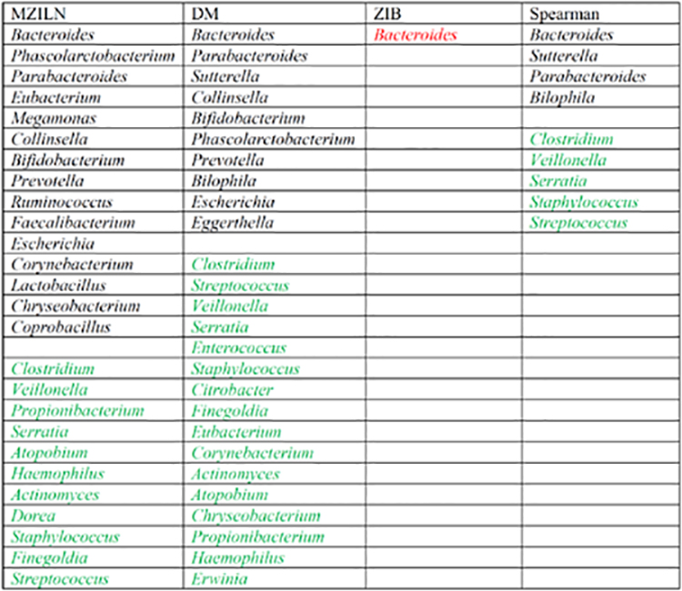
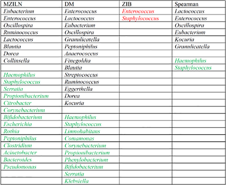
There were 28 genera selected for the association with delivery mode (Table 2), of which 17 genera had positive associations and 11 genera had negative associations. Compared with Madan and Hoen et al. [45] that only found 5 genera in association with delivery mode, although we missed two of their genera (Pectobacterium and Rothia), our approach found 23 more genera including Bifidobacterium, Clostridium and Streptococcus which are known to have important impact on children’s health [48–57]. There were 23 genera selected for association with feeding type (Table 3), of which 9 genera had positive associations and 14 genera had negative associations. Madan and Hoen et al. [45] found feeding type associated with only one genus (Lactococcus) which was also selected by our method, and in addition, we identified 2 2 more genera including Bacteroides, Bifidobacterium, Blautia and Enterococcus that have been linked to infant’s health in the literature [48, 57–64].

Table 2.

Genera identified to be associated with delivery mode. Black and green indicate positive and negative associations respectively. Red indicates that the direction of the identified association is unknown. The genera are sorted by association strength (measured by magnitude of estimated effect size or p value) from strongest to weakest in each category.

Table 3.

Genera identified to be associated with feeding type. Black and green indicate positive and negative associations respectively. Red indicates that the direction of the identified association is unknown. The genera are sorted by associatio n strength (measured by magnitude of estimated effect size or p value) from strongest to weakest in each category.

As a sensitivity analysis, we randomly chosen a different reference genus (Anoxybacillus) and reran our approach on the real data set, the selected genera are generally consistent (See Table 1A in the Appendix) especially for those with stronger associations. For example, the top 8 genera positively associated with feeding type are the same. The top 8 genera negatively associated with feeding type are also the same. For the genera positively associated with delivery mode, almost all genera are the same except 1 (out of 16) genus identified by reference genus Akkermansia was not identified by reference genus Anoxybacillus and 3 (out of 18) genera identified by reference genus Anoxybacillus were not identified by reference genus Akkermansia. For genera negatively associated with delivery mode, the top 4 genera identified by reference genus Anoxybacillus are among the top 6 genera identified by reference genus Akkermansia.

As a comparison, we also analyzed the data using DM, ZIB and SP. We also applied Wilcoxon rank sum test which generated nearly identical results as the SP approach, thus Wilcoxon test results were not presented. We did not include KPR in this comparison because KPR is not developed for testing the associations of binary variables with microbiome. FDR was set at 0.05 for ZIN and SP. Consistent with the simulation results, ZIB and SP found less genera than MZILN as shown in Tables 2 and 3. DM selected more taxa than expected and had good overlap with MZILN.

5. Discussion

This paper proposed an innovative MZILN model for analyzing microbiome RA in relation to health risk factors. The approach is based on a two-part model with the discrete part to handle excessive number of zeros commonly seen in microbiome sequencing data and the logistic-normal part to address the compositional structure of microbiome RA data. Standard regularization procedures such as LASSO, SCAD and MCP can be easily incorporated into this approach to obtain sparse estimations of high-dimensional regression parameters to avoid overfitting of the model. By borrowing the strength of estimating equations, the proposed approach can accommodate complex inter-taxa correlation structure induced by the phylogenetic hierarchical structure and the compositional data structure. Our simulation study has demonstrated the performance of our approach in comparison with existing methods. Our approach can be applied to RA of OTU, amplicon sequence variant and other RA data as well although the description in this paper has been focusing on analyzing taxa RA. R program is available upon request to implement the method. We are also working on building an R package.

Excessive zero data points could be due to biological reason or data collection technical reason. We assume a probability is associated with each data point (or combination of data points) being zero. All these probabilities can depend on the covariates through another set of regression equations. But because the probabilities are not our focus in this manuscript, we can treat them as nuisance parameters when the target of inference is the impact of the covariates on the non-zero part of the taxa (See details in Section S1 of the supplemental material). In essence, it is equivalent to a conditional regression where it is conditional on the taxa RA being non-zero. This kind of inference has been studied in the literature [24, 28] where FDR approach was used to deal with multiple testing whereas we employed regularization approaches to obviate concerns of multiple testing. Although we focus on the inference for the non-zero taxa, it is necessary to include the zero part in the model to formally describe the distribution of the data. In the future, we will develop methods that can handle high-dimensional parameters from both the non-zero part and zero part of microbial data.

Compared with the miLineage approach [24], an immediate advantage of our method is the flexibility to handle high-dimensional microbial taxa data (ie, number of taxa bigger than sample size) with regularization approaches whereas their approach has to analyze lineages to have a solution in such cases. Depending on what is needed in practice, our model can produce sparse estimates with individual ${\mathcal{l}}_1$ penalties as well as group ${\mathcal{l}}_1$ penalties. Our handling of high dimensionality is different than those methods that treat microbiome data as covariates instead of outcome variables [21, 23] where standard regularization approaches cannot be directly applied due to the compositional structure of the covariates. Penalized likelihood estimation methods have also been developed to analyze high-dimensional microbiome absolute abundance count data in relation to other covariates such as micronutrients [25, 26], but they are not as flexible as our method in terms of employing the penalization terms. Our estimator has a very simple form: ordinary least square (OLS) estimator, and thus naturally allows for all standard regularization approaches that can be applied for OLS estimators. A downside of our proposed approach is that we did not consider the zero-part in the estimation by treating the zero-part parameters as nuisance parameters. This may cause efficiency loss in the estimation process when microbiome data is extremely sparse. However, even with sparse data, the overall performance of our approach still is still better than other approaches according to the comparison in the simulation.

Compared with many existing methods developed to analyze RA data, one of the nice properties of our method is that we do not impute zero sequencing counts with a pseudo count (eg,0.5) or impute zero proportion with an arbitrary small proportion. When dealing with RA data, log-ratio transformation is often used to address the compositional data structure. However, log-ratio transformation can only be applied to non-zero RA, and thus imputation for zero RA is a commonly used technique in the literature which could distort the data and consequently distort the estimated associations. Our method does not need to impute zero RA’s by constructing the MZILN distribution that can appropriately handle the zero-inflated data structure.

Our approach allows for a very flexible inter-taxa correlation structure. There are two main drivers for the inter-taxa correlation: the inherent compositional data structure and the hierarchical phylogenetic tree structure. Compositional data structure induces negative correlations between taxa because all taxa RA sum to 1 and thus one RA increase is accompanied by the decrease of another RA. The phylogenetic tree structure reflects evolutionary relationships among microbes based upon similarities and differences in their genetic characteristics. It does not necessarily induce negative inter-taxa correlations. Depending on the functional relationships ef microbes, this hierarchical tree structure could generate positive or negative inter-taxa correlations. The compositional data structure and the hierarchical phylogenetic tree structure are compounded in the data and can generate complicated inter-taxa correlations. Our MZILN method adequately handle the complex correlation structure by utilizing powerful estimation tools from estimating equations approaches.

Although normal distribution is assumed for the leg-ratio transformation of the data, this assumption can be largely relaxed in practice since estimating equation (3) does net rely on the normal distribution assumption as long as the mean of the left side of equation (3) is 0. The robustness to mis-specification of distribution was demonstrated with a simulation. This allows real data analysis to address a much broader range of distributions, and thus it make the model a very useful tool for researchers to study associations of microbiome with ether variables of interest.

The proposed approach needs to select a reference taxon because of the definition of the logistic-normal distribution. Simulation study showed that results are reasonably stable across randomly selected reference taxa. In the real data application, we also saw good consistent results across two randomly selected reference taxa although there are some differences. Our method is flexible in choosing a reference taxon because it does not require the reference taxon to have non-zero RA for all samples. Nonetheless, it warrants further investigation to find the optimal reference taxon for the analysis which will be one of our future research topics.

Appendix

Comparison of selected genera under two randomly selected reference genera: Akkermansia and Anoxybacillus. Results for Akkermansia being the reference genus is also presented in Section 4.

Table 1A.

Genera associated with delivery mode and feeding type under two different reference genera. Black and green indicate positive and negative associations respectively. Genera are sorted by association strength (measured by magnitude of estimated effect size) from strongest to weakest in each category.

Genera associated with delivery mode		Genera associated with feeding type
Reference genus: Akkermansia	Reference genus: Anoxybadllus	Reference genus: Akkermansia	Reference genus: Anoxybadllus
Bacteroides	Bacteroides	Eubacterium	Eubacterium
Phascolarctobacterium	Parabacteroides	Enterococcus	Enterococcus
Parabacteroides	Phascolarctobacterium	Oscillospira	Oscillospira
Eubacterium	Eubacterium	Ruminococcus	Lactococcus
Megamonas	Collinsella	Lactococcus	Ruminococcus
Collinsella	Bifidobacterium	Blautia	Blautia
Bifidobacterium	Sutterella	Dorea	Dorea
Prevotella	Prevotella	Collinsella	Collinsella
Ruminococcus	Limnohabitans		Eggerthella
Faecalibacterium	Ruminococcus	Haemophilus	Parabacteroides
Escherichia	Megamonas	Staphylococcus	Granulicatella
Corynebacterium	Escherichia	Serratia	Veillonella
Lactobacillus	Faecalibacterium	Propioni bacterium	Streptococcus
Chryseobacterium	Lactobacillus	Citrobacter	Lactobacillus
Coprobacillus	Corynebacterium	Coryne bacterium
	Acinetobacter	Bifidobacterium	Staphylococcus
Clostridium	Chryseobacterium	Escherichia	Haemophilus
Veillonella		Rothia	Serratia
Propionibacterium	Clostridium	Peptoniphilus	Propionibacteriu
Serratia	Veillonella	Clostridium	Bifidobacterium
Amiddleobium	Serratia	Acinetobacter	Citrobacter
Haemophilus	Haemophilus	Bacteroides	Corynebacterium
Actinomyces	Staphylococcus	Pseudomonas	Pseudomonas
Dorea	Actinomyces		Rothia
Staphylococcus			Escherichia
Finegoldia			Acinetobacter
Streptococcus

References

- 1.Blaser MJ. The microbiome revolution. J Clin Invest 2014; 124: 4162–4165. [DOI] [PMC free article] [PubMed] [Google Scholar]
- 2.Cho I, Blaser MJ. The human microbiome: at the interface of health and disease. Nat Rev Genet 2012; 13: 260–270. [DOI] [PMC free article] [PubMed] [Google Scholar]
- 3.Turnbaugh PJ, Ley RE, Hamady M, Fraser-Liggett CM, Knight R, Gordon JI. The human microbiome project. Nature 2007; 449: 804–810. [DOI] [PMC free article] [PubMed] [Google Scholar]
- 4.Chen Y, Blaser MJ. Inverse associations of Helicobacter pylori with asthma and allergy. Arch Intern Med 2007; 167: 821–827. [DOI] [PubMed] [Google Scholar]
- 5.Hoen AG, Li J, Moulton LA, O’Toole GA, Housman ML, Koestler DC, Guill MF, Moore JH, Hibberd PL, Morrison HG, Sogin ML, Karagas MR, Madan JC. Associations between Gut Microbial Colonization in Early Life and Respiratory Outcomes in Cystic Fibrosis. Journal of Pediatrics 2015; 167: 138–U520. [DOI] [PMC free article] [PubMed] [Google Scholar]
- 6.Madan JC, Salari RC, Saxena D, Davidson L, O’Toole GA, Moore JH, Sogin ML, Foster JA, Edwards WH, Palumbo P, Hibberd PL. Gut microbial colonisation in premature neonates predicts neonatal sepsis. Arch Dis Child Fetal Neonatal Ed 2012; 97: F456–462. [DOI] [PMC free article] [PubMed] [Google Scholar]
- 7.Castellarin M, Warren RL, Freeman JD, Dreolini L, Krzywinski M, Strauss J, Barnes R, Watson P, Allen-Vercoe E, Moore RA, Holt RA. Fusobacterium nucleatum infection is prevalent in human colorectal carcinoma. Genome Research 2012; 22: 299–306. [DOI] [PMC free article] [PubMed] [Google Scholar]
- 8.McColl KE. Clinical practice. Helicobacter pylori infection. N Engl J Med 2010; 362: 1597–1604. [DOI] [PubMed] [Google Scholar]
- 9.Reikvam DH, Erofeev A, Sandvik A, Grcic V, Jahnsen FL, Gaustad P, McCoy KD, Macpherson AJ, Meza-Zepeda LA, Johansen FE. Depletion of murine intestinal microbiota: effects on gut mucosa and epithelial gene expression. Plos One 2011; 6: e17996. [DOI] [PMC free article] [PubMed] [Google Scholar]
- 10.Trasande L, Blustein J, Liu M, Corwin E, Cox LM, Blaser MJ. Infant antibiotic exposures and early-life body mass. Int J Obes (Lond) 2013; 37: 16–23. [DOI] [PMC free article] [PubMed] [Google Scholar]
- 11.Turnbaugh PJ, Ley RE, Mahowald MA, Magrini V, Mardis ER, Gordon JI. An obesity-associated gut microbiome with increased capacity for energy harvest. Nature 2006; 444: 1027–1031. [DOI] [PubMed] [Google Scholar]
- 12.Thomas T, Gilbert J, Meyer F. Metagenomics - a guide from sampling to data analysis. Microb Inform Exp 2012; 2: 3. [DOI] [PMC free article] [PubMed] [Google Scholar]
- 13.Tringe SG, Rubin EM. Metagenomics: DNA sequencing of environmental samples. Nat Rev Genet 2005; 6: 805–814. [DOI] [PubMed] [Google Scholar]
- 14.Cole JR, Wang Q, Cardenas E, Fish J, Chai B, Farris RJ, Kulam-Syed-Mohideen AS, McGarrell DM, Marsh T, Garrity GM, Tiedje JM. The Ribosomal Database Project: improved alignments and new tools for rRNA analysis. Nucleic Acids Research 2009; 37: D141–145. [DOI] [PMC free article] [PubMed] [Google Scholar]
- 15.Segata N, Waldron L, Ballarini A, Narasimhan V, Jousson O, Huttenhower C. Metagenomic microbial community profiling using unique clade-specific marker genes. Nature Methods 2012; 9: 811–+. [DOI] [PMC free article] [PubMed] [Google Scholar]
- 16.Li HZ. Microbiome, Metagenomics, and High-Dimensional Compositional Data Analysis. Annual Review of Statistics and Its Application, Vol 2 2015; 2: 73–94. [Google Scholar]
- 17.Chen J, Bittinger K, Charlson ES, Hoffmann C, Lewis J, Wu GD, Collman RG, Bushman FD, Li HZ. Associating microbiome composition with environmental covariates using generalized UniFrac distances. Bioinformatics 2012; 28: 2106–2113. [DOI] [PMC free article] [PubMed] [Google Scholar]
- 18.Mccoy CO, Matsen FA. Abundance-weighted phylogenetic diversity measures distinguish microbial community states and are robust to sampling depth. Peerj 2013; 1. [DOI] [PMC free article] [PubMed] [Google Scholar]
- 19.La Rosa PS, Brooks JP, Deych E, Boone EL, Edwards DJ, Wang Q, Sodergren E, Weinstock G, Shannon WD. Hypothesis Testing and Power Calculations for Taxonomic-Based Human Microbiome Data. Plos One 2012; 7. [DOI] [PMC free article] [PubMed] [Google Scholar]
- 20.McMurdie PJ, Holmes S. Waste Not, Want Not: Why Rarefying Microbiome Data Is Inadmissible. Plos Computational Biology 2014; 10. [DOI] [PMC free article] [PubMed] [Google Scholar]
- 21.Lin W, Shi PX, Feng R, Li HZ. Variable selection in regression with compositional covariates. Biometrika 2014; 101: 785–797. [Google Scholar]
- 22.Randolph T, Zhao S, Copeland W, Hullar M, Shojaie A. Kernel-Penalized Regression for Analysis of Microbiome Data. Annals of Applied Statistics In press. [DOI] [PMC free article] [PubMed] [Google Scholar]
- 23.Shi P, Zhang A, Li HZ. Regression Analysis for Microbiome Compositional Data. Annals of Applied Statistics 2016; In press. [Google Scholar]
- 24.Tang ZZ, Chen GH, Li HZ. A General Framework for Association Analysis of Microbial Community on a Taxonomic Tree. Bioinformatics 2017; 33: 1278–1285. [DOI] [PMC free article] [PubMed] [Google Scholar]
- 25.Chen J, Li HZ. Variable Selection for Sparse Dirichlet-Multinomial Regression with an Application to Microbiome Data Analysis. Annals of Applied Statistics 2013; 7: 418–442. [DOI] [PMC free article] [PubMed] [Google Scholar]
- 26.Xia F, Chen J, Fung WK, Li HZ. A Logistic Normal Multinomial Regression Model for Microbiome Compositional Data Analysis. Biometrics 2013; 69: 1053–1063. [DOI] [PubMed] [Google Scholar]
- 27.Peng X, Li G, Liu Z. Zero-Inflated Beta Regression for Differential Abundance Analysis with Metagenomics Data. J Comput Biol 2015. [DOI] [PMC free article] [PubMed] [Google Scholar]
- 28.Chen EZ, Li HZ. A two-part mixed-effect model for analyzing longitudinal microbiome compositional data. Bioinformatics 2016; In press. [DOI] [PMC free article] [PubMed] [Google Scholar]
- 29.Liang KY, Zeger SL. Longitudinal Data-Analysis Using Generalized Linear-Models. Biometrika 1986; 73: 13–22. [Google Scholar]
- 30.Tibshirani R Regression shrinkage and selection via the Lasso. Journal of the Royal Statistical Society Series B-Methodological 1996; 58: 267–288. [Google Scholar]
- 31.Fan J, Li R. Variable selection via nonconvace penalized likelihood and its oracle properties. Journal of American Statistical Association 2001; 96: 1348–1360. [Google Scholar]
- 32.Zhang CH. Nearly Unbiased Variable Selection under Minimax Concave Penalty. Annals of Statistics 2010; 38: 894–942. [Google Scholar]
- 33.Farzan SF, Korrick S, Li Z, Enelow R, Gandolfi AJ, Madan J, Nadeau K, Karagas MR. In utero arsenic exposure and infant infection in a United States cohort: a prospective study. Environmental Research 2013; 126: 24–30. [DOI] [PMC free article] [PubMed] [Google Scholar]
- 34.Aitchison J The statistical analysis of compositional data. Blackburn Press: Caldwell, N.J., 2003. [Google Scholar]
- 35.Aitchison J The Statistical-Analysis of Compositional Data. Journal of the Royal Statistical Society Series B-Methodological 1982; 44: 139–177. [Google Scholar]
- 36.Teugels JL. Some Representations of the Multivariate Bernoulli and Binomial Distributions. Journal of Multivariate Analysis 1990; 32: 256–268. [Google Scholar]
- 37.Dai B, Ding SL, Wahba G. Multivariate Bernoulli distribution. Bernoulli 2013; 19: 1465–1483. [Google Scholar]
- 38.Billheimer D, Guttorp P, Fagan WF. Statistical interpretation of species composition. Journal of the American Statistical Association 2001; 96: 1205–1214. [Google Scholar]
- 39.Yuan M, Lin Y. Model selection and estimation in the Gaussian graphical model. Biometrika 2007; 94: 19–35. [Google Scholar]
- 40.Godambe VP. Estimating functions: New York, 1991. [Google Scholar]
- 41.Zou H The Adaptive Lasso and Its Oracle Properties. Journal of the American Statistical Association 2006; 101: 1418–1429. [Google Scholar]
- 42.Zou H, Hastie T. Regularization and variable selection via the elastic net. Journal of the Royal Statistical Society: Series B 2005; 67: 301–320. [Google Scholar]
- 43.Zhao S, Shojaie A. A significance test for graph-constrained estimation. Biometrics 2016; 72: 484493. [DOI] [PMC free article] [PubMed] [Google Scholar]
- 44.Farzan SF, Korrick S, Li ZG, Enelow R, Gandolfi AJ, Madan J, Nadeau K, Karagas MR. In utero arsenic exposure and infant infection in a United States cohort: A prospective study. Environmental Research 2013; 126: 24–30. [DOI] [PMC free article] [PubMed] [Google Scholar]
- 45.Madan JC, Hoen AG, Lundgren SN, Farzan SF, Cottingham KL, Morrison HG, Sogin ML, Li H, Moore JH, Karagas MR. Association of Cesarean Delivery and Formula Supplementation With the Intestinal Microbiome of 6-Week-Old Infants. JAMA Pediatr 2016; 170: 212–219. [DOI] [PMC free article] [PubMed] [Google Scholar]
- 46.Degnan PH, Ochman H. Illumina-based analysis of microbial community diversity. ISME J 2012; 6: 183–194. [DOI] [PMC free article] [PubMed] [Google Scholar]
- 47.Caporaso JG, Lauber CL, Walters WA, Berg-Lyons D, Huntley J, Fierer N, Owens SM, Betley J, Fraser L, Bauer M, Gormley N, Gilbert JA, Smith G, Knight R. Ultra-high-throughput microbial community analysis on the Illumina HiSeq and MiSeq platforms. ISME J 2012; 6: 1621–1624. [DOI] [PMC free article] [PubMed] [Google Scholar]
- 48.Turroni F, Ribbera A, Foroni E, van Sinderen D, Ventura M. Human gut microbiota and bifidobacteria: from composition to functionality. Antonie Van Leeuwenhoek 2008; 94: 35–50. [DOI] [PubMed] [Google Scholar]
- 49.Parracho HM, Bingham MO, Gibson GR, McCartney AL. Differences between the gut microflora of children with autistic spectrum disorders and that of healthy children. J Med Microbiol 2005; 54: 987–991. [DOI] [PubMed] [Google Scholar]
- 50.Russell SL, Gold MJ, Hartmann M, Willing BP, Thorson L, Wlodarska M, Gill N, Blanchet MR, Mohn WW, McNagny KM, Finlay BB. Early life antibiotic-driven changes in microbiota enhance susceptibility to allergic asthma. EMBO Rep 2012; 13: 440–447. [DOI] [PMC free article] [PubMed] [Google Scholar]
- 51.Bisgaard H, Li N, Bonnelykke K, Chawes BL, Skov T, Paludan-Muller G, Stokholm J, Smith B, Krogfelt KA. Reduced diversity of the intestinal microbiota during infancy is associated with increased risk of allergic disease at school age. J Allergy Clin Immunol 2011; 128: 646–652 e641–645. [DOI] [PubMed] [Google Scholar]
- 52.Cong X, Xu W, Romisher R, Poveda S, Forte S, Starkweather A, Henderson WA. Gut Microbiome and Infant Health: Brain-Gut-Microbiota Axis and Host Genetic Factors. The Yale Journal of Biology and Medicine 2016; 89: 299–308. [PMC free article] [PubMed] [Google Scholar]
- 53.Kinross JM, Darzi AW, Nicholson JK. Gut microbiome-host interactions in health and disease. Genome Med 2011; 3: 14. [DOI] [PMC free article] [PubMed] [Google Scholar]
- 54.Mueller NT, Bakacs E, Combellick J, Grigoryan Z, Dominguez-Bello MG. The infant microbiome development: mom matters. Trends Mol Med 2015; 21: 109–117. [DOI] [PMC free article] [PubMed] [Google Scholar]
- 55.Munyaka PM, Khafipour E, Ghia JE. External influence of early childhood establishment of gut microbiota and subsequent health implications. Front Pediatr 2014; 2: 109. [DOI] [PMC free article] [PubMed] [Google Scholar]
- 56.Vangay P, Ward T, Gerber JS, Knights D. Antibiotics, pediatric dysbiosis, and disease. Cell Host Microbe 2015; 17: 553–564. [DOI] [PMC free article] [PubMed] [Google Scholar]
- 57.Sjogren YM, Tomicic S, Lundberg A, Bottcher MF, Bjorksten B, Sverremark-Ekstrom E, Jenmalm MC. Influence of early gut microbiota on the maturation of childhood mucosal and systemic immune responses. Clin Exp Allergy 2009; 39: 1842–1851. [DOI] [PubMed] [Google Scholar]
- 58.Rutayisire E, Huang K, Liu Y, Tao F. The mode of delivery affects the diversity and colonization pattern of the gut microbiota during the first year of infants’ life: a systematic review. BMC Gastroenterol 2016; 16: 86. [DOI] [PMC free article] [PubMed] [Google Scholar]
- 59.Penders J, Thijs C, Vink C, Stelma FF, Snijders B, Kummeling I, van den Brandt PA, Stobberingh EE. Factors influencing the composition of the intestinal microbiota in early infancy. Pediatrics 2006; 118: 511–521. [DOI] [PubMed] [Google Scholar]
- 60.Mazmanian SK, Round JL, Kasper DL. A microbial symbiosis factor prevents intestinal inflammatory disease. Nature 2008; 453: 620–625. [DOI] [PubMed] [Google Scholar]
- 61.Corvaglia L, Tonti G, Martini S, Aceti A, Mazzola G, Aloisio I, Di Gioia D, Faldella G. Influence of Intrapartum Antibiotic Prophylaxis for Group B Streptococcus on Gut Microbiota in the First Month of Life. J Pediatr Gastroenterol Nutr 2016; 62: 304–308. [DOI] [PubMed] [Google Scholar]
- 62.Bjorksten B, Sepp E, Julge K, Voor T, Mikelsaar M. Allergy development and the intestinal microflora during the first year of life. J Allergy Clin Immunol 2001; 108: 516–520. [DOI] [PubMed] [Google Scholar]
- 63.Azad MB, Konya T, Persaud RR, Guttman DS, Chari RS, Field CJ, Sears MR, Mandhane PJ, Turvey SE, Subbarao P, Becker AB, Scott JA, Kozyrskyj AL. Impact of maternal intrapartum antibiotics, method of birth and breastfeeding on gut microbiota during the first year of life: a prospective cohort study. Bjog 2016; 123: 983–993. [DOI] [PubMed] [Google Scholar]
- 64.Hoen AG, Li J, Moulton LA, O’Toole GA, Housman ML, Koestler DC, Guill MF, Moore JH, Hibberd PL, Morrison HG, Sogin ML, Karagas MR, Madan JC. Associations between Gut Microbial Colonization in Early Life and Respiratory Outcomes in Cystic Fibrosis. J Pediatr 2015; 167: 138–147. e131–133. [DOI] [PMC free article] [PubMed] [Google Scholar]
Associated Data
This section collects any data citations, data availability statements, or supplementary materials included in this article.