Distributed Learning from Multiple EHR Databases: Contextual Embedding Models for Medical Events

Abstract

Electronic health record (EHR) data provide promising opportunities to explore personalized treatment regimes and to make clinical predictions. Compared with regular clinical data, EHR data are known for their irregularity and complexity. In addition, analyzing EHR data involves privacy issues and sharing such data is often infeasible among multiple research sites due to regulatory and other hurdles. A recently published work uses contextual embedding models and successfully builds one predictive model for more than seventy common diagnoses. Despite of the high predictive power, the model cannot be generalized to other institutions without sharing data. In this work, a novel method is proposed to learn from multiple databases and build predictive models based on Distributed Noise Contrastive Estimation (Distributed NCE). We use differential privacy to safeguard the intermediary information sharing. The numerical study with a real dataset demonstrates that the proposed method not only can build predictive models in a distributed manner with privacy protection, but also preserve model structure well and achieve comparable prediction accuracy. The proposed methods have been implemented as a stand-alone Python library and the implementation is available on Github (https://github.com/ziyili20/DistributedLearningPredictor) with installation instructions and use-cases.

Introduction

As promoted by the 2009 Health Information Technology for Economic and Clinical Health (HITECH) Act, more than ninety percent of the office-based physician practices adopted Electronic Health Records (EHR) systems to store patient clinical documents at the end of 2017¹. As a substitution of paper-based records, EHR systems usually include information from multiple clinical aspects, such as symptoms, laboratory test results, prescriptions, diagnoses, and doctor notes. This information not only contains the health history and disease progression of each patient, but also reflects how diseases are treated in general. Thus EHR data is a rich depository for understanding disease features and treatment regimes.

Although EHR data are informative, analyzing EHR data can be a challenging task. As described in Hripcsak² and Cheng³, EHR data are usually complex, inaccurate, irregular, sparse and of high-dimensionality. The large volume of EHR data can make storage non-trivial, and analyzing such data involves a lot of challenges. Besides its complexity, obtaining access or sharing EHR data can also be complicated, since the use of EHR data involves high-level privacy-preserving requirements⁴.

There has been a growing body of research on the analysis of EHR data. Existing work mainly utilizes information from EHR data for two goals: medical event phenotyping and predictive model construction. For the task of extracting features from EHR data (i.e. medical event phenotying), Batal⁵ uses temporal pattern mining to obtain abstraction sequences, which can be further applied in predictive models. Liu⁶ uses temporal graphs to construct graph-based frameworks from EHR data and to understand phenotype relationships. A recent work by Beaulieu-Jones⁷ maps patient trajectories through longitudinal extraction and deep learning models, which also provides meaningful embeddings for medical events. At the same time, the direction of obtaining low dimensional vector representation for medical events using deep-learning methods has advanced quickly. Several works have published applications on this topic^8-12, showing dense and low-dimensional representation provides meaningful interpretation in terms of events similarity. Additional benefit is that low dimensional representations are easy to be applied in downstream analyses, such as identifying disease susceptible populations or disease subtypes as well as making predictions for diagnoses or clinical outcomes.

Among various tasks, prediction model construction is among the most important ones. Many attempts have been made recently and been shown promising^{3, 13-16}. Although many predictive methods have been proposed, limitations and gaps still exist in real world applications. For one thing, most of the models proposed target only one or two diseases. In real life, at least a number of common diseases should be considered for prediction. And for another, almost all the current methods assume that training data come from one source or training data come from multiple datasets but are available from one single place. A real scenario might be that more than one database is available at different sites but cannot be transferred or shared. It would be preferable if a model can learn from multiple EHR datasets and at the same time predict the occurrence of multiple diseases.

In this article, we propose the Distributed Noise Contrastive Estimation (Distributed NCE), a neural-network-based technique for building predictive models of patient diagnoses. This method can learn from multiple EHR databases without sharing data among sites and make predictions for more than seventy common diseases. Our work is an extension of the Word2Vec model by Mikolov¹⁷ and the Patient-Diagnosis Projection Similarity Model by Farhan¹⁸. The main contribution of our work is to incorporate information from multiple data sources in one global model while preserving the privacy of underlying private data. As many methods have been developed based on Word2Vec^19-21, the proposed approach is notable in that it can be generalized to any Word2Vec-based model or other neural network based model to expand data sources while protecting patient privacy.

Two recent works has been published and are focusing on similar problem^{22, 23}. Huang et al. uses a privacy-preserving harmonization approach based on an existing method called “Procrustes” to map the vectors learned from Word2Vec in one site to the vectors of another site²². Lee et al. does not use Word2Vec but develops a hashing technique to lower the dimension of patient features. They utilize a multi-hashing technique and demonstrate better results than existing uni-hashing methods²³. Different from Lee et al., we propose to utilize Word2Vec to obtain lower-dimension representations of patient features, and different from Huang et al., our method directly modify the algorithm of Word2Vec to make it incorporate the information from two hospitals.

The remainder of this article is structured as follows. The preliminary works are presented in section 2, problem setting and the proposed method Distributed NCE in section 3, two alternative methods including Naive Updates and Dropout Updates in section 4, the numerical study using real data in section 5, and some comments and discussions in section 6.

1. Preliminaries

This section reviews two existing models, which form the foundation of the proposed methods. We first briefly discuss the skip-gram (SG) model, a popular model used in the Word2Vec algorithm. This model has a three-layer neural network and uses each single word to predict the context words surrounding it. Then we review the Patient-Diagnosis Projection Similarity (PDPS) model based on the SG model.

1.1. Skip-gram Model

Following the text-inspired notation in Mikolov²⁴, suppose there is a training sequence consisted of words ω₁, ω₂,…, ω_T. A three-layer neural network is constructed as demonstrated in Figure 1. The input layer is a vector representing a single word in the training sequence and the output layer is vectors representing the context words around the input word. The hidden layer has the same number of nodes as the dimension of vector representation, as the weights from input layer to hidden layer are used as lower-dimensional representations. The dimension of vector representation is a tuning parameter that the users can change, and we fix it as 350 in all the experiments. The weight matrix from input layer to hidden layer is denoted by W and the weight matrix from hidden layer to output layer by W*. The goal is to maximize the log-likelihood of context words given an input word:

$$\frac{1}{T}\sum _{t=1}^{T}log\mathcal{P}({\omega }_{t-c},\dots ,{\omega }_{t-1},{\omega }_{t+1},\dots ,{\omega }_{t+c}\mid {\omega }_t)=\frac{1}{T}\sum _{t=1}^T\underset{j\ne 0}{\sum _{-c\le j\le c}}log\mathcal{P}({\omega }_{t+j}\mid {\omega }_t)$$ (1)

ω_t is the input word and ω_t−c,…, ω_t−1, ω_t+1,…, ω_t+c are the context words around ω_t. The conditional probability of observing an output word (or an aforementioned context word) ω₀ ∈ {ω_t−c,…, ω_t−1, ω_t+1,…, ω_t+c} given the input word ω_I is defined as:

$$\mathcal{P}({\omega }_O\mid {\omega }_I)=\frac{exp(v_{{\omega }_O}^{\ast }{}^T{v}_{{\omega }_I})}{{\sum }_{\omega =1}^{n_w}exp(v_{\omega }^{\ast }{}^T{v}_{{\omega }_I})}$$ (2)

Figure 1.

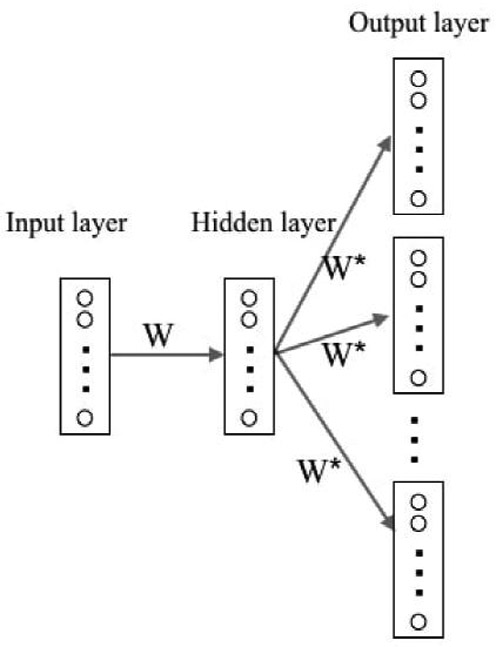
Demonstration of SG model structures. One square is a vector representation of one word. Circles represent elements in each vector. W is the weight between input layer and hidden layer, W* is the weight between hidden layer and output layer.

Here n_w is the number of words in the vocabulary, v_ωI is the corresponding weight vector for word ω_I in matrix W, and $v_{{\omega }_O}^{\ast }$ is the corresponding weight vector for word ω_O in matrix W*. Note that if ω_I is the i—th word in vocabulary and ω_O is the j—th word, v_ωI and $v_{{\omega }_O}^{\ast }$ are the i—th column of W and the j—th column of W* respectively representing the input and output vector of ω_I and ω_O. Thus the SG model adjusts two neural network weight matrices W and W* by maximizing the sum of log-likelihood for pairs consisted of all input words and their context words.

1.2. Patient-Diagnosis Projection Similarity Model

Farhan¹⁸ proposed a Word2Vec-based model, known as the patient-diagnosis projection similarity (PDPS), to predict patient diagnoses based on EHR data. Assume one has obtained a vector for all events by building an SG model on training datasets. Given a new patient sequence S which consists of his/her medical event codes ordered by time, the goal is to seek the optimal predicted diagnosis d* using S and the vector representations for all known medical events belonging to this subject.

Specifically, let $\mathcal{E}$ be the set of all possible events and $\mathcal{D}$ be the set of all possible diagnoses, and then stipulate that $\mathcal{D}$ is a subset of $\mathcal{E}$. For an event $e\in \mathcal{E}$, denote the vector representation of e by V_e. We represent a diagnosis element of $\mathcal{D}$ by d and denote the vector representation for d by V_d. In order to incorporate the time effect of each medical event in sequence S, we calculate the time elapsed between the event e and the last event denoted by t_e.

To find the optimal prediction of diagnosis for a patient with EHR sequence S, PDPS finds

$$d^{\ast }=\text{arg}\underset{d\in \mathcal{D}}{\text{max}}CS(V_d,\frac{{\sum }_{e\in s}{V}_{e}exp(-\lambda t_e)}{{\sum }_{e\in S}exp(-\lambda t_e)})$$ (3)

where CS(x, y) is the cosine similarity between x and y, λ is the decay factor and usually takes a value between 0 and 1, $\mathcal{D}$ is the list of all diagnoses in the vocabulary. PDPS makes prediction based on the tendency (a scaler between 0 and 1 with higher value indicates more tendency) for a specified diagnosis $\tilde{d}$ with $CS(V_{\tilde{d}},\frac{{\sum }_{e\in S}{V}_e\mathit{exp}(-\lambda t_e)}{{\sum }_{e\in S}\mathit{exp}(-\lambda t_e)})$ so that the importance of distant medical events decay over time (following an exponential distribution). PDPS has previously demonstrated reasonable prediction performance (over more than 70 common diagnoses). But it was done in a centralized setting without considering the collaborative needs of privacy-preserving data sharing, which is common due to policy and regulation.

2. Distributed Noise Contrastive Estimation

To build a global model from multiple databases without sharing data, a novel technique is proposed and called Distributed Noise Contrastive Estimation (Distributed NCE). This section first presents the problem of interest. Then the proposed method Distributed NCE is elaborated. To allay the potential privacy concern when using Distributed NCE, Distributed NCE is further extended by adding differential privacy.

2.1. Problem Setting

Without loss of generality, we consider the case with two EHR databases D₁ and D₂, where the goal is to construct a predictive model on these two datasets with the constraint that D₁ and D₂ cannot be shared between sites and have to be analyzed locally. As mentioned above, this scenario happens when hospitals are not willing to share their EHR data due to policy or other concerns but would like to collaborate. In this case, methods of constructing a predictive model distributedly are desired. In the following section, we propose a novel technique, Distributed NCE, which can incorporate multiple datasets distributedly. The proposed method can be applied on PDPS or other Word2Vec-based predictive models.

When D₁ and D₂ have the same vocabulary of medical events or D₂ includes only a subset of D₁’s vocabulary, the model built by D₁ can be updated easily using D₂ in the Word2Vec model. But D₁ and D₂ do not always have the same vocabularies. Different institutions might observe different medical events or measure different labs. Such inconsistency leads to the discrepancies in vocabulary.

2.2. Distributed Noise Contrastive Estimation (NCE)

Our idea of the Distributed NCE is inspired by the main hurdle of learning from multiple databases - discrepancies between vocabularies. Our proposed solution is to obtain vocabularies from multiple sites first and initialize an empty neural network model. Then this model can be trained using separate data sites in a sequential order. It is worth noting that, the iterations of Word2Vec are performed within each site at training stage and no inter-site iterations are required in the training phase. After all the data sites have trained the model, a global model is built and the weights between input and hidden layers are the final vector for medical events. This method is effective because it exactly mimics the process of training a Word2Vec model. The original training process feeds batches of the document corpus into the gradient-descent algorithms, which is what Distributed NCE would do except that Distributed NCE operates on a corpus in two separate locations. The Distributed NCE method is demonstrated in Figure 2.

Figure 2.

Distributed NCE. Squares represent medical events. Crosses represent counts of medical events. After obtaining the vocabularies from datasets D₁ and D₂, the event lists and event counts are merged. Neural network is trained sequentially using D₁ and D₂.

Suppose one has access to two databases D₁ and D₂, the vocabulary of database D₁ has size n_w and the vocabulary of database D₂ has $n_w^{\ast }$ new words. In the SG model, objective function (1) is unchanged but the conditional probability of observing an input work is changed from function (2) to (4). The only difference in equation (2) and (4) is that in the proposed model, the training procedures take place with an expanded vocabulary $n_w+n_w^{\ast }$ in all data sites even if some of the medical events in this vocabulary is present only in a subset of data sites.

$$\mathcal{P}({\omega }_O\mid {\omega }_I)=\frac{exp(v_{{\omega }_O}^{\ast }{}^T{v}_{{\omega }_I})}{{\sum }_{\omega =1}^{n_w+n_w^{\ast }}exp(v_{\omega }^{\ast }{}^T{v}_{{\omega }_I})}$$ (4)

One challenge of the calculation using equation (4) is that the denominator part iterates over all words in the expanded vocabulary, which can be computationally intensive. To tackle this challenge, we use NCE as an optimization technique to approximates the empirical distribution of “context” in equation (4) to avoid the step of iterating over all vocabularies²⁵. In NCE, the global counts are used to obtain the “flattened” empirical unigram distribution (by exponentiating each probability by 0 < α < 1 and re-normalizing)²⁶. In this way, we maintain a faithful language model in a global sense as opposed to the other sampling strategy (such as negative sampling), which fails to approximate the empirical distribution with their respective model distribution. There is an existing package called “Online Word2Vec”²⁷ which has similar spirit. But Distributed NCE uses global vocabulary and count table in optimizations, resulting in closer results to a global model.

To illustrate how NCE works, we symbolically represent the weight matrices W and W* by θ = (W, W*). We denote $u_{\theta }({\omega }_O,{\omega }_I)=\mathit{exp}({v_{{\omega }_O}^{\ast }}^T{v}_{{\omega }_I})$ to be the function that assign a score to the word ω_O in context ω_I. To facilitate the estimation, a “noise” distribution is assumed, and denoted by q(ω). NCE finds the optimal solution for θ which maximizes the objective function,

$${\theta }^{\ast }=\underset{\theta }{\text{argmax}}\sum _{({\omega }_O,{\omega }_I)\in V}\left(\log \frac{u_{\theta }({\omega }_O,{\omega }_I)}{u_{\theta }({\omega }_O,{\omega }_I)+kq(\omega )}+\sum _{i=1,\stackrel{‒}{\omega }\sim q(\omega )}^k\log \frac{kq(\stackrel{‒}{\omega })}{u_{\theta }(\stackrel{‒}{\omega },{\omega }_I)+kq(\stackrel{‒}{\omega })}\right)$$ (5)

In optimizing equation 5, k negative samples are drawn from noise distribution q(ω) in each iteration and the global count table is used to estimate such q(ω). In another word, NCE uses an approximated objective function (5) to replace the previously computationally expensive function (4), and at the same time maintain the model structure close to the original model.

With N distinct datasets D₁, D₂, ⋯, D_N, Distributed NCE can be similarly applied using the procedures described in Figure 2. The first step is to collect and merge vocabularies of all these databases and build an empty Word2Vec model. Then one can consecutively train the model using databases from D₁ to D_N.

In implementation, we notice that Distributed NCE may have privacy concerns in the step of obtaining vocabulary counts if only two datasets are involved. The fact that one site can infer the medical event word counts of the other site from the global model may leak private information of patients, especially those with rare diseases. To address such concerns, the following section discusses how to add privacy protection in combined vocabulary and word counts.

2.3. Distributed Noise Contrastive Estimation with Privacy Protection

To protect data privacy when two datasets are analyzed by the Distributed NCE, a differential privacy (DP) component²⁸ is added into Distributed NCE. We call this method Distributed NCE with DP. The DP procedures are conducted at each data site independently. Only the DP-added count table are shared across sites to present the leakage of sensitive patient event information.

The DP method is proposed by Xiao²⁸ and its full name is differentially private histogram release through multidimensional partitioning. Given a vocabulary and the count table of all the words in vocabulary, in order to implement DP, the first step is to partition the count table into a few clusters. We use common methods such as k-means clustering or hierarchical clustering to partition the count list. In the next step, every value in one partition is replaced by the mean value plus random Laplace noise. The general workflow of adding DP to a one-dimensional data is illustrated in Figure 3. It is worth noting that we use global count to generate DP table, which is the only information shared and it helps harmonize the model.

Figure 3.

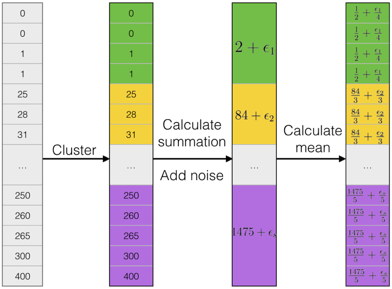
A symbolic illustration of implementing differential privacy on one-dimensional data. To apply DP on one-dimensional vectors, partition counts to subgroups in the first step. For each subgroup, calculate summations and add noise to group summations. Last, average summations to individual cells.

Suppose the whole count table x₁,…, x_N is divided into s partitions using some clustering technique. N is the number of words in vocabulary. The i—th partition contains elements x_i,1,…, x_i,N_i, i = 1,…, s. N_i is the number of elements in the i—th partition. To use the DP on the i—partition, each element is replaced by

$${\widehat{x}}_{i,j}=\frac{x_{i,1}+\cdots +x_{i,N_i}}{N_i}+\frac{{\epsilon }_i}{N_i},i=1,\dots ,s;j=1,\dots ,N_i.$$ (6)

Laplace noise ε_i is generated from $\mathit{Lap}(\frac{S_Q}{\alpha })$. Here we follow the notations used in Xiao²⁸. S_Q is the sensitivity of a query and α is a parameter controlling the strength of privacy protection. α usually takes a value smaller than 1 and the smaller α leads to stronger protection.

In the following applications, we adopt k-means clustering as the partition method and use different k values ranging from 10 to 150. The sensitivity of this problem is 2 since any change from one word to another in the histogram can only lead to change of the L — 1 distance of two vectors by 2, which makes S_Q equal 2. And we choose 0.001 as the value for α. Generally speaking, more partitions introduce more noise into the model, since creating s partitions means adding noise s times. But at the same time adding DP with more partitions results in tighter sub-groups and the group mean values closer to the original Distributed NCE without DP. Thus choosing the number of partitions is a trade-off between value accuracy and noise.

3. Two alternative solutions

This section describes two additional methods as alternatives to Distributed NCE. They are compared with Distributed NCE in our experiments. The first one, called “naive updates”, directly expands vocabulary when updating an existing Word2Vec model with a new dataset. The second method, called “dropout updates”, is inspired by the dropout technique commonly used in neural networks to avoid overfitting.

3.1. Naive updates

Suppose a Word2Vec model M₁ trained by the first dataset D₁ (see Section 1.1) has already been obtained, it can be updated by expanding the vocabulary of M₁ and adding input nodes and output nodes to the existing neural network. In the expanded model, denoted by M₂, the weights inherited from M₁ are initialized by the existing values in M₁ and new weights are randomly initialized. Then we train M₂ with new data D₂.

Assume the input layer, hidden layer, and output layer of M₁ have nodes {x₁,x₂,…,x_N1}, {h₁, h₂,…, h_L}, and {y₁,y₂,…,y_N1} respectively. N₁ is the number of words in vocabulary of D₁ and L is the number of nodes in hidden layer. Note that only one input node among x₁,x₂,…,x_N1 is non-zero for SG model in each training iteration. By applying naive updates, it expands the existing input layer and output layer to {x₁, x₂,…, x_N1, x_N1+1,…, x_N1 +K} and {y₁, y₂,…, y_N1, y_N1+1,…, y_N1+K} respectively. K is the length of new words in D₂ compared with D₁. This step is demonstrated in Figure S1. Then the expanded model M₂ is trained with D₂.

Compared with the proposed method DNCE, Naive updates fail to consider vocabularies that are exclusive to latter databases when training the model using the first database. This leads to different selected contrast words in applying noise contrastive estimation algorithm, and thus different training results from a global model.

3.2. Dropout updates

Following the same notation in section 3.1, dropout updates expand the input layer and output layer by a subset of new nodes. If we specify the proportion of random sample selected from new nodes as π, each time [π × K] new nodes {x_{(N1 +1)},…,x_{(N1 +[π×K])}} and {y_{(N1 +1)},…,y_{(N1 +[π×K])}} are selected from {x_N1+1,…,x_N1+K} and {y_N1+1,… y_N1+K} respectively. [·] is the floor operation. (·) means it is a random sample. After adding these nodes to existing model M₁, the new model $M_2^{(i)}$ is trained by new data D₂. We repeat this step N times and obtain N input weights $W_{\mathit{new}}^{(i)}$, i = 1,…,N. From another perspective, this process is the same as randomly dropping a proportion of nodes in the updated model M₂ in section 3.1. Since it has the similar flavor to the dropout technique usually used in neural network training to reduce over-fit, we call this model “dropout updates”.

We use Figure S2 to demonstrate how existing models are updated through dropout method in N iterations. $W_{\mathit{new}}^{(1)}$, $W_{\mathit{new}}^{(2)},\dots ,W_{\mathit{new}}^{(N)}$ are the weights of updated models $M_2^{(1)}$, $M_2^{(2)},\dots ,M_2^{(N)}$. We calculate the final vector representation V_i for word ω_i by

$$V_i=\frac{{\sum }_{{\omega }_i\in Voca{b}^{(j)}{W}_{new,i}^{(j)}}}{{\sum }_{j=1}^{N}1({\omega }_i\in Voca{b}^{(j)})}.$$ (7)

Vocab^(j) is the vocabulary selected in j-th iteration, j = 1, …,N. $W_{\mathit{new},i}^{(j)}$ is the i—th row of weight matrix $W_{\mathit{new}}^{(j)}$, i = 1,…,N₁ + K.

4. Numerical study with real data

We conduct a series of simulation experiments using a real dataset. While our experiments focus on the situation where two datasets are used to build a global model, the results can provide insights on scenarios with more than two datasets as well since the proposed method can be extended to more than two datasets as described in Section 3. The results can be extended to multiple datasets scenarios by iteratively applying such one versus one combination method. We consider the scenarios when the first database is smaller than, equal to, or larger than the second database. For each setting, we separate the whole data to equal or unequal subsets to mimic real life when two datasets are available locally. We use the model trained with the whole data as the gold standard to compare with the proposed methods.

4.1. Data and Data pre-process

MIMIC-III (Medical Information Mart for Intensive Care III) is a publicly-accessible database and may be provided upon request after creating an account, completing an online training course, procuring suitable references, and agreeing to a number of terms and conditions^{7, 29}. It consisted of de-identified clinical data including more than 40000 patients. All the patients have received treatments from the intensive care units (ICU) of Beth Israel Deaconess Medical Center between 2001 and 2012. The MIMIC-III dataset contains a variety of measurements such as laboratory test results, prescriptions, symptoms, and other clinical measurements.

Another important feature about MIMIC-III datasets that makes it appealing to the current study is that it consists of two Intensive Care Unit (ICU) systems: CareVue and MetaVision. CareVue is a clinical information system provided by Philips while MetaVision is provided by iMDSoft. Patients in the CareVue system are admitted between 2001-2008 and patients in the MetaVision system are admitted at a later date (2008 and after). The clinical data from these two systems are archived in different formats, and patient populations also have slight differences as shown in Table 2. Although they are not from two hospitals, the system and population differences between CareVue and MetaVision make them a ”natural experiment” for two different EHR systems.

Table 2.

Total number and top 5 diagnostics and prescriptions, and average number of events of patients from MetaVision system and CareVue system.

	Meta Vision		CareVue
	Num of Terms = 635	Freq	Num of Terms = 579	Freq
	Disorders of fluid, electrolyte, and acid-base balance	1107	Heart failure	1093
Diagnostic	Essential hypertension	1047	Cardiac dysrhythmias	1042
	Cardiac dysrhythmias	1038	Essential hypertension	970
	Other and unspecified anemias	916	Diabetes mellitus	884
	Disorders of lipoid metabolism	912	Disorders of fluid, electrolyte, and acid-base balance	859
	Num of Terms = 2572	Freq	Num of Terms = 2374	Freq
	NACLFLUSH	14763 (2680)	FURO40I	15134 (1753)
Prescription	MAG2PM	13576 (2253)	INSULIN	13644 (2065)
	INSULIN	12588 (2067)	D5W250	10228 (1896)
	NS1000	11801 (2175)	MAGS1I	9698 (1734)
	FURO40I	10813 (1610)	MICROK10	8889 (1809)
	Num of Terms =160	Freq	Num of Terms =138	Freq
	Septic shock	563 (471)	Convulsions	370 (251)
Symptom	Hypoxemia	350 (309)	Septic shock	323 (282)
	Ascites NEC	344 (251)	Bacteremia	288 (259)
	Bacteremia	277 (244)	Prev matern surg aff NB	176 (142)
	Diarrhea	261 (223)	Cardiogenic shock	147 (135)
Total event counts per person: mean (sd)	330.2 (247.6)		266.5 (223.0)

After MIMIC-III data are obtained, they are pre-processed into temporal sequences so that they can be accepted by the proposed models. Data pre-processing step has been described in detail by Farhan¹⁸ and we briefly summarize it here. For each subject in the database, we concatenate the medical events from multiple hospital admissions and sort the sequence by time. Using such procedures, temporal information of medical events can be preserved. In addition, different prefixes are added to events so that the code from different categories do not duplicate. For instance, ‘p_’, ‘l_’, ‘s_’, ‘c_’, and ‘d_’ are added at the beginning of corresponding terms to represent prescriptions, lab test keys, symptoms, conditions, and diagnoses. We save the latest diagnosis for all patients as the ground truth of prediction and exclude them from training data set. To ensure all patients have enough record for prediction, only those with multiple hospital admissions are kept in the final dataset. After the above preprocessing steps, a dataset including the temporal sequences of 5,642 patients is obtained. One example of such temporal sequences is presented in Supplementary Material Figure S3. Table 1 shows the top 5 most common diagnoses, prescriptions, and symptoms of all 5642 patients. Table S1 presents the top 10 most common diagnoses, prescriptions, lab tests, symptoms and conditions, for readers to have a better understanding of the subjects studied here.

Table 1.

Total number and top 10 diagnostics and prescriptions, and average number of events of all 5642 patients. The average number of event per person has mean 297.2 and standard deviation 237.2.

	Diagnostic	Freq	Prescription	Freq (Person)	Symptom	Freq (Person)
Num of Terms	712		3553		174
Top 5 most common	Cardiac dysrhythmias	2086	INSULIN	26409 (4157)	Septic shock	890 (757)
	Essential hypertension	2021	FURO40I	26080 (3380)	Becteremia	567 (505)
	Heart failure	2003	NACLFLUSH	22650 (4576)	Convulsions	556 (409)
	Disorders of fluid, electrolyte, and acid-base balance	1974	VANC1F	17958 (3645)	Hypoxemia	448 (402)
	Diabetes mellitus	1787	VANCOBASE	17943 (3646)	Ascites NEC	381 (281)

4.2. Settings

In the first setting of our numerical study, the MIMIC III data are manually divided into different proportions to mimic two locally-available datasets. First, the whole dataset is randomly divided into subsets containing ninety percent versus ten percent of data, and the former part is used as the training set and the latter part as the testing set. Second, the training set (ninety percent of total data) is further divided into 10% plus 80%, 20% plus 70%, 30% plus 60%, 45% plus 45%, 60% plus 30%, 70% plus 20%, 80% plus 10%. Data ordering is kept during the process of dividing thus 20% plus 70% is not equivalent to 70% plus 20%.

In the second setting, we examine the performance of the proposed methods on data from two systems: CareVue and MetaVision, both of which are parts of MIMIC-III database. Specifically, we want to compare the predictive accuracy of training model with data from both systems versus using data from one system. We first randomly divide the data to 90% as training set and 10% as testing set, and then we separate the subjects from training set based on the ICU systems that they use. The 10% testing set has patients from both systems.

In the third setting, we aim to separate the training subjects to subsets that have more distinct features. Here we use age to divide population into subgroups, in order to evaluate the performance of the proposed methods on different populations. In the first case, the whole patient body is divided into two groups using a probabilistic age-based cutoff, which is generated by Logit(Pr(S = 1)) = 1 + b₁ × Age. Here S = 1 means subject is assigned to Group₂. This case is designed to mimic real situations with heterogeneous populations from multiple sites. In addition, we consider an extreme case where the data are divided to two groups using a strict age cutoff (53, 66, or 77 years old). This case, while unrealistic, is designed to assess robustness of our methods. As in the previous setting, 10% of data is randomly chosen as testing data and selection of testing data is not correlated with age.

We define the global model as the model trained with all the training data (90% of data) and the global model is used as the gold standard with which the proposed methods are compared. It is worth mentioning that the algorithm for training neural networks has different levels of randomness with different settings of parameters. We discuss more about parameter selection in later sections.

We use two criteria to evaluate the performance of the proposed models. The first criterion is called Area Under Curve (AUC). For each disease, the true positive rate is plotted versus the false positive rate and the area under this classification curve is calculated. A good classifier should have true positive rate increase quickly and its AUC should be close to 1. There are more than seventy diagnoses, and the numbers of patients per disease group are highly variable, thus we calculate AUC for each disease and report the average of all the AUCs as the final evaluation, Avg-AUC. Avg-AUC reflects the diagnostic ability of proposed models. Since our data is unbalanced, we find AUC a better evaluation criterion than other metrics such as percentage of prediction accuracy.

The second criterion is called Precision Top K (PTK). Given two sets of vector representations with the same vocabulary, for each word, we calculate the proportion of overlaps between the K most-similar words using the first set and the second set of vector representations. The similarity between vectors is measured by cosine similarity³⁰. We repeat this procedure over all the words in vocabulary and take average of the calculated proportions as PTK. PTK reflects the similarity between two sets of vector representations. For example, if the top 3 most similar words of one diagnosis “d_24435” are lab test “l_104”, prescription “p_28390”, and symptom “s_335” using one model, and the top 3 most similar words using another model for the same diagnosis are “p_28390″, “l_104″ and condition “c_9002”, we notice the overlaps between these two sets of results are “p_28390” and “l_104”. Thus the PTK (K=3) in this example is 0.667 if the first set of vector representations is obtained from the gold standard model. We only take K=3 as an example, in the analysis, K=10 is used as the default value and K ranges from 1 to 500. In the calculation of PTK, the gold standard model is defined as the global model trained using one worker with all the training data (90% of data).

Distributed NCE and its two alternatives are first evaluated in all scenarios using PTK and AUC. Better methods should have higher values on both criteria. In the next step, we report the results of Distributed NCE and Distributed NCE with DP using different parameter values in the first setting.

4.3. Tuning parameters

Like other deep learning models (or statistical models), the proposed methods and the algorithm used to train neural networks involve a number of parameters that are specified beforehand. This section briefly discusses the functions of these parameters and their impact on the randomness and efficiency of constructed models.

Learning rate is a hidden parameter inside the learning process of a neural network. The magnitude of learning rate decides how large the “step size” is for each update step. The default learning rate automatically decreases proportionally from a max value (0.025) to a min value (0.001) during the training process of one dataset. This is problematic when one want to train the model sequentially and obtain a global model. In Distributed NCE, we are able to adjust this parameter since both data sizes can be obtained when collecting vocabularies from different sites. The learning rate decreases proportional to data size as the way used in the global model. On the contrary, the learning rates in naive updates and dropout updates cannot be adjusted since the size of the second data set is usually unknown when applying these two methods.

Iteration is a parameter that controls the number of times the model is trained iteratively over the entire data. Default value for iteration used in Word2Vec is 5. More iterations result in more stable results but too many iterations would also linearly increase computing time for proportionally little gain. Figure S5 demonstrates the PTK performance of Distributed NCE using different data partitions and various iterations. When the number of iterations increases, the performance of unequal partitions stabilizes but the performance of equal partitions decreases. This happens because when applying Distributed NCE, the model is trained with the first dataset repeatedly for N_iter times and then trained with the second dataset repeatedly for N_iter times. But when applying the global model, models are trained with the whole dataset repeatedly for N_iter times. Unequal partitions tend to have one large dataset which dominates the training process and thus have stabler performance than equal partitions.

Maximum number of words controls the amount of word fed to the Word2Vec model in each training iteration. A large maximum number means large training batches but also large learning rate jumps, which may result in poor estimation. A small maximum number makes learning process slow and training batches more susceptible to data partition. The default value is 10 000.

Number of workers : Our algorithm can use parallel computation to speed up the training process and the default number of workers is 20. Figure S6 shows the PTK change of two repetitive global models versus number of workers. Generally, more workers increase computing speed but also add randomness to final results. When the number of workers equals one, two repetitive global models have the same set of results thus PTK equals one. PTK value decreases when number of workers increases and the reduction flattens out after more than ten workers are used. To reduce randomness in results, one worker is used in the numerical study.

As discussed, multiple workers, change of sentence ordering, and a small number of iterations all contribute to model randomness. Multiple workers, change of feeding batches resulted from data partition, and more iterations contribute to the performance gap between Distributed NCE and the gold standard model. Parameter selection is a trade-off between computing time, stability, and convergence. We believe the parameter set used here (iteration = 5, max number of words = 10 000, workers = 1 for stable results or 20 for faster speed) have achieved a good balance.

4.4. Results

The results from Setting 1 are summarized in Table 3, Table S6 and Figure S5. Table 3 presents the PTK and AUC of three proposed methods. To emphasize the main findings, only three settings are demonstrated: 45% and 45% of all data as training data plus 10% as testing data, 10% and 80% as training data plus 10% as testing data, 80% and 10% as training data plus 10% as testing data. These three scenarios represent three extreme conditions: two training sets are of equal sizes; the first set is much smaller than the second set; the first set is much larger than the second set. In this experiment, 1 worker and 5 iterations are used to reduce result randomness. The default parameter selection of the original Word2Vec program is 20 workers and 5 iterations, which can greatly improve computing speed but introduce some result randomness. A complete table of results can be found in Table S6, where the separation of training set ranges across 10:80, 20:70, 30:60, 45:45, 60:30, 70:20, and 80:10.

Table 3.

Results of all methods using Skip — Gram model. Results are summarized over 10-folds cross validation. Distributed NCE is Distributed Noise Contrastive Estimation. PTK is Precision-Top-K. K equal 10 in all experiments. Avg-AUC is averaged Area-Under-Curve. 45 : 45 : 10 means that the two training datasets are 45% and 45% of total data. Testing dataset is 10% of total data. Global model uses all 90% data as training data.

	45 : 45 : 10		10 : 80 : 10		80 : 10 : 10
	PTK	Avg_AUC	PTK	Avg_AUC	PTK	Avg_AUC
Naive updates	0.52 (2e-3)	0.77 (8e-3)	0.50 (2e-3)	0.77 (8e-3)	0.49 (3e-3)	0.78 (8e-3)
Dropout updates	0.22 (3e-3)	0.72 (7e-3)	0.13 (9e-4)	0.72 (5e-3)	0.37 (4e-3)	0.73 (7e-3)
Distributed NCE	0.58 (2e-3)	0.77 (8e-3)	0.64 (2e-3)	0.77 (8e-3)	0.65 (3e-3)	0.77 (7e-3)

Table 3 shows that Distributed NCE has the best performance among the proposed methods, especially comparing the measurement PTK. Dropout updates perform worst. Partition of data heavily influences on the performance of Dropout updates. Figure S5 re-confirms the findings from Table 3. In this figure, PTK of three methods is plotted against a wide range of K selection under three scenarios. Although the performance of all methods fluctuates across three settings, it is consistent that Distributed NCE always has the highest PTK values. Again, the same parameter selection is used as mentioned above (workers = 1, iterations = 5) during this experiment.

Both Table 3 and Figure S5 indicate that Distributed NCE outperforms other proposed methods with regard to the evaluation criterion PTK. As mentioned in Section 2.3, privacy is a potential concern for the current Distributed NCE, thus Distributed NCE with DP is proposed to provide better privacy protection. Table S5 demonstrates Precision-Top-K of Distributed NCE with DP using different numbers of clusters comparing with Distributed NCE without DP. As mentioned above, selection of K is a trade-off between cluster mean accuracy and added noise. Table S5 indicates that PTK of Distributed NCE with DP is closest to Distributed NCE when number of clusters is around 30 to 50. And generally speaking, adding privacy protection does not decrease PTK greatly.

To decide the most appropriate selection for cluster number, we also plot the sum of squared errors using noise-added centroids by the number of clusters. This type of plot is usually used to identify the optimal number of clusters in k-means clustering. Consistently, the elbow place of Figure S6 is around 30 to 50. Thirty clusters may be an optimal number of clusters according to both Table S5 and Figure S6.

In the second setting, we divide the training dataset to two subsets based on the two ICU systems, CareVue and MetaVision. Both Table 2 and Table S2 show the characteristics between the patients of these two systems. There are many differences between these two systems. For example, the most common diagnostic in patients of MetaVision is disorders of fluid, electrolyte, and acid-base balance, while the most common diagnostic in patients of CareVue is Heart failure. And the MetaVision patients have more averaged total event counts than CareVue patients. Table S3 and Table S4 present the top 10 most common diagnoses, prescriptions, lab tests, symptoms, conditions for CareVue patients and MetaVision patients. Figure 4 shows the applications of the proposed methods on CareVue and MetaVision together versus PDPS using CareVue only or MetaVision only. We find both Naive updates and Distributed NCE can utilize the information from two databases efficiently and have better PTK and average AUC than PDPS using one data source alone.

Figure 4.

Prediction results of using different data sources. Figure (a) shows Precision Top K (PTK) and Figure (b) shows Receiver Operating Characteristic (ROC) curves of existing method and the proposed methods. The numbers in the legend of Figure (b) represent the averaged AUC over 80 diagnoses of the corresponding method.

In addition to AUC and PTK, we also present accuracy, sensitivity, positivie predictive value and F-measure of all the methods on using CareVue alone, MetaVision alone, and the combined dataset in Figure 5. The threshold of disease/non-disease diagnosis for each disease is chosen by largest F-measure along ROC curve. We find DNCE has reached the highest accuracy, sensitivity (recall), positive predictive value (precision) and F-measure. The benefits of using all data are obvious for the improvement of these commonly-used evaluation metrics.

Figure 5.

Barplot of accuracy, sensitivity and positive predictive value with error bars. Figure (a) shows accuracy, Figure (b) shows sensitivity (recall), Figure (c) shows positive predictive value (precision) and Figure (d) shows the F-measure of existing method and the proposed methods. The height of bars represents the mean accuracy (or sensitivity/positive predictive value/F-measure) over 80 diagnoses of the corresponding methods. The error bars represent two times standard errors.

Table S7 and Table S8 show the simulation results in the third simulation setting with age-correlated subsets. In Table S7, b₁ = −0.04 has uneven population separation than b₁ = −0.02 and b₁ = −0.002. Both Naive updates and Dropout updates have worse results when subset differences are larger. But Distributed NCE and Distributed NCE with DP not only have best PTK and AUC, but also perform stably for all three separations. In Table S8, Distributed NCE and Distributed NCE with DP have the best performance for all three age cutoffs. Although Table S8 shows an extreme case of population separation, it demonstrates the robustness of our method.

5. Conclusion and Discussion

In this work, we propose and investigate several methods to extend current neural network based predictive models for medical events. The proposed methods allow researchers to build predictive models using multiple EHR datasets sequentially and distributedly, avoiding the potential hurdles associated with sharing EHR data. In practice, our model can be used to identify patients that have an underlying medical condition that has gone undiagnosed, and then alert healthcare providers to order additional gold tests to confirm the possible diagnoses. As such, it enables detection and hence treatment of a disease in an earlier stage of its natural history, which is known to be associated with better outcomes.

To validate an established model, a few downstream analyses can be performed, including grouping medical concepts from different institutions, finding similar patients by constructing patient profiles from observations, and making predictions based on records. For example, biomedical ontologies are increasingly used in the context of health system interoperability, which are the keys to understanding the semantics of information exchange³¹. The diversity of biomedical ontologies call for advanced tools to harmonize them and the ability to find similar concepts without exchanging raw data is highly appreciated. Our model can evaluate when two similar concepts (in a global sense) are presented in a distributed setting (e.g., appearing in different sources). We can test their similarity using our proposed method against the baseline approach (concepts trained in a centralized manner) to see how well the semantics are preserved. Such evaluation can be extended to search similar patients (based on profiles synthesized by distributed embedding of their corresponding concepts). In this sense, we would expect similar patients (in a global setting) remain similar after the distributed training approach is adopted.

It should be clarified that this work is constructed on the ‘old’ EHR system and on standardized clinical data. The ‘old’ EHR systems use ICD-10 for medical event prototyping in contrast to the ‘new’ systems which support medical event prototyping through both ICD-10 and e-prescription. In addition, the latest systems use different standardization, which is a challenge to be tackled. And difficulties also exist in data harmonization, especially when different data sources are highly heterogeneous in terms of format. From raw EHR data to standardized EHR data, we envision Common Data Models (CDM) such as Observational Medical Outcomes Partnership (OMOP)³² will bridge the gap. In addition, since data harmonization is not a unique issue in the distributed analysis and is needed whenever people try to use multiple data sources, ongoing efforts exist to overcome such hurdles.

Our work has some limitations. First, although we have demonstrated that the proposed methods can handle patients from different sources (such as CareVue and MetaVision in our experiment, mimicking two EHR datasets from two hospitals), the scenarios in practice could be even more complicated. Within Beth Israel Deaconness Medical Center, CareVue was the original system which was then replaced by MetaVision. So the latter contains the more recent patients, and the datasets are slightly different in their distributions. It would be, however, taking too far to compare these two systems to different hospitals. In practice, the data from different hospitals have heterogeneity in terms of coding system, clinical standards, patient profiles, and etc., which are not addressed in this work. In some sense, MIMIC is an excellent natural experiment, as it involves two different (critical care) EHRs, but since they are from the same institution the aforementioned coding differences should be minimized, and the creators of MIMIC put a tremendous amount of effort into reducing heterogeneous aspects of the systems. Thus this allows us to isolate the problem of distributed learning from the many other problems that impact EHRs.

Technically, the proposed models can handle datasets with different levels of differences. Based on our experience, utilizing information from two hospitals has disadvantages when large discrepancy exists in two coding systems or patient profiles. But merging information can be especially beneficial if two hospitals have similar patient populations but not enough size on their own or the information from both hospitals are complementary. Such data usually exist in distributed medical data sets of clinical data research network (CDRN). Compared with two different hospitals, CDRNs use the same or similar coding systems and clinical standards. And the patient profiles are more homogeneous. Our proposed method will be a good fit to datasets in such distributed data networks. Of note, one of our numerical experiments is designed to mimic heterogeneous data sources.

Another limitation is that, although the proposed methods can learn predictive model sequentially and distributedly, the learning process is not completely independent among datasites. Using the proposed methods, the second datasite need to wait until the first datasite finishes learning, which may not be efficient enough in real life. To learn a global model parallelly, one could obtain vector from separate datasites and conduct downstream combining, which may be a more complicated problem than the current situation. Also, one can consider combining Bayesian ideas with neural network and imposing different prior probability on nodes when updating neural networks.

For future research, the proposed models should be further evaluated using data from different hospitals and data from distributed medical systems, if such data are available. It is also desirable to develop model construction technique which can learn model structure completely parallel. Last but not least, we believe the prediction of other items, such as the probability of re-admission, adverse treatment outcomes, risk of infections etc. are equally or even more important than prediction of diagnoses, especially for patients with multiple admissions to ICU. Efforts toward these directions are our on-going works.

References

- 1.Is the EHR the new big data? https://datascience.nih.gov/BlogIsTheEHR. Accessed: 2018-08-24.
- 2.Hripcsak G & Albers DJ Next-generation phenotyping of electronic health records. J. Am. Med. Informatics Assoc. 20, 117–121 (2013). [DOI] [PMC free article] [PubMed] [Google Scholar]
- 3.Cheng Y, Wang F, Zhang P & Hu J Risk prediction with electronic health records: A deep learning approach. In Proceedings of the 2016 SIAM International Conference on Data Mining, 432–440 (SIAM, 2016). [Google Scholar]
- 4.Hodge JG Jr, Gostin LO & Jacobson PD Legal issues concerning electronic health information: privacy, quality, and liability. Jama 282, 1466–1471 (1999). [DOI] [PubMed] [Google Scholar]
- 5.Batal I, Fradkin D, Harrison J, Moerchen F & Hauskrecht M Mining recent temporal patterns for event detection in multivariate time series data. In Proceedings of the 18th ACM SIGKDD international conference on Knowledge discovery and data mining, 280–288 (ACM, 2012). [DOI] [PMC free article] [PubMed] [Google Scholar]
- 6.Liu C, Wang F, Hu J & Xiong H Temporal phenotyping from longitudinal electronic health records: A graph based framework. In Proceedings of the 21th ACM SIGKDD International Conference on Knowledge Discovery and Data Mining, 705–714 (ACM, 2015). [Google Scholar]
- 7.Beaulieu-Jones BK, Orzechowski P & Moore JH Mapping patient trajectories using longitudinal extraction and deep learning in the mimic-iii critical care database. Biocomput. 2018 123–132 (2017). [PubMed] [Google Scholar]
- 8.Choi E, Bahadori MT, Searles E, Coffey C & Sun J Multi-layer Representation Learning for Medical Concepts. arXiv preprint arXiv:1602.05568 (2016). [Google Scholar]
- 9.Choi Y, Chiu CY-I & Sontag D Learning low-dimensional representations of medical concepts. AMIA Summits on Transl. Sci. Proc. 2016, 41 (2016). [PMC free article] [PubMed] [Google Scholar]
- 10.De Vine L, Zuccon G, Koopman B, Sitbon L & Bruza P Medical semantic similarity with a neural language model. In Proceedings of the 23rd ACM International Conference on Conference on Information and Knowledge Management, 1819–1822 (ACM, 2014). [Google Scholar]
- 11.Lasko TA, Denny JC & Levy MA Computational phenotype discovery using unsupervised feature learning over noisy, sparse, and irregular clinical data. PloS one 8, e66341 (2013). [DOI] [PMC free article] [PubMed] [Google Scholar]
- 12.Che Z, Kale D, Li W, Bahadori MT & Liu Y Deep computational phenotyping. In Proceedings of the 21th ACM SIGKDD International Conference on Knowledge Discovery and Data Mining, 507–516 (ACM, 2015). [Google Scholar]
- 13.Wu J, Roy J & Stewart WF Prediction modeling using EHR data: challenges, strategies, and a comparison of machine learning approaches. Med. care 48, S106–S113 (2010). [DOI] [PubMed] [Google Scholar]
- 14.Choi E, Schuetz A, Stewart WF & Sun J Medical Concept Representation Learning from Electronic Health Records and its Application on Heart Failure Prediction. arXiv preprint arXiv:1602.03686 (2016). [Google Scholar]
- 15.Choi E, Schuetz A, Stewart WF & Sun J Using recurrent neural network models for early detection of heart failure onset. J. Am. Med. Informatics Assoc. ocw 112 (2016). [DOI] [PMC free article] [PubMed] [Google Scholar]
- 16.Hammerla NY et al. PD Disease State Assessment in Naturalistic Environments Using Deep Learning. In AAAI, 1742–1748 (2015). [Google Scholar]
- 17.Mikolov T, Chen K, Corrado G & Dean J Efficient estimation of word representations in vector space. arXiv preprint arXiv:1301.3781 (2013). [Google Scholar]
- 18.Farhan W et al. A predictive model for medical events based on contextual embedding of temporal sequences. JMIR medical informatics 4 (2016). [DOI] [PMC free article] [PubMed] [Google Scholar]
- 19.Che Z, Cheng Y, Sun Z & Liu Y Exploiting convolutional neural network for risk prediction with medical feature embedding. arXiv preprint arXiv:1701.07474 (2017). [Google Scholar]
- 20.Leroy G, Gu Y, Pettygrove S & Kurzius-Spencer M Automated Lexicon and Feature Construction Using Word Embedding and Clustering for Classification of ASD Diagnoses Using EHR. In International Conference on Applications of Natural Language to Information Systems, 34–37 (Springer, 2017). [Google Scholar]
- 21.Bai T, Chanda AK, Egleston BL & Vucetic S Joint learning of representations of medical concepts and words from EHR data. In Bioinformatics and Biomedicine (BIBM), 2017 IEEE International Conference on, 764–769 (IEEE, 2017). [DOI] [PMC free article] [PubMed] [Google Scholar]
- 22.Huang Y et al. Privacy-preserving predictive modeling: Harmonization of contextual embeddings from different sources. JMIR medical informatics 6 (2018). [DOI] [PMC free article] [PubMed] [Google Scholar]
- 23.Lee J et al. Privacy-preserving patient similarity learning in a federated environment: Development and analysis. JMIR medical informatics 6 (2018). [DOI] [PMC free article] [PubMed] [Google Scholar]
- 24.Mikolov T, Sutskever I, Chen K, Corrado GS & Dean J Distributed representations of words and phrases and their compositionality. Adv. neural information processing systems 3111–3119 (2013). [Google Scholar]
- 25.Mnih A & Kavukcuoglu K Learning word embeddings efficiently with noise-contrastive estimation. In Advances in Neural Information Processing Systems, 2265–2273 (2013). [Google Scholar]
- 26.Dyer C Notes on noise contrastive estimation and negative sampling. arXiv preprint arXiv:1410.8251 (2014). [Google Scholar]
- 27.Mulkar-Mehta R Online Word2Vec for Gensim (2015). URL http://rutumulkar.com/blog/2015/word2vec.
- 28.Xiao Y, Xiong L, Fan L & Goryczka S DPCube: differentially private histogram release through multidimensional partitioning. arXiv preprint arXiv:1202.5358 (2012). [Google Scholar]
- 29.Johnson AE et al. MIMIC-III, a freely accessible critical care database. Sci. data 3 (2016). [DOI] [PMC free article] [PubMed] [Google Scholar]
- 30.Steinbach M, Karypis G, Kumar V et al. A comparison of document clustering techniques In KDD workshop on text mining, vol. 400, 525–526 (Boston, 2000). [Google Scholar]
- 31.Schulz S & Martínez-Costa C How Ontologies Can Improve Semantic Interoperability in Health Care In KR4HC/ProHealth, 1–10 (Springer, 2013). [Google Scholar]
- 32.Stang PE et al. Advancing the science for active surveillance: rationale and design for the Observational Medical Outcomes Partnership. Annals internal medicine 153, 600–606 (2010). [DOI] [PubMed] [Google Scholar]
Associated Data
This section collects any data citations, data availability statements, or supplementary materials included in this article.