A flow focusing microfluidic device with an integrated Coulter particle counter for production, counting and size characterization of monodisperse microbubbles.

Abstract

Flow focusing microfluidic devices (FFMDs) have been investigated for the production of monodisperse populations of microbubbles for chemical, biomedical and mechanical engineering applications. High-speed optical microscopy is commonly used to monitor FFMD microbubble production parameters, such as diameter and production rate, but this limits the scalability and portability of the approach. In this work, a novel FFMD design featuring integrated electronics for measuring microbubble diameters and production rates is presented. A micro Coulter Particle Counter (μCPC), using electrodes integrated within the expanding nozzle of an FFMD (FFMD-μCPC), was designed, fabricated and tested. Finite element analysis (FEA) of optimal electrode geometry was performed and validated with experimental data. Electrical data was collected for 8–20 μm diameter microbubbles at production rates up to 3.25 × 10⁵ MB s⁻¹ and compared to both high-speed microscopy data and FEA simulations. Within a valid operating regime, Coulter counts of microbubble production rates matched optical reference values. The Coulter method agreed with the optical reference method in evaluating the microbubble diameter to a coefficient of determination of R² = 0.91.

Graphical Abstract

A novel integration of a micro Coulter particle counter in a flow focusing microfluidic device for electrical detection of microbubbles.

1. Introduction

The Coulter counter spurred a rapid evolution in the ability to quantify and differentiate cell populations^1,2. The Coulter Principle states that as a particle suspended in an electrolyte passes through a sensing zone (typically an orifice in the case of classical Coulter counters), the particle displaces the electrolyte within the sensing zone, giving rise to an impedance perturbation proportional to the particle volume. The impedance perturbation is measured by applying a potential across two electrodes near the detection region and sensing the perturbation in electrical current flow. The fields of microfabrication and microfluidics^5,6 have provided a pathway to a miniaturized Coulter counter that is now frequently referred to as micro Coulter Particle Counters (μCPC)^7–9. μCPCs enable the analysis and size measurement of single particles of interest in a lab-on-a-chip environment using electrical or optical methods of measurement^10,11. Optical methods incorporate waveguides and optical fibers to detect light-scattering or light-blocking during the passage of a particle through the detection region^12,13. Methods of electrical interrogation of particles and cells include impedance-based approaches using DC or AC excitation to measure volume^7,14,15. Capacitive sensors have been employed to measure two-phase flow in microfluidic devices^16,17. The resistive pulse sensor is the dominant practical approach^3,18,19.

Particles characterized by resistive pulse sensing include a variety of cell types, such as leukocytes and red blood cells, DNA, RNA, viruses, polystyrene beads, and oil-in-water emulsions^18,20–22. Applications range across diverse fields within biomedical research from whole blood counting^23,24 to DNA sequencing through nanopores²⁰. Many impedance-based spectroscopic devices have developed diverse methods to enhance particle sensing by electrode configuration^7,25, hydrodynamic focusing^7,8,24,26,27, physical noise reduction techniques^28,29 and signal processing^30–32. Innovation has also occurred with respect to enhancing throughput of the devices by utilizing multiple apertures^9,33 and radiofrequency transmission³⁴. Reasons for relatively low throughput include the need for dilute suspensions of particles for individual detection through micron-dimensioned channel constrictions to avoid coincident particle detection and device clogging. However, pressure-driven flow allowed Fraiken et al. to achieve detection of > 5 × 10⁵ nanoparticles s⁻¹ through a nanopore constriction³⁵.

Driven by application-specific requirements, most μCPCs process particles from off-chip sources (e.g. blood), convey them into an inlet, through the detection region, and out of the device. However, μCPCs have also been applied to the detection of particles produced in situ (i.e. on-chip), such as droplets and air-slugs produced by the controlled mixing of two-phase microfluidic flows.^21,36. Niu et al. demonstrated by capacitive sensing the detection and sorting of 50 μm aqueous droplets produced by a T-junction21. Additionally, capacitive sensing using interdigital electrode geometry has been demonstrated for the detection of 900 μm water-in-oil emulsions produced by flow focusing42. Yakdi et al. reported detecting and sizing oil droplets greater than 50 μm in diameter generated by a T-junction by measuring impedance fluctuations³⁷.

Further improvements in μCPC throughput and detection sensitivity are required to sense smaller particles produced in situ, especially microbubbles and microdroplets with diameters less than 20 μm produced at rates often exceeding 1 × 10⁵ particles / s^38–40. Microbubbles with diameters between 1 – 20 μm, in particular, have broad utility in biomedical engineering. Notable applications include their use as diagnostic ultrasound imaging contrast agents to enhance echocardiograms^41,42 and as therapeutic agents for gas embolotherapy^43,44, localized drug and gene delivery via sonoporation^45–47, and accelerated dissolution of thrombus to promote revascularization in ischemic stroke^40,48–50. Microbubbles are most commonly produced in large, polydisperse batches via either sonication or agitation^51,52, however, they can be fabricated in monodisperse populations using a variety of microfluidic device designs. These designs include: T-junction³⁸, co-flow⁵³ and flow-focusing^39,54–56. Microbubbles produced by microfluidic devices have the advantage of being tunable in terms of size and temporal stability^39,54–58. Conventionally, microbubble fabrication by microfluidic devices is monitored using high-speed microscopy, unfortunately limiting the scalability and portability of the technique. In this work, we demonstrate the ability to fabricate a FFMD with integrated μCPC (FFMD-μCPC, Fig. 1) functionality to characterize populations of microbubbles immediately after production by electrical impedance spectroscopy. Simulations informed the design of the integrated electrode detection region, established the theoretical performance of the device, and were validated by experimental data.

Figure 1.

(A) Schematic of Benchtop FFMD-μCPC. G = Nitrogen Gas, L = Liquid Phase, MBs = Microbubbles. (B) Three-dimensional view of FFMD-μCPC with blown up nozzle where microbubbles are produced and traverse electrodes. EL_R = Continuous Phase Channel Reference Electrodes, EL_D = Expanding Nozzle Detection Region Electrodes. (C) Image of Benchtop FFMD-μCPC. (D) Benchtop FFMD-μCPC producing 15 μm microbubbles under 20x magnification. (E) Schematic of electrical detection circuit.

2. Experimental

Methodological Outline: First, a numerical study of the electrode design parameter space was undertaken using Finite Element Analysis (FEA) to determine the optimal electrode geometry for detecting FFMD-produced microbubbles. Second, the simulated μCPC design that optimized detection sensitivity and met fabrication-related constraints was fabricated using established microfabrication procedures (discussed in Section 2.2^6,7). The fabricated device was used to produce microbubbles and evaluate the performance of the in situ μCPC, as described in Sections 2.3 and 2.4, respectively. Finally, a description of a compensation method critical to the accuracy of the device is provided.

2.1. Finite Element Analysis

FEA was performed using the AC/DC module of COMSOL Multiphysics (v. 4.4, Burlington, MA). Two discrete segments of the FFMD geometry (Fig. 1B) were simulated – the detection region of the expanding nozzle defined by the detection region electrodes (EL_D) and the straight channel of the liquid inlet defined by the reference arm electrodes (EL_R). The dimensions of the detection region were 20 μm tall with a 5 μm nozzle that expanded 65° with respect to the nozzle. The reference arm dimensions were 20 μm tall, 50 μm wide and 100 μm long. All simulations used a 3 V_pp, 1 MHz sinusoid applied in a medium resembling 0.9% physiologic saline (σ = 1.6 S m⁻¹; ε_r = 80).

Three sets of simulations were designed to investigate various conditions encountered within the flow focusing microfluidic device. Simulations were designed to determine (i) the impedance magnitude at a defined frequency in the detection region and reference arm without the presence of a microbubble; (ii) the impedance magnitude perturbation in the detection region caused by the passage of a single microbubble of selected diameters and (iii) the impedance magnitude perturbation in the detection region caused by a train of four microbubbles of various diameters and various centre-to-centre spacing.

Simulations were performed that quantified the impedance magnitude perturbation for microbubbles of various diameters against combinations of electrode widths and spacings (ESI† T1). The first sets of simulations were devised to match the impedance magnitude in the detection region to the impedance magnitude in the reference arm. For example, the two detection region electrodes (EL_D) were 10 μm wide and extended the width of the channel. The electrodes were spaced 15 μm apart from one another. The closest edge of the first electrode was 20 μm downstream of the nozzle. The simulation for this design determined that the impedance magnitude is 30 kΩ in the detection region. After deriving the impedance magnitude in the detection region, a complementary electrode configuration was designed for the reference arm such that its impedance magnitude was also 30 kΩ. This electrode configuration was chosen specifically for its ability to interrogate 15 μm diameter microbubbles and for its availability to be printed on a transparent photomask (discussed below) offering 10-fold cost savings and 50-fold time savings versus a chrome-on-quartz photomask providing an efficient way to add μCPC functionality to the FFMD.

For the second set of simulations, a microbubble, modelled as a rigid, hollow sphere, was introduced and incrementally moved through the detection region (ESI†). As illustrated in Fig. 2a, the centre of the microbubble was positioned at the midpoint of the channel height, or z = 10 μm, and at the middle of the expanding nozzle, y = 0 μm. The microbubble was moved through the detection region and the magnitude of impedance perturbation due to the movement of the microbubble was evaluated from the results.

Figure 2.

The proposed compensation method features three steps: (1) Determine the empirical relationship between the fluid flow rate (FFR; μL min⁻¹) and production rate (PR; MB s⁻¹) that yields a centre-to-centre distance (C2C; μm). (2) Determine the relationship between centre-to-centre distance and the normalized magnitude of the impedance perturbation (ΔZ; unitless) that yields a correction factor (CF; unitless). (3) Multiply the correction factor by cube root of the voltage change (ΔV; mV) and the electronic circuit gain (G; μm V^−1/3) to arrive at a corrected electrical diameter (D_E, _corr; μm). Data are collected (upper left) and processed through the compensation method to yield a corrected electrical diameter that closely approximates the gold standard optical diameter (bottom right).

Finally, after simulating a single microbubble passing through the detection region, the simulation was adapted to accommodate multiple microbubbles passing in a single file line through the detection region. Centre-to-centre distance between successive microbubbles was varied to represent microbubbles generated at differing production rates.

2.2. Device Fabrication

The microfluidic device consisted of two pairs of coplanar electrodes integrated within a flow focusing microfluidic device. A schematic detailing the fabrication steps is provided as ESI† S1. The electrodes were fabricated using standard microfabrication lift-off techniques^{7,9,40,57–59}. Bi-layer photolithography, using positive photoresists LOR10B and AZ4110 (MicroChem, Newton, MA), was performed to pattern the electrode design on a glass wafer. For this photolithographic procedure, a transparent photomask (CAD Art/Services, Inc, Bend, OR) at 20,000 DPI was used. Electron beam evaporation deposited 20 nm Titanium (Ti) / 100 nm Platinum (Pt) on the substrate. Finally, bi-layer lift-off was performed to remove extraneous metal from the substrate.

Separately, microfluidic channel fabrication consisted of photolithography using SU-8 3025 (MicroChem, Newton, MA) to develop 20 μm tall microfluidic channels on a silicon wafer and soft lithography to cast the microfluidic channels in polydimethylsiloxane (PDMS) (Sylgard 184, Dow Corning, Midland, MI). For this procedure, a chrome on quartz photomask (Applied Image, Inc., Rochester, NY; spot size = 0.1 μm) was used to transfer the FFMD pattern to the substrate. Together, these processes yielded the two components that form the device.

The two components were then loaded onto a custom 3D micro positioner (Thorlabs, Inc., Newton, NJ) for alignment. The micro positioner was held in a custom 3D printed adapter placed on an IX 51 microscope stage (Olympus, Center Valley, PA). The PDMS microfluidic channels were precisely aligned to the electrodes on the glass wafer using the aforementioned microscope supported with micro-manager software v. 1.4 and ImageJ. After alignment, the micro positioner was placed in an oxygen plasma oven for 30 seconds at 150 W (PE-50, Plasma Etch, Carson City, NV) to activate the PDMS surface and facilitate a bond to glass.

2.3. Microbubble production

Microbubble production using a FFMD has been achieved previously in our laboratory^40,57–59. The microfluidic device is illustrated schematically in Fig. 1A, B. There are two inlets through which the continuous phase enters the device. The continuous phase is 3% (weight/volume) bovine serum albumin dissolved in a solution of isotonic saline (0.9% NaCl). A third input exists through which the dispersed phase, 99.9998% purified nitrogen gas (GTS Welco, Richmond, VA), enters the system. The aperture of the expanding nozzle (5 μm wide on mask, 8 μm wide after photolithography) creates a flow constriction of the gas and liquid that causes a high shear zone due to a high velocity gradient and enables the gas cone pinch off and microbubble creation. The output orifice allows microbubbles to exit the device directly. The continuous phase was controlled by a syringe pump (PHD2000, Harvard Apparatus, Holliston, MA) and ranged between 10 – 30 μl / min during experimentation. The dispersed phase was controlled by a two-stage pressure regulator (VTS 450D, Victor Technologies International, Inc., St. Louis, MO). Gas pressure was verified at the inlet to the device using a digital manometer (06–664-21 Fisher Scientific, Pittsburgh, PA) and ranged between 40 – 100 kPa during experimentation. After each manipulation of gas pressure and liquid flow rate the device was allowed time to equilibrate.

2.4. Electrical Detection

The electrical detection circuit was comprised of two stages – a Wheatstone bridge and a differential amplifier (Fig. 1E). One branch of the Wheatstone bridge included the electrodes in the expanding nozzle and the reference continuous phase channel. The other branch was comprised of a potentiometer and a 30 kΩ resistor to match the ratio of impedance magnitudes of the former branch such that the Wheatstone bridge was manually balanced prior to differential signal amplification. Differential amplification was achieved using a LM6171 (Texas Instruments, Dallas, Texas) operational amplifier with 4-fold gain. Wires were connected from the electrical detection circuit to the electrode pads on the FFMD-μCPC using silver epoxy (Parker Chomerics, Woburn, MA). A 3 V_pp, 1 MHz sinusoid waveform was used to excite the circuit. Microbubbles were produced by the device using the technique described in the ‘Microbubble production’ section and an amplitude modulated signal was acquired on GageScope (DynamicSignals LLC, Lockport, IL) software on a standalone computer and postprocessed using a custom MATLAB (Mathworks, Natick, MA) script. The MATLAB script used a peak detection algorithm, based on the Hilbert transform, to evaluate the magnitude of voltage change of each microbubble pulse as well as the number of pulses during an acquisition, which was subsequently converted to a microbubble production rate.

2.5. Compensation Method

A well-known limitation of micro coulter particles counters is the inability to detect two or more particles simultaneously present in a detection region because the systems are not capable of discriminating between distinct particle volumes. However, in our application, the production of microbubbles in a regular, repeating pattern near the FFMD nozzle afforded the opportunity to devise a compensation method to account for the presence of multiple microbubbles within the sensing zone.

An experimental flow diagram, Fig. 2, describes the salient elements that comprise the compensation method. First, (denoted as ‘1.’ in Fig. 2) raw empirical data were acquired and a three-dimensional plot of the data revealed a relationship between two explanatory variables, fluid flow rate (FFR) and electrically determined production rate (PR), and the predictor variable, optically determined centre-to-centre (C2C) distance. Second, (denoted as ‘2.’ in Fig. 2) FEA simulations demonstrated attenuation in the impedance magnitude perturbation caused by a microbubble as a function of the distance between sequentially produced microbubbles. Importantly, a correction factor was developed to compensate for the attenuation. The correction factor is applied to a modified equation (denoted as ‘3.’ In Fig. 2) that describes the diameter of a microbubble as a function of the voltage perturbation caused by that microbubble in the detection region. As a final validation of the compensation method: data were acquired through normal operation of the device, the data were post-processed using the compensation method to compare the accuracy of the developed electrical determination of microbubble diameter to the gold-standard optical microscopy method. An in-depth analysis of each element that comprises the compensation method follows.

3. Results

Data were collected using a single FFMD and electronic circuit to maintain reproducible conditions throughout the entire course of experimentation. Gas pressures and liquid flow rates were varied to produce unique populations of microbubbles at diameters between 8 – 20 μm and production rates between 1 × 10⁴ – 3.25 × 10⁵ MB s⁻¹. This range of dimensions and production rates exceeds those required for our primary application – improved sonothromblysis⁴⁰. Optical and electrical data for a given microbubble population were collected simultaneously by synchronously capturing high-speed camera images and recordings of electrical data. Additionally, experimental data were compared to simulated data obtained using FEA and PSpice circuit modeling.

3.1. Detection of a single microbubble

3.1a. FEA results

FEA provided theoretical performance of the device for a single microbubble passing through the detection region. Fig. 3A illustrates the FEA simulation environment used to determine in situ impedance magnitude modulation in the detection region and was previously described in Section 2.1. Fig. 3B describes the impedance magnitude modulation as a function of microbubble position with respect to the nozzle. Each curve represents a microbubble of a given diameter between 7.5 and 17.5 μm incremented along the channel by 2.5 μm step sizes. The range of diameters simulated was determined by the physical constraints of the FFMD. Microbubbles larger than the height of the channel (> 20 μm) exhibit a deformed cylindrical shape and deviate from the characteristic spherical shape of microbubbles investigated in this study. Additionally, microbubbles produced in the geometrical controlled regime of the FFMD exhibited a minimum diameter of 8 μm, as determined by the nozzle width. Therefore, the study investigated the production of microbubbles between approximately 8 and 20 μm in diameter. The range of microbubble diameters investigated coincides with our intended application of improved sonothrombolysis.

Figure 3.

Single microbubble FEA investigation. (A) Microbubble (MB) through the expanding nozzle and passing over active and ground electrodes of a FFMD-μCPC – Modeled using COMSOL. (B) Normalized Ratio of impedance change for microbubbles of various sizes passing through the FFMD-μCPC. The red and black pairs of vertical lines denote the width and position of the active and ground electrodes in the expanding nozzle.

3.1b. Experimental results

A single microbubble traversing the detection region is presented in Fig. 4. Images acquired with a high-speed camera depict the position of a microbubble as it passed through the detection region, framed by the platinum electrodes. The first image of a series of 24 images triggers the acquisition of electrical data. Each image was synchronized with recorded electrical data to within tens of nanoseconds. Thus, each image taken of a MB provides a corresponding position along the amplitude modulated curve. The response from a single microbubble passing through the detection region is characterized by an asymmetric envelope in which the rise time is faster than its decay, as confirmed by FEA results. The shape of the envelope is explained by the asymmetric geometry of the expanding nozzle (resulting in rapid microbubble deceleration through the sensing zone) and non-uniform current density. Since the expanding nozzle has an asymmetric shape referenced by the position in the middle of the detection region, the electrode closest to the nozzle has a smaller exposed region than the electrode farthest from the nozzle. Thus, the current density, and consequent impedance change, is higher at the electrode nearest to the expanding nozzle because it has a smaller region exposed to solution, whereas the downstream electrode has a larger region exposed to the channel, resulting in lower current density. The cube root of the amplitude modulation provides an estimation of microbubble diameter. Thus, the electrical diameter, D_E, is determined by the following equation⁶⁰:

$$D_E=G_{AVG}\text{Δ}{V}^{1/3},$$ (1)

Equation 1 depends on the following parameters: gain, G_AVG = 23.4 μm V^−1/3 (determined in silico for this experimental setup, see Table 1) and voltage modulation, ΔV_pp. The equation holds for the case when a single microbubble passes through the detection region without interference from adjacent microbubbles. The baseline waveform when no microbubbles were produced had a standard deviation in the modulation of the waveform of 6.6 mV. The theoretical limit of detection for a single microbubble was determined to have a diameter of 2.5 μm by fitting a nonlinear regression to the impedance magnitude modulated data attained from FEA. The 7.5 μm diameter microbubble, the smallest microbubble produced by our FFMD, resulted in a signal to noise ratio of 14.6 dB.

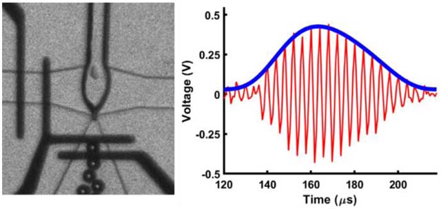
Figure 4.

Raw voltage modulated signals. (A) A 35 μm diameter microbubble produced at 16,500 MB s⁻¹. A 35 μm microbubble is depicted for illustrative purposes but is outside the intended scope of this study. (B) A 15 μm diameter microbubble produced at 70,000 MB s⁻¹. i, ii, iii, iv, and v within the amplitude modulated signal correspond to the microbubble’s position over the electrodes shown in the respective thumbnail images.

Table 1.

Values of coefficients that determine the curves produced by eqns (3) and (4). The curve in the top subplot of Fig. 4C uses the 10 – 17.5 μm microbubble (MB) coefficients. The curves in the bottom subplot of Fig. 4C and Fig. 7B use the normalized value ‘c’ coefficients. The surface plot of Fig. 7A uses the ‘b’ coefficients.

	C1	C2	C3	C4
10 μm MB	−3.743 × 10−3	8.116 × 10−3	1.779 × 10−2	2.494 × 10−2
12.5 μm MB	0.3576	0.7609	1.694	2.342
15 μm MB	−8.256	−17.54	−42.39	−55.32
17.5 μm MB	58.57	1.265 × 102	3.382 × 102	4.177 × 102
normalized value	−5.437 × 10−5	5.144 × 10−3	−0.1183	0.8366
	b1	b2	b3	b4
value	33.224	−1.1904 × 10−4	−7.4976 × 10−2	6.223 × 10−12

3.1c. Counting microbubbles

The conventional approach for establishing production rates of microbubbles produced by microfluidic devices involves measuring the time elapsed between sequential microbubble break off events as observed using high speed microscopy^39,53–55. Determining microbubble production rates using this approach is tedious, typically lacks fine resolution and is susceptible to temporal sampling artifacts (e.g. aliasing). Using the electrical detection strategy presented, if each electrical voltage perturbation is distinguishable, then the production rate can be established with greater ease, accuracy and confidence. In our studies, data of captured production rates were corroborated with optically determined production rates. The optically determined production rates are compared to the electrically determined production rates (R² = 0.98) in ESI† S3A. The residuals are plotted in ESI† S3B. So long as the impedance magnitude perturbations give rise to signals distinguishable from the electrical noise floor, the electrically determined rate is considered to be fault-free and consistent with the decades of experience with Coulter counters which have long been considered the “gold standard” for this measurement. None of the FFMDs that we tested produced microbubbles too small to be counted reliably. However, in rare faulty operation conditions⁵⁸, it is possible to observe pairing of large and small bubbles. In these cases, the small bubbles will probably not be detectable.

3.2. Detection of multiple microbubbles

3.2a. FEA results

The impedance magnitude curve for a train of four microbubbles of a given diameter and centreto-centre spacing is presented in Fig. 5A, in conjunction with a schematic explaining the centreto-centre spacing variable. Fig. 5B illustrates how the relative and absolute impedance magnitude changes as a function of spacing between consecutive 15 μm diameter microbubbles. The absolute impedance magnitude increases as consecutive 15 μm diameter microbubbles simultaneously traverse the detection region and, consequently, the signal is perceived as a larger microbubble rather than two smaller microbubbles. As shown in Fig. 5C, the constructive interference between two microbubbles simultaneously passing through the detection region consumes greater than 90% of the sensors dynamic range as the centre-to-centre spacing approaches the diameter of the microbubbles.

Figure 5.

Multiple microbubble FEA investigation. (A) Top – Schematic detailing derivation of centre-to-centre (C2C) distance between microbubbles. Bottom – representative result of 15 μm microbubbles with 47.5 μm centre-to-centre spacing between each microbubble. (B) Simulation results from multiple microbubbles of a given diameter passing over the electrodes highlight the signal dependence on centre-to-centre spacing between microbubbles. (C) Top – Simulation results indicating the impact of microbubble centre-to-centre spacing for different diameter microbubbles. Bottom – Normalized curve depicting the simulated data follows a cubic relationship.

In these instances, the relative change in measured impedance magnitude attributable to each individual microbubble is attenuated, and the formula for determining electrical diameter in the case of a single microbubble is no longer valid (eqn (1)). However, as shown in Figure 5C, when the relative impedance magnitude curves for each microbubble diameter are normalized to their maximum value, a cubic relationship exists (red curve) between the relative scaling effect and the centre-to-centre distance (R² = 0.99). Critically, the scaling effect is independent of microbubble diameter, which means eqn (1) can be modified by a scaling correction factor that accounts for the constructive interference caused by the presence of multiple microbubbles within the detection region. Thus, a corrected electrical diameter may be determined by the following equation:

$$D_{E,corrected}=CF(x)G_{AVG}\text{Δ}{V}^{1/3},$$ (2)

where CF(x),the corrective term, is a function of x,the centre-to-centre spacing, and is derived data relating the normalized impedance magnitude to the centre-to-centre distance between microbubbles, as shown by the red curve in Fig. 5C. CF(x)takes the form of,

$$CF(x)=c_1{x}^3+c_2{x}^2+c_{3}x+c_4,$$ (3)

where values for c₁, c₂, c₃, and c₄ can be found in table 1 and fit the simulated curves in Fig. 5C. Values of C(x) range between 1 and 20 (unitless) and are valid for production rates between 0 and 3.25×10⁵ MB s⁻¹. The correction factor and compensation method presented in this work is analogous to a compensation method correcting for the positional dependence of particles traversing a channel with coplanar electrodes proposed by Errico et al. This regression was described in the ‘calibration method’ section of the methods (denoted as ‘2.’ in Fig. 2) and will be further characterized in section 3.2c.

3.2b. Experimental results

The FFMD was operated at varying gas pressures and liquid flow rates required to produce microbubbles of 10, 12.5, 15, and 17.5 μm diameters at different production rates. Fig. 6 illustrates how the voltage modulation for a given microbubble diameter changes as a function of the centre-to-centre distance between successively produced microbubbles. In Fig. 6, each circular datum point represents the average measured voltage modulation for a train of microbubbles as a function of the optically determined centre-to-centre distance within the train. Note that each datum point represents a distinct set of gas and liquid operating parameters for the device and that experimental data was taken such that measured diameters were within ±0.5 μm of the stated diameter. The experimental results qualitatively agree with the FEA simulations discussed 3.2a, in that the relative modulation in voltage is significantly attenuated at production rates in which the distance between successively produced microbubbles is less than the end-to-end distance of the detection region. The majority of device operation occurs in this regime, at production rates greater than approximately 1 × 10⁴ MB s⁻¹. Below that production rate, microbubble production tends to be characterized by doublet or triplet production that this device is currently not equipped to handle.

Figure 6.

FEA simulations (solid lines) with overlaid experimental observations (open circles) of voltage modulation with varying centre-to-centre distances for (Top Left) 17.5 μm microbubbles, (Top Right) 15 μm microbubbles, (Bottom Left) 12.5 μm microbubbles and (Bottom Right) 10 μm microbubbles.

To quantitatively compare the experimental results to the FEA simulations, the FEA simulations were extended to include PSpice circuit simulations that evaluated the magnitude of the voltage modulation for microbubbles passing through the detection region using the amplification electronics incorporated within the experimental system. Results from the FEA simulations were used as input parameters. The solid curves in Fig. 6 are simulated results representing the magnitude of voltage modulation for microbubbles of a given diameter as a function of the centre-to-centre distance between sequentially produced microbubbles. As shown, empirically measured electrical estimates of 17.5, 15, 12.5 and 10 μm diameter microbubbles produced at varying production rates match the FEA generated curves for each optically measured microbubble diameter to coefficients of determination, (R² = 0.954, 0.911, 0.907 and 0.773, respectively (Fig. 6)).

3.2c. Compensation method

To accurately size microbubbles when more than one is located within the sensing region, the corrective scaling factor, CF(x), described in 3.2a must be determined from the electrically measured voltage traces. For a given set of operating conditions, CF(x) of eqn (2) is determined through a two-step process.

First, the production rate is measured from the electrical signal using a peak detection algorithm. The electrically derived production rate (PR) and the fluid flow rate (FFR) are then mapped to a corresponding centre-to-centre (C2C) distance by the three-dimensional surface fit, as shown in Fig. 7A. As expected, the centre-to-centre distance decreases as the production rate increases. Asymptotic behaviour is observed near a centre-to-centre distance of 10 μm as the production rate increases beyond 2 × 10⁵ MB s⁻¹. This behaviour accounts for the physically limiting case that two sequential microbubbles cannot have a centre-to-centre distance smaller than their diameter. A multiple linear regression (mesh surface) was fitted to the data and to establish the relationship between the centre-to-centre distance, electrically measured production rate and fluid flow rate. The equation takes the form,

$$C2C(PR,FFR)=b_1+b_{2}PR+b_{3}FFR+b_{4}P{R}^{2}FFR,$$ (4)

where values of b₁,b₂,b₃ and b₄ can be found in table 1. This regression is used in the device calibration method, described in 3.2c. The coefficient of determination for this fit was R² = 0.92.

Figure 7.

Description of the compensation strategy. (i) First, the production rate is taken from electrically acquired data and is applied to a cubic polynomial equation that relates production rate to centre-tocentre distance between microbubbles. (ii) After a centre-to-centre distance is derived, the value is used to calculate the correction factor to be applied using a cubic polynomial relationship between the centre-to-centre distance and correction factor. 10 μm and 12.5 μm microbubble data include centre-tocentre distances between 12.5 μm and 47.5 μm at 5 μm increments. 15 μm and 17.5 μm microbubble data include centre-to-centre distances between 17.5 μm and 47.5 μm at 5 μm increments.

Second, this estimate of the centre-to-centre distance is then mapped to CF(x) using the red curve-fit in Fig. 7B, which relates CF(x) to the centre-to-centre distance using FEA simulated data. Eqn (3) becomes,

$$CF(C2C)=c_{1}C2C^3+c_{2}C2C^2+c_{3}C2C+c_4,$$ (5)

Note that the first step of this calibration process is device-specific, as the relationship between production rate and centre-to-centre distance is based on empirically measured data for a single device. We envisage that in a tight, quality-controlled, production setting, the calibration results will be generalizable over the device population. The second step is generalizable to all devices of a particular sensing geometry because it is determined from FEA simulations.

This calibration strategy was used to account for the reduced voltage modulation as multiple microbubbles passed through the sensing region. The black curve in Fig. 8A shows the expected voltage modulation for single microbubbles of varying diameters passing through the sensing region, as simulated by the combined FEA and PSpice model. The blue data points are empirically measured voltage modulations from microbubbles passing through the sensing region and their accompanying optically-determined diameters. Prior to calibration, there exists a significant error between the expected voltage modulation (eqn (1)) and the experimentally determined voltage modulation. However, when the experimental data were corrected for the centre-to-centre distance between successively produced microbubbles, inversely the production rate, the microbubble data tightly follows a cubic approximation as depicted in Fig. 8B. The application of CF(x) in eqn (2) describes the attenuation phenomenon and corrects the observed voltage modulation for scaling related to reduced centre-to-centre distances.

Figure 8.

Plot showing the correlation between the microbubble (MB) diameter and the magnitude of the impedance magnitude change. The points along the curve were obtained from PSpice circuit simulations for microbubbles of different diameters. The data points were obtained from acquisitions of electrical data varying microbubble production rates and diameters. Error bars are not shown for voltage because the variance in voltage is so small that the error bars do not appear conspicuously in the figure. (A) Raw data. (B) Corrected data.

3.3. Estimation of microbubble diameter

After validating the compensation strategy introduced in eqns (1) and (2) and establishing a correction factor that scales with production rate, microbubbles were fabricated at different diameters and production rates and electrical and optical data were simultaneously acquired. Fig. 9 illustrates electrically determined microbubble diameter versus optically determined microbubble diameter. The electrically observed diameters were corrected using the electrically determined microbubble production rate as an input to the compensation method, as described in 3.2c. The figure illustrates that microbubbles of similar diameters and different productions rates still result in electrically determined diameters of an equivalent size, which was not achieved prior to the regression-based calibration operation, and demonstrates the agreement between the optical and electrical methods of measurement. A tight grouping along the diagonal line y = x denotes excellent agreement, R² = 0.91, between the two methods of microbubble detection. A coefficient of determination, R² = 0.93, follows the line y = 0.91x + 1.04. A plot of the residual values comparing optically determined diameter to the electrically determined diameter is reported in ESI† S4.

Figure 9.

Comparison of methods to determine microbubble (MB) diameter. Optically determined microbubble diameter spans the x axis and electrically determined microbubble diameter the y axis. The black line is y=x and data points on that line demonstrates excellent agreement.

4. Discussion

4.1. Device Performance

The results of this study demonstrate a μCPC integrated within the expanding nozzle of an FFMD capable of counting microbubbles up to 3.25 × 10⁵ MB s⁻¹ at sizes down to approximately 8 μm in diameter; parameters that meet, or exceed, projected needs relevant to our application. Measured noise indicates that the μCPC is capable of sensing microbubbles as small as 2.5 μm in diameter; however, only microbubbles of ≥ 8 μm were investigated in this study. To our knowledge, this is the first demonstration of sequential production and characterization of microbubbles by a μCPC integrated within the expanding nozzle of a flow focusing device at high throughput (> 1 × 10⁴ MB s⁻¹). This strategy achieves a non-optical method of characterization that is low cost and portable for the analysis of benchtop FFMD microbubble production. The method has the potential to benefit in vivo research of FFMDs previously limited due to the constraints of high-speed optical microscopy. A primary example where this technology can be deployed is as a quality control system on a catheter tip measuring microbubbles administered for therapeutic benefit in various blood clot dissolution settings⁴⁰. Further, this strategy extends to research involving the administration of liquid micro-droplets or other more exotic particles produced using an FFMD in which a material phase contrast in impedance magnitude is present. Ultimately, this strategy may prove clinically useful for sonothrombolysis in a blood clot dissolution setting. It achieves a quality control and safety assurance solution necessary for real-time control and verification of generated material as it is administered to patients.

This novel μCPC design benefits from unique features of FFMD-produced microbubbles. Foremost, when producing microbubbles at a high production rate, the electrical signals within the detection region from individual microbubbles superimpose to produce a combined signal that resembles that of a larger microbubble. However, as demonstrated by the analysis, individual microbubble signals were decoded from a signal featuring multiple microbubbles simultaneously within the detection region by detecting the relative, not absolute, change in signal. This compensation strategy is enabled by the high degree of similarity between sequentially produced monodisperse microbubbles within FFMDs. Under controlled conditions, the gas pinch-off mechanism at the nozzle results in the continuous generation of substantially equivalent microbubbles separated by equal distances. The data (Fig. 8B) support results from Bernabini et al., who reported a cubic polynomial change in the impedance magnitude with respect to particles of different radii²⁵. The finding is expected as the volume of a sphere is governed by the third power of the radius. Conversely, conventional μCPC analysis of heterogeneous particles requires significant dilution of the particle-containing phase to prevent the occurrence of two or more multiply-sized particles simultaneously within the detection region. Thus, as a result of needing to dilute the particle-containing solution, high throughputs (> 1 × 10⁴ particles s⁻¹) are seldom achieved.

4.2. Limitations

Coplanar electrodes offer a simplified fabrication process relative to top-and-bottom electrodes and are commonly used for the fabrication of μCPCs. While coplanar electrode devices have been predominant in the literature, they suffer from decreased sensitivity due to a necessarily larger detection region than the top-and-bottom electrode configuration⁷. Additionally, nonuniform current in the detection region causes an impedance magnitude modulation dependent on the height of the particle in channel. Spencer et al. recently demonstrated a post-processing algorithm to correct for height dependence using coplanar electrodes²⁹.

At higher production rates, multiple microbubbles enter the detection region simultaneously and consequently decrease the relative amplitude modulation by interfering with each microbubble’s measurement. However, this may be addressed by using a compensation strategy that corrects for the production rate or, conversely, the centre-to-centre distance between successively produced microbubbles. A complementary component to further enhance agreement in detection methods would include compiling a library of data on the device including liquid flow rates and gas pressures to produce microbubbles of certain diameters and production rates. Wang et al. constructed a library of microbubble production parameters using a FFMD that preceded this device⁵⁸. Liquid phase flow rates and gas pressures were varied to encompass the various sizes and production rates that were achieved using the FFMD. Using the library of data similarly, with a given liquid phase flow rate, gas pressure, and production rate (electrically detected), a microbubble size could then be extracted. The study investigated various production regimes, including doublet and triplet production of microbubbles that yielded polydisperse populations⁵⁸. The study presented here is constrained to monodisperse microbubbles produced sequentially. Since the proposed method cannot directly determine the presence of doublet or triplet formation, it is necessary to ensure that the operating parameters are outside of those consistent with the potential for doublet and triplet formation. In practice, this condition is easily met.

An additional limitation is that the FEA simulations maintain a constant spacing between the microbubbles as they flow through the expanding nozzle, which does not account for the reduction in speed out of the nozzle of microbubble approximately 40–50 μm downstream of the nozzle. The observed decrease in velocity by the microbubble occurs while it is within the detection region, specifically over the ground electrode, and thus still imposes and consequently interferes with the modulated electrical signal detected. It is possible to mitigate this effect by shortening the width of the coplanar electrodes, thereby decreasing the length of the detection region. Interestingly, simulation results predict detection does not improve by an appreciable amount due to the change in coplanar channel geometry (results not shown); however, the pulse width does narrow as expected. One would expect an enhanced ability to distinguish production rates < 3.25 × 10⁵ MB s⁻¹ and, consequently, a decreased dependence on applying a production rate correction factor.

5. Conclusion

In the present study, a benchtop FFMD with an integrated μCPC was fabricated and demonstrated in situ production and characterization of microbubbles; however, we envision broad utilization for characterization of liquid micro-droplets as well. The μCPC detected microbubbles using coplanar electrodes that were electrically excited with an AC signal. The passage of microbubbles within the detection region and confined by the electrodes creates a modulation in the impedance magnitude between the two electrodes that was measurable. Simulations informed the design of the integrated electrode detection region, established the theoretical performance of the device and were validated by experimental data. Single microbubble simulations established the maximum impedance magnitude modulation within the detection region. Multi-microbubble simulations established the anticipated impedance magnitude modulation for microbubbles of a given diameter at variable production rates and established a relationship that was used to relate the optically determined centre-to-centre distance between successively produced microbubbles to a correction factor. Further, a calibration method was established that accounted for the interference resulting from the presence of multiple microbubbles in the detection region simultaneously. Experimental detection of microbubble populations of different sizes (8 – 20 μm diameter) and production rates (< 3.25 × 10⁵ MB s⁻¹) were achieved and compared to simulated data and optical detection techniques. Results demonstrate excellent agreement (R² = 0.91) between electrical and optical detection. In conclusion, the system counts and measures the diameter of microbubbles at production rates (< 3.25 × 10⁵ MB s⁻¹) and diameters (8 – 20 μm) that meet, or exceed, projected needs relevant to our application.

References

- 1.Zhang H, Chon CH, Pan X and Li D, Microfluid. Nanofluid., 2009, 7, 739–749. [DOI] [PMC free article] [PubMed] [Google Scholar]
- 2.Coulter WH, US Patent 2,656,508, 1953. [Google Scholar]
- 3.DeBlois RW and Bean CP, Rev. Sci. Instrum., 1970, 41, 909–916. [Google Scholar]
- 4.DeBlois RW and Wesley RK, J. Virol., 1977, 23, 227–233. [DOI] [PMC free article] [PubMed] [Google Scholar]
- 5.Anderson JR, Chiu DT, Wu H, Schueller OJ and Whitesides GM, Electrophoresis, 2000, 21, 27–40. [DOI] [PubMed] [Google Scholar]
- 6.Sia SK and Whitesides GM, Electrophoresis, 2003, 24, 3563–3576. [DOI] [PubMed] [Google Scholar]
- 7.Gawad S, Schild L and Renaud P, Lab Chip, 2001, 1, 76–82. [DOI] [PubMed] [Google Scholar]
- 8.Rodriguez-Trujillo R, Mills CA, Samitier J and Gomila G, Microfluid. Nanofluid., 2006, 3, 171–176. [Google Scholar]
- 9.Jagtiani AV, Zhe J, Hu J and Carletta J, Meas. Sci. Technol., 2006, 17, 1706–1714. [Google Scholar]
- 10.Saleh OA and Sohn LL, Rev. Sci. Instrum., 2001, 72,4449–4451. [Google Scholar]
- 11.Lee G-B, Lin C-H and Chang G-L, Sens. Actuators A Phys., 2003, 103, 165–170. [Google Scholar]
- 12.Pamme N, Koyama R and Manz A, Lab Chip, 2003, 3, 187–192. [DOI] [PubMed] [Google Scholar]
- 13.Xiang Q, Xuan X, Xu B and Li D, Instrum. Sci. Technol., 2005, 33, 597–607. [Google Scholar]
- 14.Gawad S, Cheung K, Seger U, Bertsch A and Renaud P, Lab Chip, 2004, 4, 241–251. [DOI] [PubMed] [Google Scholar]
- 15.Cheung K, Gawad S and Renaud P, Cytometry Part A, 2005, 65, 124–132. [DOI] [PubMed] [Google Scholar]
- 16.Sohn LL, Saleh OA, Facer GR, Beavis AJ, Allan RS and Notterman DA, Proc. Natl. Acad. Sci. U. S. A, 2000, 97, 10687–10690. [DOI] [PMC free article] [PubMed] [Google Scholar]
- 17.Murali S, Xia X, Jagtiani AV, Carletta J and Zhe J, Smart Mater. Struct., 2009, 18, 037001. [Google Scholar]
- 18.Bayley H and Martin CR, Chem. Rev., 2000, 100, 2575–2594. [DOI] [PubMed] [Google Scholar]
- 19.Carbonaro A and Sohn LL, Lab Chip, 2005, 5, 1155–1160. [DOI] [PubMed] [Google Scholar]
- 20.Kasianowicz JJ, Brandin E, Branton D and Deamer DW, Proc. Natl. Acad. Sci. U. S. A, 1996, 93, 13770–13773. [DOI] [PMC free article] [PubMed] [Google Scholar]
- 21.Niu X, Zhang M, Peng S, Wen W and Sheng P, Biomicrofluidics, 2007, 1, 044101. [DOI] [PMC free article] [PubMed] [Google Scholar]
- 22.Cheung KC, Di Berardino M, Schade-Kampmann G, Hebeisen M, Pierzchalski A, Bocsi J, Mittag A and Tarnok A, Cytometry Part A, 2010, 77,648–666. [DOI] [PubMed] [Google Scholar]
- 23.Kummrow A, Theisen J, Frankowski M, Tuchscheerer A, Yildirim H, Brattke K, Schmidt M and Neukammer J, Lab Chip, 2009, 9, 972–981. [DOI] [PubMed] [Google Scholar]
- 24.Simon P, Frankowski M, Bock N and Neukammer J, Lab Chip, 2016, 16, 2326–2338. [DOI] [PubMed] [Google Scholar]
- 25.Bernabini C, Holmes D and Morgan H, Lab Chip, 2011, 11, 407–412. (33) [DOI] [PubMed] [Google Scholar]
- 26.Lee G-B, Hung C-I, Ke B-J, Huang G-R, Hwei B-H and Lai H-F, J. Fluids Eng., 2001, 123, 672–679. [Google Scholar]
- 27.Nieuwenhuis JH, Kohl F, Bastemeijer J, Sarro PM and Vellekoop MJ, Sens. Actuators B. Chem., 2004, 102, 44–50. [Google Scholar]
- 28.Wu X, Kang Y, Wang Y-N, Xu D, Li D and Li D, Electrophoresis, 2008, 29, 2754–2759. [DOI] [PubMed] [Google Scholar]
- 29.Spencer D, Caselli F, Bisegna P and Morgan H, Lab Chip, 2016, 16, 2467–2473. [DOI] [PubMed] [Google Scholar]
- 30.Gawad S, Sun T, Green NG and Morgan H, Rev. Sci. Instrum., 2007, 78, 054301. [DOI] [PubMed] [Google Scholar]
- 31.Sun T, van Berkel C, Green NG and Morgan H, Microfluid. Nanofluid., 2009, 6, 179–187. [Google Scholar]
- 32.Xie P, Cao X, Lin Z, Talukder N, Emaminejad S and Javanmard M, Sens. Actuators B. Chem., 2017, 241, 672–680. [Google Scholar]
- 33.Song Y, Yang J, Pan X and Li D, Electrophoresis, 2015, 36, 495–501. [DOI] [PubMed] [Google Scholar]
- 34.Wood DK, Oh S-H, Lee S-H, Soh HT and Cleland AN, Appl. Phys. Lett., 2005, 87, 184106. [Google Scholar]
- 35.Fraikin J-L, Teesalu T, McKenney CM, Ruoslahti E and Cleland AN, Nat. Nanotechnol., 2011, 6, 308–313. [DOI] [PubMed] [Google Scholar]
- 36.Dong T and Barbosa C, Sensors, 2015, 15, 2694–2708. [DOI] [PMC free article] [PubMed] [Google Scholar]
- 37.Yakdi NE, Huet F and Ngo K, Sens. Actuators B. Chem., 2016, 236, 794–804. [Google Scholar]
- 38.Garstecki P, Fuerstman MJ, Stone HA and Whitesides GM, Lab Chip, 2006, 6, 437–446. [DOI] [PubMed] [Google Scholar]
- 39.Hettiarachchi K, Talu E, Longo ML, Dayton PA and Lee AP, Lab Chip, 2007, 7, 463–468. [DOI] [PMC free article] [PubMed] [Google Scholar]
- 40.Dixon AJ, Rickel JMR, Shin BD, Klibanov AL and Hossack JA, Ann Biomed Eng., 2018, 46, 10.1007/s10439-017-1965-7. [DOI] [PMC free article] [PubMed] [Google Scholar]
- 41.Keller MW, Feinstein SB and Watson DD, Am. Heart J., 1987, 114, 570–575. [DOI] [PubMed] [Google Scholar]
- 42.Wei K, Jayaweera AR, Firoozan S, Linka A, Skyba DM and Kaul S, Circulation, 1998, 97, 473–483. [DOI] [PubMed] [Google Scholar]
- 43.Bardin D , Martz TD, Sheeran PS, Shih R, Dayton PA, and Lee AP, Lab Chip, 2011, 11, 3990–3998. [DOI] [PMC free article] [PubMed] [Google Scholar]
- 44.Martz TD, Sheeran PS, Bardin D, Lee AP, and Dayton PA, Ultrasound Med.Biol, 2011, 37, 1952–1957. [DOI] [PMC free article] [PubMed] [Google Scholar]
- 45.Prentice P, Cuschieri A, Dholakia K, Prausnitz M, and Campbell P, Nat. Phys., 2005, 1, 107–110. [Google Scholar]
- 46.van Wamel A, Kooiman K, Harteveld M, Emmer M, ten Cate FJ, Versluis M, and de Jong N, J. Control. Release, 2006, 112,149–155. [DOI] [PubMed] [Google Scholar]
- 47.Dixon AJ, Dhanaliwala AH, Chen JL, and Hossack JA, Ultrasound Med. Biol, 2013. 39, 1267–1276. [DOI] [PMC free article] [PubMed] [Google Scholar]
- 48.Alexandrov AV, Molina CA, Grotta JC, Garami Z, Ford SR, Alvarez-Sabin J, et al. , New Engl. J. Med., 2004, 351, 2170–2178. [DOI] [PubMed] [Google Scholar]
- 49.Molina CA, Ribo M, Rubiera M, Montaner J, Santamarina E, Delgado-Mederos R, et al. , Stroke, 2006, 37,425–429. [DOI] [PubMed] [Google Scholar]
- 50.Berkhemer OA, Fransen PSS, Beumer D, van den Berg LA, Lingsma HF, Yoo AJ, et al. , New Engl. J. Med., 2015, 372, 11–20.25517348 [Google Scholar]
- 51.Fritz TA, Unger EC, Sutherland G and Sahn D, Invest. Radiol., 1997, 32, 735–740. [DOI] [PubMed] [Google Scholar]
- 52.Klibanov AL, Contrast Agents II, 2002, 73–106. [Google Scholar]
- 53.Gañán-Calvo AM and Gordillo JM, Phys. Rev. Lett., 2001, 87, 274501. [DOI] [PubMed] [Google Scholar]
- 54.Castro-Hernández E, van Hoeve W, Lohse D and Gordillo JM, Lab Chip, 2011, 11,2023–2029. [DOI] [PubMed] [Google Scholar]
- 55.Garstecki P, Gitlin I, DiLuzio W, Whitesides GM, Kumacheva E and Stone HA, Appl. Phys. Lett., 2004, 85, 2649–2651. [Google Scholar]
- 56.Talu E, Hettiarachchi K, Powell RL, Lee AP, Dayton PA and Longo ML, Langmuir, 2008, 24, 1745–1749. [DOI] [PMC free article] [PubMed] [Google Scholar]
- 57.Dhanaliwala AH, Dixon AJ, Lin D, Chen JL, Klibanov AL, and Hossack JA, Biomed. Microdevices, 2015, 17:23, DOI: 10.1007/s10544-014-9914-9. [DOI] [PubMed] [Google Scholar]
- 58.Wang S, Dhanaliwala AH, Chen JL and Hossack JA, Biomicrofluidics, 2013, 7, 014103. [DOI] [PMC free article] [PubMed] [Google Scholar]
- 59.Dhanaliwala AH, Chen JL, Wang S and Hossack JA, Microfluid. Nanofluid, 2012, 14, 457–467. [DOI] [PMC free article] [PubMed] [Google Scholar]
- 60.Errico V, De Ninno A, Bertani FR, Businaro L, Bisegna P and Caselli F, Sens. Actuators B. Chem., 2017, 247, 580–586. [Google Scholar]
Associated Data
This section collects any data citations, data availability statements, or supplementary materials included in this article.