Multiple time-frequency curve extraction Matlab code and its application to automatic bearing fault diagnosis under time-varying speed conditions

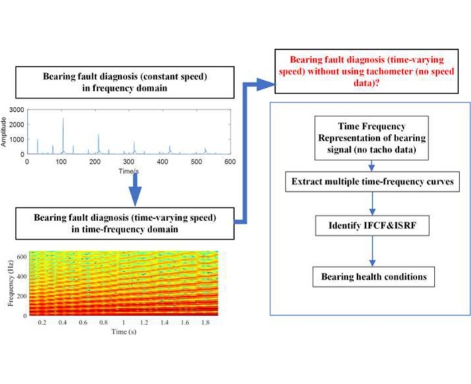
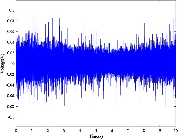
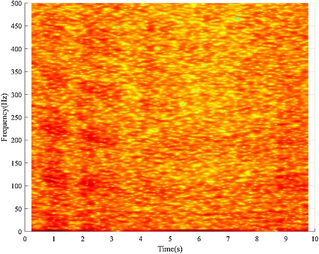
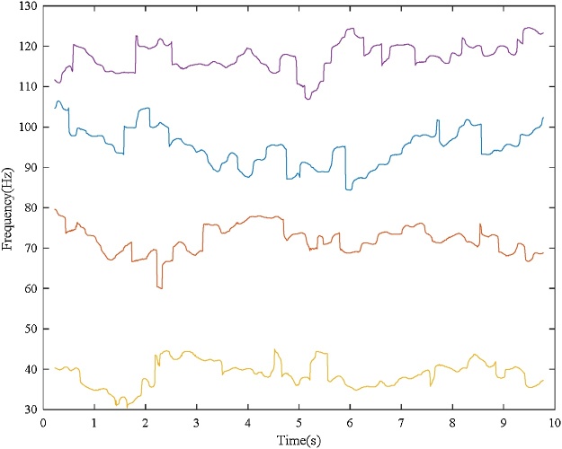
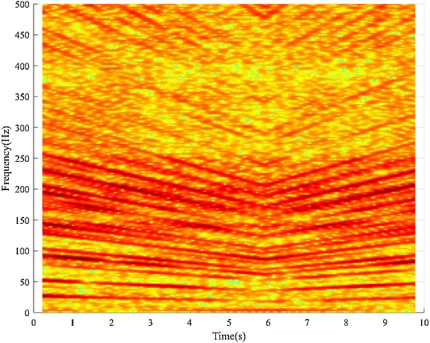
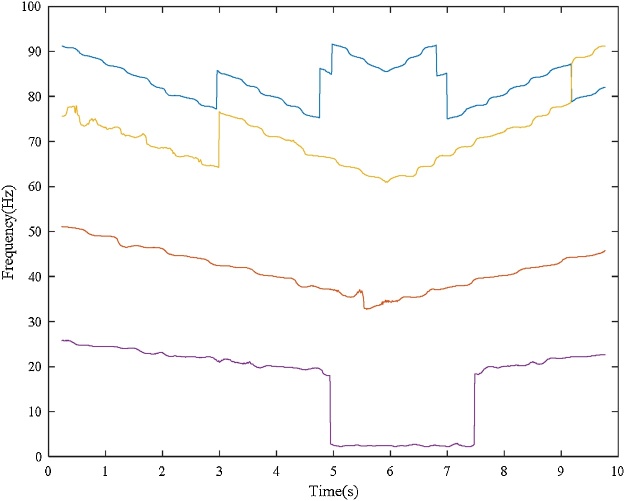
Graphical abstract

Abstract

Vibration signal analysis is an important technique for bearing fault diagnosis. For bearings operating under constant rotational speed, faults can be diagnosed in the frequency domain since each type of fault has a specific Fault Characteristic Frequency (FCF), which is proportional to the shaft rotational speed. However, bearings often operate under time-varying speed conditions. Additionally, the measurement of the time-varying rotational speed requires instruments, such as tachometers, which leads to extra cost and installation. With the development of time-frequency analysis, the time-varying FCFs manifest as curves in the Time-Frequency Representation (TFR). It has been shown that extracting multiple time-frequency curves from the TFR and then identifying the Instantaneous Fault Characteristic Frequency (IFCF) and Instantaneous Shaft Rotational Frequency (ISRF), bearing faults can be automatically diagnosed under time-varying speed conditions without using tachometers. However, the existing method used to identify the IFCF and the ISRF may lead to inaccurate results. In this study, the complete MATLAB© codes and a more reliable approach to use Multiple Time-Frequency Curve Extraction (MTFCE) for automatic bearing fault diagnosis under time-varying speed conditions are presented.

• •A Multiple time-frequency curve extraction (MTFCE) Matlab code is presented to extract multiple curves from the TFR.
• •Custom Matlab code for automatic bearing fault diagnosis under time-varying speed conditions without using tachometer data via the MTFCE is given and explained.
• •A new parameter, the allowable variance of the curve-to-curve ratio, is proposed to identify the IFCF and ISRF more reliably.

Nomenclature

X(τ, f)

TFR of signal x(t)

τ

Variable referring to time

f

Variable referring to frequency

f_p(τ)

Extracted time-frequency curve

f_up(τ)

Upper boundary of a curve

f_down(τ)

Lower boundary of a curve

N_p(τ_n)

Number of peaks at time τn in the TFR

v_m(τ_n)

Frequency of the mth peak at τn

Q_m(τ_n)

TFR amplitude of the mth peak at τn

m_c(τ_n)

Index of the extracted peak at τn

q(m, τ_n)

Vector indicating liked peaks between τn and τn-1

U(m, τ_n)

Intermediate vector contributing to the optimization

N_c

Number of T-F curves to extract

isrf

Estimated instantaneous shaft rotational frequency

fcci

Fault characteristic coefficient of inner race fault

fcco

Fault characteristic coefficient of outer race fault

er_i

Allowed error of |average_ratio-fcci|/fcci

er_o

Allowed error of |average_ratio-fcco|/fcco

var_i

Allowed variance of curve-to-curve ratio of inner race fault

var_o

Allowed variance of curve-to-curve ratio of outer race fault

ifcf

Identified instantaneous fault characteristic frequency

Specifications Table

Subject Area:	Engineering
More specific subject area:	Vibration, signal processing, machinery condition monitoring
Method name:	Automatic bearing fault diagnosis under time-varying speed conditions via multiple time-frequency curve extraction
Name and reference of original method:	Huang, Huan, Natalie Baddour, and Ming Liang. "Bearing fault diagnosis under unknown time-varying rotational speed conditions via multiple time-frequency curve extraction." Journal of Sound and Vibration 414 (2018): 43-60. Iatsenko, Dmytro, Peter VE McClintock, and Aneta Stefanovska. "Extraction of instantaneous frequencies from ridges in time-frequency representations of signals." Signal Processing 125 (2016): 290-303.
Resource availability:	Matlab R2016b, Datahttps://doi.org/10.17632/v43hmbwxpm.1

Introduction

Bearing fault diagnosis is an important means to prevent the breakdown of rotating machines. Vibration and acoustic signal analyses are commonly used techniques for bearing fault diagnosis since the local defect at a certain location induces a specific Fault Characteristic Frequency (FCF) to the signal and the FCF is proportional to the rotational frequency [1]. Based on this knowledge, bearing fault diagnosis under constant rotational speed condition has been widely investigated [[2], [3], [4], [5], [6], [7], [8]]. However, bearings often operate under time-varying speed conditions which results in a time-varying FCF. Under such circumstance, methods used for the case of constant speed are not applicable. Therefore, investigations of bearing fault diagnosis under time-varying speed conditions are critical for industrial applications.

Various methods have proposed for bearing fault diagnosis under time-varying speed conditions, including methods based on signal resampling [[9], [10], [11]], methods based on machine learning [12,13], and methods based on time-frequency analysis [14,15]. Resampling the bearing vibration signal according to the time-varying rotational speed can convert the time-varying FCF into a constant Fault Characteristic Order (FCO) [9]. With the FCO, bearing faults can then be diagnosed similarly to the case of constant speed. However, the accuracy of signal resampling is limited by many factors such as interpolation methods. Also, additional instruments are required to measure the rotational speed. Machine learning methods can be used to automatically diagnose bearing faults without the acquisition of the rotational speed and signal resampling [12,13]. However, numerous data are required to train the method-related parameter or classifier. Time-frequency analysis techniques, such as Short-Time Fourier Transform (STFT), can be used to present the Instantaneous Fault Characteristic Frequency (IFCF) as a curve in the Time-Frequency Representation (TFR) [14]. Additionally, the TFR can be used to estimate the time-varying rotational speed or Instantaneous Shaft Rotational Frequency (ISRF). Therefore, bearing fault diagnosis methods based on the time-frequency analysis is free from signal resampling and does not require numerous data for training. However, for automatic bearing fault diagnosis, the IFCF and the ISRF need to be extracted from the TFR.

Multiple Time-Frequency Curve Extraction (MTFCE) algorithm is a newly proposed method which can be used to extract time-frequency curves from the TFR of a signal [[16], [17], [18]]. With the MTFCE algorithm, multiple time-frequency curves can be extracted from the TFR of bearing vibration signal. Bearing faults can be automatically diagnosed if the IFCF and ISRF are recognized from the extracted time-frequency curves. In [16], the extracted time-frequency curves are identified as the IFCF and the ISRF by calculating the average frequency ratio of two curves and comparing the average ratio to the Fault Characteristic Coefficient (FCC) of each fault types. The FCC is the ratio of the FCF to the rotational frequency, which remains constant under time-varying speed conditions. Therefore, the average ratio of the IFCF to the ISRF should match the FCC if the bearing is faulty. However, if the bearing is healthy, it is possible that the average ratio of two randomly extracted curves matches the FCC yet either of the extracted curve is the IFCF or the ISRF. This will lead to a false result that a healthy bearing is diagnosed as faulty. Therefore, the average ratio of two curves is not sufficient for the identification of the IFCF and the ISRF. In view of this, the variance of the frequency ratio of two curves should also be taken into account to ensure that the frequency ratio at each frequency matches the FCC and not just the average ratio. Such an approach is developed in this paper.

In this paper, Matlab codes of the MTFCE algorithm are provided. Based on the MTFCE algorithm, custom Matlab codes for automatic bearing fault diagnosis under time-varying rotational speed conditions are also provided. In addition, a new parameter, the allowable variance of the curve-to-curve ratio, is proposed to identify the IFCF and ISRF more reliably. With the provided Matlab codes, bearing faults can be diagnosed by simply inputting the bearing vibration signal. The proposed method is free from signal resampling and free from any instrument for measuring the time-varying rotational speed. The effectiveness of the Matlab codes are validated by experimental data collected from bearings operating under time-varying speed conditions.

Method details

In this paper, Matlab codes developed for automatic bearing fault diagnosis under time-varying speed conditions are released, attached in the. zip file. The function bearing_fault_diagnosis.m can be used to automatically diagnose bearing faults via Multiple Time-Frequency Curve Extraction (MTFCE), Instantaneous Shaft Rotational Frequency (ISRF) estimation, Instantaneous Fault Characteristic Frequency (IFCF) identification, etc. Therefore, relevant functions are also included in the. zip file. The function mltcurve.m extracts multiple Time-Frequency (T-F) curves from the Time-Frequency Representation (TFR) of a signal. The function ISRF_estimation.m estimates the ISRF from the extracted multiple T-F curves. The function fault_disgnosis.m identifies the IFCF and diagnoses the bearing fault. Additionally, to compare the estimated ISRF with the measured ISRF, the function encoder.m converts a measured encoder signal into the ISRF and the function compare_isrf calculates the average error of |estimated ISRF-measured ISRF| / measured ISRF. The method is validated with bearing data measured under time-varying speed conditions, which can be found in [19].

In this section, the MTFCE algorithm is explained. In the next section, the method for automatic bearing fault diagnosis is demonstrated. Then, the performance of the method is examined by measured bearing vibration data. Finally, conclusions are drawn based on all the above.

With the development of time-frequency analysis, time-varying frequency characteristics of a signal can be revealed in the time-frequency domain. Time-frequency techniques, such as the Short-Time Fourier Transform (STFT) or wavelet transform, can be used to obtain the Time-Frequency Representation (TFR) of a signal [20]. The time-varying frequencies of the signal appear as T-F curves in the TFR. However, to further analyze or utilize the time-varying frequencies, T-F curves need to be extracted from the TFR.

An algorithm for Multiple Time-Frequency Curve Extraction (MTFCE) is given [16,17], based on a fast path optimization approach. The fast path optimization approach was developed by Iatsenko et al. [21] to reliably extract a single T-F curve from the TFR. The fast path optimization approach employs a support function to optimally extract a T-F curve from the TFR with minimal frequency jumps.

Assuming that the TFR of a signal x(t) is X(τ, f), in which τ is the variable referring to time, f is the variable referring to frequency, then fast path-optimization can be used to extract a T-F curve f_p(τ) from X(τ, f), along with the upper boundary f_up(τ) & lower boundary f_down(τ) of the T-F curve. To explain the approach, the number of peaks at time τ_n in the TFR is denoted as N_p(τ_n), the corresponding frequency of the mth peak as v_m(τ_n), the TFR amplitude of the mth peak as Q_m(τ_n). Peaks at time τ_n can be determined by

$${\nu }_m\left({\tau }_n\right)=f\text{s}\text{.t}\text{.}\left\{\begin{array}{c}\hfill \frac{d\left[X\left({\tau }_n,f\right)\right]}{df}=0\hfill \\ \hfill \frac{d^2\left[X\left({\tau }_n,f\right)\right]}{d{f}^2}<0\hfill \end{array}\right)$$ (1)

If X(τ, f) has a time span [τ₁, τ₂,…, τ_N], the path optimization can be described as

$$\left\{m_c({\tau }_1),\mathrm{...},m_c({\tau }_N)\right\}=\underset{\left\{m_1,\mathrm{...},m_N\right\}}{\arg \max }\sum _{n=1}^{N}F\left[{\tau }_n,Q_{m_n}({\tau }_n),{\nu }_{m_n}({\tau }_n),\left\{{\nu }_{m_1}({\tau }_1),\mathrm{...},{\nu }_{m_N}({\tau }_N)\right\}\right]$$ (2)

where m_c(τ_n) determines the peak to be extracted as the ridge at τ_n, F[] is the chosen support function for the optimization and {m₁,…, m_N} refers to a sequence of the peak numbers along the time span. The fast path optimization is proposed to be only dependent on a finite number of the previous points with the support function [21]

$$F\left[\right]=\left\{\begin{array}{cc}\hfill \log Q_m\left({\tau }_n\right)\hfill & \hfill n=1\hfill \\ \hfill \log Q_m\left({\tau }_n\right)+w_2\left({\nu }_m\left({\tau }_n\right),\text{m}\left[f_d\right],\text{IQR}\left[f_d\right],{\lambda }_2\right)\hfill & \hfill n=2\hfill \\ \hfill \log Q_m\left({\tau }_n\right)+w_2\left({\nu }_m\left({\tau }_n\right),\text{m}\left[f_d\right],\text{IQR}\left[f_d\right],{\lambda }_2\right)+w_1\left({\nu }_m\left({\tau }_n\right)-f_d\left({\tau }_{n-1}\right),\text{m}\left[\Delta f_d\right],\text{IQR}\left[\Delta f_d\right],{\lambda }_1\right)\hfill & \hfill n\ge 3\hfill \end{array}\right)$$ (3)

where

$$w_1\left({\nu }_m\left({\tau }_n\right)-f_d\left({\tau }_{n-1}\right),m\left[\Delta f_d\right],IQR\left[\Delta f_d\right],{\lambda }_1\right)=-{\lambda }_1\left|\frac{{\nu }_{m_n}\left({\tau }_n\right)-f_d\left({\tau }_{n-1}\right)-m\left[\Delta f_d\right]}{IQR\left[\Delta f_d\right]}\right|$$ (4)

$$w_2\left({\nu }_m\left({\tau }_n\right),m\left[f_d\right],IQR\left[f_d\right],{\lambda }_2\right)=-{\lambda }_2\left|\frac{{\nu }_m\left({\tau }_n\right)-m\left[f_d\right]}{IQR\left[f_d\right]}\right|$$ (5)

$$\text{m}[]=\text{per}{\text{c}}_{0.5}[],\text{IQR}[]=\text{per}{\text{c}}_{0.75}[]-\text{per}{\text{c}}_{0.25}[]$$ (6)

where f_d(τ_n-1) is the frequency of the candidate ridge point at τ_n-1, f_d are the frequencies of a series of candidate ridge points in history [τ₁,…, τ_n-1], Δf_d is the derivative of f_d, m[] refers to the median of a series, IQR is the interquartile range, perc_p denotes the pth quantile of a series, and λ₁ and λ₂ are penalty factors which can be taken as 1. Weight functions w₁() and w₂() are employed to suppress the atypical variations of the ridge frequency’s value and derivative, respectively. With the support function, the fast path optimization can be used to effectively extract the T-F curve from the TFR of a signal with minimum/ without frequency jumps.

The optimization problem can be solved as [21]:

$$\begin{array}{l}forn=1,\mathrm{...},N\text{,}m=1,\mathrm{...},N_p\left({\tau }_n\right)\text{and}k=1,\mathrm{...},N_p\left({\tau }_{n-1}\right)\\ q\left(m,{\tau }_n\right)=\underset{k}{\arg \max }\left\{F\left[Q_m\left({\tau }_n\right),{\nu }_m\left({\tau }_n\right),{\nu }_k\left({\tau }_{n-1}\right)\right]+U\left(k,{\tau }_{n-1}\right)\right\},n>1\\ U\left(m,{\tau }_n\right)=\left\{\begin{array}{cc}\hfill F\left[Q_m\left({\tau }_n\right),{\nu }_m\left({\tau }_n\right),{\nu }_m\left({\tau }_n\right)\right]\hfill & \hfill n=1\hfill \\ \hfill F\left[Q_m\left({\tau }_n\right),{\nu }_m\left({\tau }_n\right),{\nu }_{q\left(m,{\tau }_n\right)}\left({\tau }_{n-1}\right)\right]+U\left(q\left(m,{\tau }_n\right),{\tau }_{n-1}\right)\hfill & \hfill n>1\hfill \end{array}\right)\end{array}$$ (7)

where q(m, τ_n) is a vector that indicates which peaks at the previous moment τ_n-1 should be linked to the peaks at the current moment τ_n, and U(m, τ_n) is an intermediate vector which contributes to the optimization.

After the T-F curve is extracted from the TFR, the upper boundary f_up(τ_n) of the extracted T-F curve f_p(τ_n) at time τ_n can be obtained by

$$f_{up}\left({\tau }_n\right)=f_i\text{s}\text{.t}\text{.}\left\{\begin{array}{c}\hfill X\left({\tau }_n,f_i\right)\le X\left({\tau }_n,f\right),f_p\left({\tau }_n\right)<f<f_i\hfill \\ \hfill X\left({\tau }_n,f_i\right)<X\left({\tau }_n,f_{i+1}\right)\hfill \end{array}\right)$$ (8)

Similarly, the lower boundary f_down(τ_n) of the extracted T-F curve f_p(τ_n) at time τ_n can be obtained by

$$f_{down}\left({\tau }_n\right)=f_i\text{s}\text{.t}\text{.}\left\{\begin{array}{c}\hfill X\left({\tau }_n,f_i\right)\le X\left({\tau }_n,f\right),f_i<f<f_p\left({\tau }_n\right)\hfill \\ \hfill X\left({\tau }_n,f_i\right)<X\left({\tau }_n,f_{i-1}\right)\hfill \end{array}\right)$$ (9)

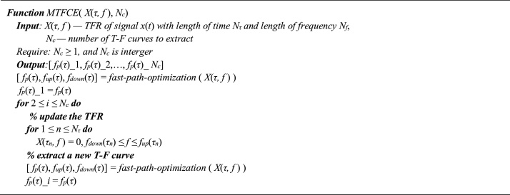
Pseudocode for the MTFCE algorithm is shown in Fig. 1. The Multiple Time-Frequency Curve Extraction (MTFCE) algorithm iteratively applies the fast path-optimization approach to extract multiple curves from the TFR. After a single T-F curve is extracted from the TFR, the TFR is updated by resetting the amplitude of the extracted curve (from the lower boundary to upper boundary) to zero.

Fig. 1.

Pseudocode for the MTFCE algorithm.

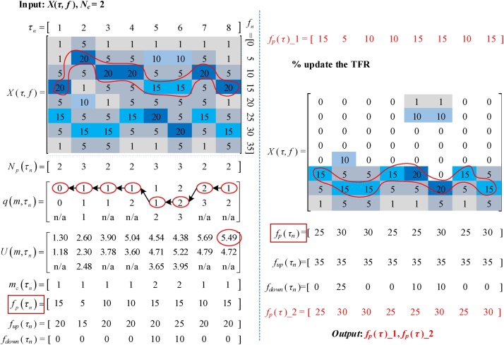
To demonstrate more details about the fast path optimization approach and the MTFCE algorithm, an example of using the MTFCE algorithm to extract two T-F curves from the TFR is shown in Fig. 2

Fig. 2.

Schematic results of multiple curve extraction from TFR.

In this example, the TFR X(τ, f) of a signal x(t) is an 8*8 matrix. It can be observed that there are two T-F curves and the one with lower frequencies is more significant, marked in the TFR on the left side of Fig. 2. First, the peaks at each moment are determined and the number of peaks at each moment N_p(τ_n) is obtained. Then, q(m, τ_n) and U(m, τ_n) are calculated from τ₁ to τ₈ as given in Fig. 2. The peak at τ₈ which has the maximum value of U(m, τ_n) is taken as the end point of the T-F curve. Therefore, the first peak at τ₈ is considered as the end point. Then, the whole T-F curve can be extracted by tracking the peaks backward based on the result of q(m, τ_n). From the track, m_c(τ_n) is determined which mth peak should be extracted for each moment. Then, f_p(τ_n) is obtained correspondingly. The upper boundary f_up(τ_n) and lower boundary f_down(τ_n) are also determined. Thus, the first T-F curve f_p(τ)_1 is extracted. Also, even though the peaks at τ₅ and τ₆ do not have the maximum amplitude curve, f_p(τ)_1 is successfully extracted. It shows that the fast path optimization approach can prevent frequency jumps. To further extract the second T-F curve, the TFR X(τ, f) is updated, shown on the right side of Fig. 2, by setting the amplitude of the TFR within the lower boundary the upper boundary to zero at each moment. Again, applying the fast path optimization approach to the updated TFR, then the second T-F curve is extracted as f_p(τ)_2. It can be seen that the results of f_p(τ)_1 and f_p(τ)_2 agree with the corresponding frequencies of the T-F curve marked in the original TFR and the updated TFR, respectively.

The Matlab function for the fast path optimization ecurve.m [21] and the function for the MTFCE algorithm mltcurve.m are included in the. zip file.

Automatic Bearing fault diagnosis under time-varying speed conditions via MTFCE algorithm

Vibration signal analysis is an important technique for bearing fault diagnosis. Transforming the vibration signal of a bearing into the frequency domain, bearing faults can be identified since each type of fault has a specific Fault Characteristic Frequency (FCF) which is proportional to the Shaft Rotational Frequency (SRF). The Fault Characteristic Coefficient (FCC), i.e. the ratio of the FCF to the SRF, can be determined by the bearing structural parameters. The FCC of the outer race fault (FCC_o) and the FCC of the inner race fault (FCC_I) can be calculated as follows [1]:

$$FC{C}_o=\frac{n_b}{2}\left(1-\frac{d}{D}\cos \varphi \right)$$

$$FC{C}_I=\frac{n_b}{2}\left(1+\frac{d}{D}\cos \varphi \right)$$

where n_b is the number of rolling elements, d is the diameter of the rolling element, D is the pitch diameter of the bearing, Φ is the angle of the load from the radial plane. Bearing faults can be diagnosed by observing the FCF in the frequency spectrum of the vibration signal if the bearing is under constant rotational speed. However, bearings often operate under time-varying speed conditions which make the FCF also time-varying. Therefore, bearing faults cannot be simply observed in the frequency domain.

Time-frequency analysis can be used to analyze a signal in time-frequency domain which renders it an effective technique for bearing fault diagnosis under time-varying speed conditions even without measuring the rotational speed. With the time-frequency analysis techniques, for instance, the STFT and wavelet transform, the TFR of the signal can be obtained to reveal the time-frequency characteristics of a signal. The Instantaneous Fault Characteristic Frequency (IFCF), its harmonics, and the Instantaneous Shaft Rotational Frequency (ISRF) show as time-frequency curves in the TFR of the vibration signal when the bearing is faulty.

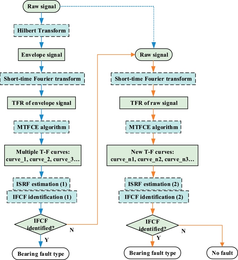
By extracting multiple time-frequency curves from the TFR and identifying the IFCF and the ISRF from the extracted time-frequency curves, bearing faults can be diagnosed under time-varying speed conditions without using a tachometer to measure the rotational speed [16]. The proposed method for automatic bearing fault diagnosis under time-varying speed conditions contains the following steps:

• •Step 1: applying Hilbert transform to the raw signal to obtain the envelope signal;
• •Step 2: applying the STFT to the envelope signal to obtain the TFR of the envelope signal;
• •Step 3: using the Multiple Time-Frequency Curve Extraction (MTFCE) algorithm to extract multiple time-frequency curves from the TFR;
• •Step 4: estimating the ISRF as the T-F curve of the lowest frequency;
• •Step 5: calculating the point-to-point frequency ratios of each curve to the estimated ISRF (i.e. for each curve, the result is a series of frequency ratios), the average of the ratios of each curve and the variance of the ratios of each curve, then, identifying the IFCF by using the tolerant error of average ratio to the FCC of different fault types and the tolerant variance of the ratio;
• •Step 6: diagnosing the fault with the result of IFCF identification.

Considering the fact that the ISRF may not appear in the TFR of the envelope signal, more steps are needed to complete the method.

• •Step 7: applying the STFT to the raw signal to obtain the TFR of raw signal if no IFCF is identified in Step 7;
• •Step 8: using the MTFCE algorithm to extract multiple time-frequency curves from the TFR obtained in Step 8;
• •Step 9: taking the T-F curve of the lowest frequency as the newly estimated ISRF;
• •Step 10: calculating the frequency ratios of each curve obtained in step 2 to the newly estimated ISRF, the average of the ratios of each curve and the variance of the ratios of each curve, then, identifying the IFCF by using the tolerant error of average ratio to the FCC of different fault types and the tolerant variance of the ratio;
• •Step 11: diagnosing the fault with the result in step 11.

A flowchart for the method for automatic bearing fault diagnosis under time-varying speed conditions is shown in Fig. 3. The procedure of the bearing fault diagnosis follows the steps described above. With the exception of the STFT and the MTFCE, the main modules of the bearing fault diagnosis include ISRF estimation and the IFCF identification.

Fig. 3.

Flowchart of bearing fault diagnosis under time-varying speed conditions via multiple time-frequency curve extraction algorithm.

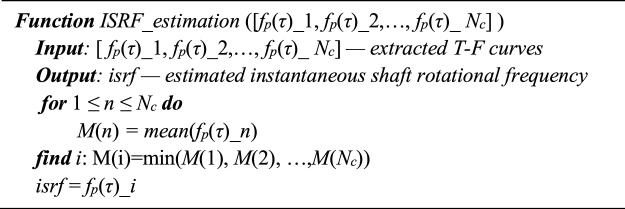
The ISRF is estimated as the time-frequency curve with the lowest frequency among all the extracted time-frequency curves. To determine which time-frequency curve has the lowest frequency, the average frequency of each extracted time-frequency curve is calculated, then the curve of the minimum average frequency is considered as the ISRF. Pseudocode for the ISRF estimation is shown in Fig. 4.

Fig. 4.

Pseudocode for the ISRF estimation.

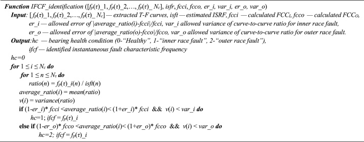
The identification of the IFCF utilizes the FCC since the ratio of the FCF to shaft rotational speed equals the FCC regardless of the variation of the rotational speed. The average point-to-point ratio of two curves is employed to measure the relation of two time-frequency curves. If the IFCF is properly extracted from the TFR, then the average ratio of the IFCF to the estimated ISRF should be approximately the FCC. A parameter defined as the allowed error of |average_ratio-FCC| / FCC is proposed to estimate the error between the calculated curve-to-curve average ratio and the FCC in reality. Additionally, the allowed variance of curve-to-curve ratio is proposed to prevent the case where the IFCF is not properly extracted but the average ratio approximately equals the FCC. Therefore, if the average ratio of a time-frequency curve to the estimated ISRF satisfies the restriction of the allowed error and the allowed variance of curve-to-curve ratio, then the curve is identified as the IFCF. Pseudocode for the IFCF identification is shown in Fig. 5. In this automatic bearing fault diagnosis method, bearing faults cover two types of faults, i.e. inner race fault and outer race fault. For other types of faults, a similar IFCF identification procedure can be added to the method frame if the FCC of the fault is known.

Fig. 5.

Pseudocode for the IFCF identification.

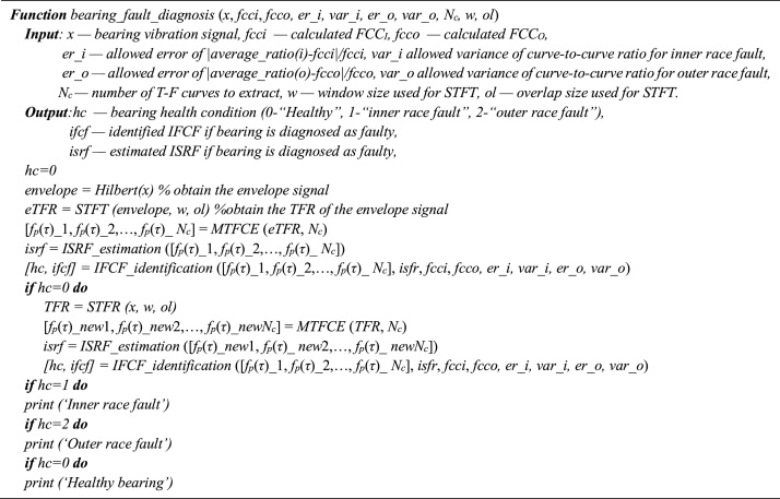
Pseudocode for the automatic bearing fault diagnosis under time-varying speed conditions without measurement of shaft rotational speed is shown in Fig. 6.

Fig. 6.

Pseudocode for automatic bearing fault diagnosis under time-varying speed conditions without measurement of shaft rotational speed.

It can be seen that there are 10 inputs for the automatic bearing fault diagnosis method. Among them, FCCI and FCCO are determined by the bearing structure parameters, and x is the bearing vibration signal. Therefore, there are 7 method-related parameters, including er_i, var_i, er_o, var_o, N_c, w, and ol that need to be selected by the user. Parameters er_i, var_i, er_o, and var_o are used as restrictions for the IFCF identification. If the value is set too small, the T-F curve extracted from the signal of a faulty bearing may not be identified as the IFCF. On the contrary, if the value is set too large, the extracted T-F curve may be identified as the IFCF by mistake. As to the number of the extracted T-F curves N_c, the selection is a trade-off between the accuracy and computational cost. It should be selected as large enough to extract the IFCF or the ISRF at an acceptable computational cost. Additionally, w and ol are the parameters for the STFT. A larges window size w can provide a better frequency resolution in the frequency domain, however, requires a higher computational cost. For the overlap size ol, a larger ol can provide a better time resolution in the time domain, however, requires a higher computational cost. The quality of the TFR impacts on the result of the T-F curve extraction, therefore, w and ol should be well tuned to ensure the accuracy of the fault diagnosis. Overall, users need to tune the 7 method related parameters when using the proposed method.

The Matlab function for the ISRF estimation ISRF_estimation.m, the function for the IFCF identification fault_diagnosis.m, and the function for the automatic bearing fault diagnosis bearing_fault_diagnosis.m are attached in the. zip file. Additionally, an application example main_bearing_fault_diagnosis_example.m which utilizes the proposed method is also attached in the. zip file. For the Hilbert transform, Hilbert() is used to obtain the envelope signal. For the STFT, spectrogram() is employed to obtain the TFR of a signal.

Method validation

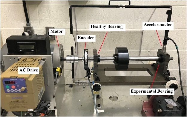
Vibration signals of bearing with different health conditions measured under time-varying rotational speed conditions are used to validate the method. Signals can be found in [19]. Experiments are performed on a SpectraQuest machinery fault simulator (MFS-PK5M). The experimental set-up is shown in Fig. 7. A motor drives the shaft and an AC drive is used to adjust the rotational speed. The shaft is supported by two ER16 K ball bearings, the left one is a healthy bearing and the right one is the experimental bearing, replaced by bearings of different health conditions. Structural parameters of the bearings are given in Table 1. An accelerometer (ICP accelerometer, Model 623C01) is placed on the housing of the experimental bearing to collect the vibration data. Additionally, an incremental encoder (EPC model 775 with CPM = 1024) is installed to measure the shaft rotational speed.

Fig. 7.

Experimental set-up [19].

Table 1.

Parameters of bearings.

Bearing type	Pitch diameter	Ball diameter	Number of balls	FCCI	FCCO
ER16K	38.52 mm	7.94 mm	9	5.43	3.57

The proposed method is examined by all the 36 datasets provided in [19]. However, for brevity, only selected results are shown here. The selected results are obtained by applying the proposed method to three signals measured from bearings with different health conditions, one measured from a bearing with inner race fault, one from a bearing with outer race fault, and the other one from a healthy bearing.

According to the information provided in [19], signals are all collected at 200 kHz for 10 s. Also, FCC_I = 5.43 and FCC_O = 3.57. Since the sampling frequency is too high which leads to very high computational cost, the signal is down-sampled 10 times to fix the computation. If high computational cost is not a concern, then it is not necessary to down-sample the signal.

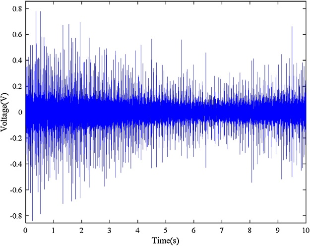
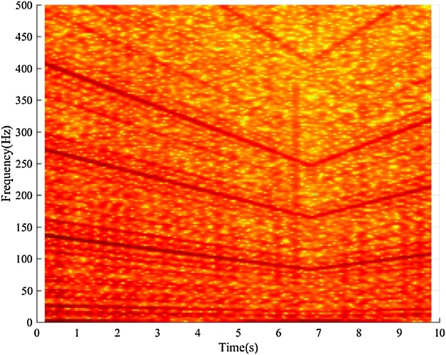
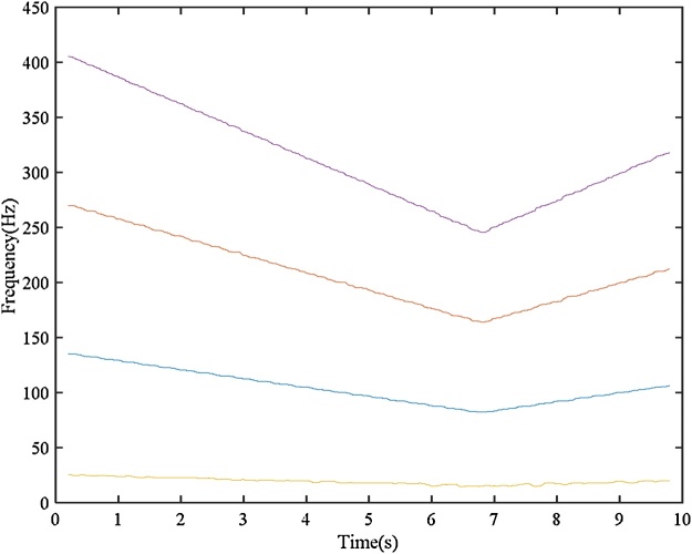
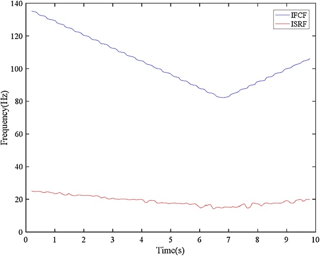
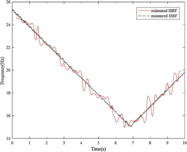
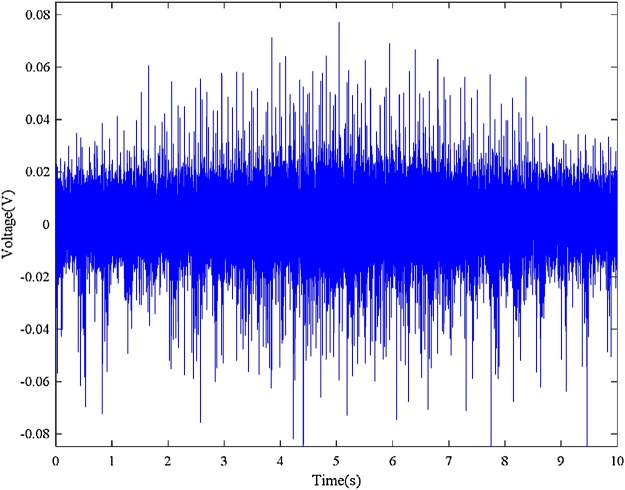
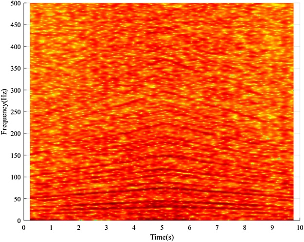
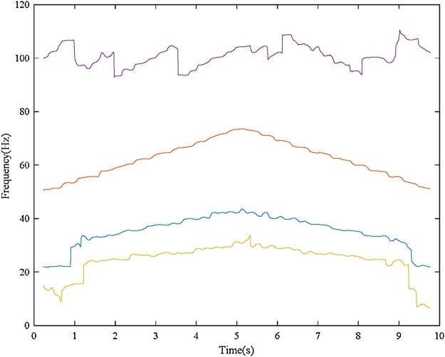
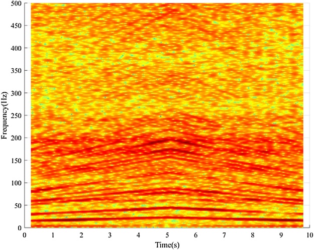
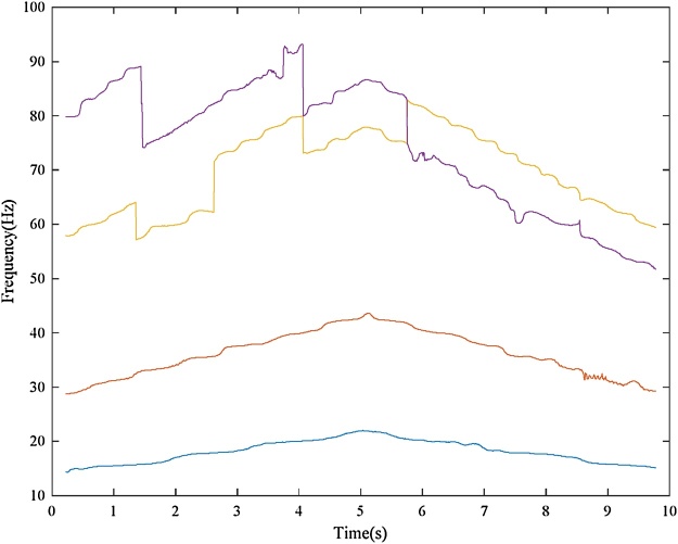
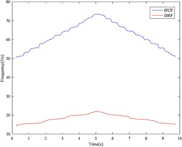
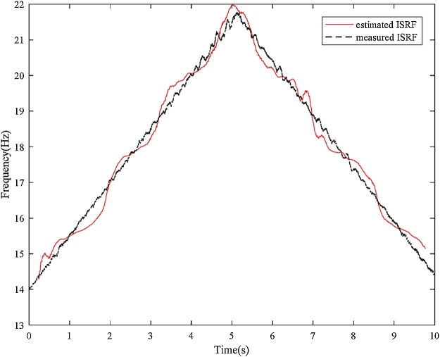
• 1Bearing with inner race fault Input: bearing vibration signal x(t) = I-D-2.mat (Channel_1) [19], fs = 200,000 Hz, FCC_I= 5.43 and FCC_O= 3.57, N_c = 4, er_i=0.02, var_i = 0.11, er_o = 0.055, var_o = 0.09, w = 9000, and ol = 8800. Additionally, Shaft encoder signal s(t) = I-D-2.mat (Channel_2).Results: “Inner race fault”. The down-sampled bearing vibration signal is shown in Fig. 8. The obtained TFR of the envelope signal via the Hilbert transform and STFT is shown in Fig. 9. Then, the T-F curves extracted from the TFR of the envelope signal via the MTFCE are shown in Fig. 10. By estimating the bottom T-F curve as the ISRF, the second lowest T-F curve is identified as the IFCF with the average curve-to-curve ratio = 5.4311 (matching the FCC_I) and the variance of the curve-to-curve ratio = 0.0148. The estimated ISRF and the identified IFCF are shown in Fig. 11. Additionally, the measured ISRF is obtained from the shaft encoder signal. A comparison of the estimated ISRF to the measured ISRF is shown in Fig. 12. The average error |estimated ISRF-measured ISRF| / measured ISRF = 1.84%.
• 2Bearing with outer race fault Input: bearing vibration signal x(t) = O-C-1.mat (Channel_1) [19], fs = 200,000 Hz, FCC_I = 5.43 and FCC_O = 3.57, N_c = 4, er_i = 0.02, var_i = 0.11, er_o = 0.055, var_o = 0.09, w = 9000, and ol = 8800. Additionally, Shaft encoder signal s(t) = O-C-1.mat (Channel_2). Results: “Outer race fault”. The down-sampled bearing vibration signal is shown in Fig. 13. The obtained TFR of the envelope signal via the Hilbert transform and STFT is shown in Fig. 14. Then, the T-F curves extracted from the TFR of the envelope signal via the MTFCE are shown in Fig. 15. By estimating the bottom T-F curve as the ISRF, no IFCF is identified from the extracted curves. Therefore, the TFR of the bearing vibrations signal should be investigated, which is obtained via the STFT, shown in Fig. 16. Then, the T-F curves extracted from Fig. 16 via the MTFCE are shown in Fig. 17. By estimating the bottom T-F curve in Fig. 17 as the new ISRF, the second top T-F curve in Fig. 15 is identified as the IFCF with the average curve-to-curve ratio = 3.4378 (matching the FCC_O) and the variance of the curve-to-curve ratio = 0.0038. The estimated ISRF and the identified IFCF are shown in Fig. 18. Additionally, the measured ISRF is obtained from the shaft encoder signal. A comparison of the estimated ISRF to the measured ISRF is shown in Fig. 19. The average error |estimated ISRF-measured ISRF| / measured ISRF = 1.44%.
• 3Healthy bearing Input: bearing vibration signal x(t) = H-D-3.mat (Channel_1) [19], fs = 200,000 Hz, FCC_I = 5.43 and FCC_O = 3.57, N_c = 4, er_i = 0.02, var_i = 0.11, er_o = 0.055, var_o = 0.09, w = 9000, and ol = 8800. Additionally, Shaft encoder signal s(t) = H-D-3.mat (Channel_2). Results: “Healthy bearing”. The down-sampled bearing vibration signal is shown in Fig. 20. The obtained TFR of the envelope signal via the Hilbert transform and STFT is shown in Fig. 21. Then, the T-F curves extracted from the TFR of the envelope signal via the MTFCE are shown in Fig. 22. By estimating the bottom T-F curve as the ISRF, no IFCF is identified from the extracted curves. Therefore, the TFR of the bearing vibrations signal is further investigated, which is obtained via the STFT, shown in Fig. 23. Then, the T-F curves extracted from Fig. 23 via the MTFCE are shown in Fig. 24. By estimating the bottom T-F curve in Fig. 24 as the new ISRF, still no IFCF is identified from Fig. 21. Therefore, the bearing is diagnosed as healthy. It is worth mentioning that, in Fig. 22, the average ratio of the second highest curve to the bottom curve is 3.6323 which matches the FCCo within the allowable relative error er_o. The bearing will be diagnosed as faulty with outer race fault if we were to only use the average ratio for the IFCF identification as in [16]. However, the variance of the curve-to-curve ratio of these two curve is 1.3439 which is above the allowable variance var_o. Therefore, the accuracy of the proposed automatic bearing fault diagnosis method is improved with the proposed approach.

Fig. 8.

Bearing vibration signal (inner race fault).

Fig. 9.

TFR of envelope signal (inner race fault).

Fig. 10.

Extracted T-F curves from the TFR of envelope signal (inner race fault).

Fig. 11.

Estimated ISRF and identified IFCF (inner race fault).

Fig. 12.

Comparison of the estimated ISRF to the measured ISRF (inner race fault).

Fig. 13.

Bearing vibration signal (outer race fault).

Fig. 14.

TFR of envelope signal (outer race fault).

Fig. 15.

Extracted T-F curves from the TFR of envelope signal (outer race fault).

Fig. 16.

TFR of vibration signal (outer race fault).

Fig. 17.

Extracted T-F curves from the TFR of vibration signal (outer race fault).

Fig. 18.

Estimated ISRF and identified IFCF (outer race fault).

Fig. 19.

Comparison of the estimated ISRF to the measured ISRF (outer race fault).

Fig. 20.

Bearing vibration signal (healthy).

Fig. 21.

TFR of envelope signal (healthy).

Fig. 22.

Extracted T-F curves from the TFR of envelope signal (healthy).

Fig. 23.

TFR of the original signal (healthy).

Fig. 24.

Extracted T-F curves from the TFR of the original signal (healthy).

The same settings of the parameters N_c = 4, er_i = 0.02, var_i = 0.11, er_o = 0.055, var_o = 0.09, w = 9000, and ol = 8800 are valid for 26 datasets provided in [19], including I-A-2, I-A-3, I-B-2, I-B-3, I-D-1, I-D-2, I-D-3, O-A-1, O-A-3, O-B-3, O-C-1, O-C-2, O-D-1, O-D-3, H-A-1, H-A-2, H-A-3, H-B-1, H-B-2, H-B-3, H-C-1, H-C-2, H-C-3, H-D-1, H-D-2, and H-D-3. Since the results are dependent on the obtained TFR, modification of w and ol can lead to different result. By setting w = 9000 and ol = 8000, the results of datasets I-C-3, O-A-2, and O-D-2 are satisfying. By setting w = 7000 and ol = 6800, the results of datasets I-C-1, and I-C-2 are satisfying. Therefore, the proposed method is found valid for 31 datasets out of the 36 datasets. It is believed that further modifications to the parameter could improve the accuracy rate. Users are encouraged to modify the settings of the parameters according to the characteristics of their signal(s) of interest.

It should be mentioned that the performance of the MTFCE algorithm is related to the quality of the obtained TFR. If the vibration signal is blurred by strong noise or interferences, the time-frequency curves may not be properly extracted from the TFR by the MTFCE algorithm. For such cases, bearing fault feature extraction methods should be applied to remove the noise or interference before obtaining the TFR of the signal.

Conclusions

In this paper, the Matlab code for Multiple Time-Frequency Curve Extraction algorithm is given. The MTFCE code can then be used for automatic bearing fault diagnosis under time-varying speed conditions without measuring the speed. Additionally, a new parameter, the allowable variance of the curve-to-curve ratio, is added to the automatic bearing fault diagnosis method aiming to improve the accuracy. Custom Matlab codes are provided in the attached. zip file to enable the method to be applied. Vibration data of bearing with different health conditions measured under time-varying rotational speed conditions are used to demonstrate the approach. The results show that the code and methodology can effectively diagnose the bearing faults under time-varying speed conditions.

Appendix A. Supplementary data

The following are Supplementary data to this article:

References

- 1.Randall R.B., Antoni J. Rolling element bearing diagnostics-a tutorial. Mech. Syst. Signal Process. 2011;25(2):485–520. [Google Scholar]
- 2.Liang M., Soltani Bozchalooi I. An energy operator approach to joint application of amplitude and frequency-demodulations for bearing fault detection. Mech. Syst. Signal Process. 2010;24(5):1473–1494. [Google Scholar]
- 3.Huang H., Baddour N., Liang M. Auto-OBSD: automatic parameter selection for reliable oscillatory behavior-based signal decomposition with an application to bearing fault signature extraction. Mech. Syst. Signal Process. 2017;86:237–259. [Google Scholar]
- 4.He Q., Wu E., Pan Y. Multi-scale stochastic resonance spectrogram for fault diagnosis of rolling element bearings. J. Sound Vib. 2018;420:174–184. [Google Scholar]
- 5.Zhang S., He Q., Ouyang K., Xiong W. Multi-bearing weak defect detection for wayside acoustic diagnosis based on a time-varying spatial filtering rearrangement. Mech. Syst. Signal Process. 2018;100:224–241. [Google Scholar]
- 6.Zhang S., He Q., Zhang H., Ouyang K. Doppler correction using short-time MUSIC and angle interpolation resampling for wayside. IEEE Trans. Instrum. Meas. 2017;66(4):671–680. [Google Scholar]
- 7.Lu S., He Q., Yuan T., Kong F. Online fault diagnosis of motor bearing via stochastic-resonance-based adaptive filter in an embedded system. IEEE Trans. Syst. Man Cybern. Syst. 2017;47(7):1111–1122. [Google Scholar]
- 8.Ding X., He Q. Time – frequency manifold sparse reconstruction: a novel method for bearing fault feature extraction. Mech. Syst. Signal Process. 2016;80:392–413. [Google Scholar]
- 9.Wang T., Liang M., Li J., Cheng W. Rolling element bearing fault diagnosis via fault characteristic order (FCO) analysis. Mech. Syst. Signal Process. 2014;45(1):139–153. [Google Scholar]
- 10.Shi J., Shen C., Jiang X., Huang W., Zhu Z. 2017. An Auto Instantaneous Frequency Order Extraction Method for Bearing Fault Diagnosis under Time-Varying Speed Operation; pp. 2–6. [Google Scholar]
- 11.Algorithm S.S., Resample A., Ye M., Huang J. 2018 XIII Int. Conf. Electr. Mach. 2018. Bearing fault diagnosis under time-varying speed and load conditions via; pp. 1775–1781. [Google Scholar]
- 12.Networks C.N., Algorithm D.L. 2017. Bearing Fault Diagnosis under Variable Speed Using Convolutional Neural Networks and the Stochastic Diagonal Levenberg-Marquardt Algorithm. [DOI] [PMC free article] [PubMed] [Google Scholar]
- 13.Khan S.A., Kim J. Automated bearing fault diagnosis using 2D analysis of vibration acceleration signals under variable speed conditions. Shock Vib. 2016;2016 [Google Scholar]
- 14.Shi J., Liang M., Guan Y. Bearing fault diagnosis under variable rotational speed via the joint application of windowed fractal dimension transform and generalized demodulation: a method free from prefiltering and resampling. Mech. Syst. Signal Process. 2016;68–69:15–33. [Google Scholar]
- 15.Cocconcelli M., Zimroz R., Rubini R., Bartelmus W. STFT based approach for ball bearing fault detection in a varying speed motor. Cond. Monit. Mach. Non-Stationary Oper. 2012:41–50. [Google Scholar]
- 16.Huang H., Baddour N., Liang M. Bearing fault diagnosis under unknown time-varying rotational speed conditions via multiple time-frequency curve extraction. J. Sound Vib. 2018;414 doi: 10.1016/j.mex.2019.05.020. [DOI] [PMC free article] [PubMed] [Google Scholar]
- 17.Huang H., Baddour N., Liang M. Algorithm for multiple time-frequency curve extraction from time-frequency representation of vibration signals for bearing fault diagnosis under time-varying speed conditions. Proceedings of the ASME Design Engineering Technical Conference. 2017;8 [Google Scholar]
- 18.Huang H., Baddour N., Liang M. A method for tachometer-free and resampling-free bearing fault diagnostics under time-varying speed conditions. Measurement. 2019;134:101–117. [Google Scholar]
- 19.Huang H., Baddour N. Bearing vibration data collected under time-varying rotational speed conditions. Data Brief. 2018;21:1745–1749. doi: 10.1016/j.dib.2018.11.019. [DOI] [PMC free article] [PubMed] [Google Scholar]
- 20.Feng Z., Liang M., Chu F. Recent advances in time-frequency analysis methods for machinery fault diagnosis: a review with application examples. Mech. Syst. Signal Process. 2013;38(1):165–205. [Google Scholar]
- 21.Iatsenko D., Mcclintock P.V.E., Stefanovska A. Extraction of instantaneous frequencies from ridges in time – frequency representations of signals. Signal Process. 2016;125:290–303. [Google Scholar]
Associated Data
This section collects any data citations, data availability statements, or supplementary materials included in this article.