Deep Learning in Image Cytometry: A Review

Abstract

Artificial intelligence, deep convolutional neural networks, and deep learning are all niche terms that are increasingly appearing in scientific presentations as well as in the general media. In this review, we focus on deep learning and how it is applied to microscopy image data of cells and tissue samples. Starting with an analogy to neuroscience, we aim to give the reader an overview of the key concepts of neural networks, and an understanding of how deep learning differs from more classical approaches for extracting information from image data. We aim to increase the understanding of these methods, while highlighting considerations regarding input data requirements, computational resources, challenges, and limitations. We do not provide a full manual for applying these methods to your own data, but rather review previously published articles on deep learning in image cytometry, and guide the readers toward further reading on specific networks and methods, including new methods not yet applied to cytometry data. © 2018 The Authors. Cytometry Part A published by Wiley Periodicals, Inc. on behalf of International Society for Advancement of Cytometry.

Automation of microscopy, including sample handling and microscope control, enables rapid collection of digital image data from cell samples, tissue slides, and cell cultures grown in multi‐well plates, transforming imaging cytometry into one of the most data‐rich scientific disciplines. The first approaches to automated analysis of microscopy data appeared already in the 1950s, and a wealth of methods for finding cells and subcellular regions, and designing features that describe phenotypic variations in response to disease or potential drugs, have been developed over the years 1, 2. These approaches, often combined with conventional machine learning methods, have been successfully used for many complex biological datasets 3, 4. However, task‐specific algorithm optimization and feature engineering is a challenging and time‐consuming task, and often insufficient for dealing with global and local contextual variations.

Thanks to increased computing power and large amounts of annotated images of natural scenes, methods based on the ideas about neural network and deep learning, that have been around for a long time, are finally working in practice and we now see the fast emergence of approaches to image analysis where the computer learns the task at hand from examples and automatically exploits the input images for measurements or decisions. A comparison between conventional and deep learning workflows is illustrated in Figure 1.

Figure 1.

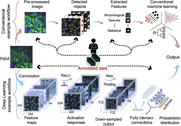
Overview of conventional versus deep learning workflows. The human in the center provides input in the form of, for example, parameter tuning and feature engineering in each step of the conventional workflow (black dashed arrows) using annotated data. Conversely, the deep learning workflow requires only annotated data to optimize features automatically. Annotated data is a key component of supervised deep learning as illustrated in the example classification workflow. Other example tasks, as discussed in the text, follow a similar pattern. The example image was provided by the Broad bioimage benchmark collection.

Deep learning relates to fundamental concepts in neuroscience. A neuron is an electrically excitable cell that receives signals from other neurons, processes the received information, and transmits electrochemical signals to other neurons 5. The input signal to a given neuron needs to exceed a certain threshold for the neuron to be activated and further transmit a signal. The neurons are interconnected and form a network that collectively steers brain mechanisms 6.

Inspired by our brain, an artificial neural network is an abstracted interconnected network, consisting of neurons (perceptrons) grouped into layers. It consists of an input layer aggregating the input signals from other connected neurons, one or many hidden layers of thresholds or weights, and an output layer for predictions. Each neuron takes the input from the neurons of the previous layer using various weights (determined by training) and computes an activation function (e.g., sigmoid function) to stimulate a non‐linear behavior, which is relayed onto the next layer of neurons. A deep neural network (DNN) is formed by cascading several such neurons in multiple layers to form a richer hierarchical network commonly known as a multilayer perceptron (MLP), where all neurons in the previous layer are densely (or fully) connected to the neurons of succeeding layers 7, 8, 9, 10. The neurons within the layers may also be connected to themselves to enable the solving of more complex problems. However, they are restricted to input data structured in vector form, which limits their suitability to images. To overcome this, convolutional neural networks (CNNs) were developed 11, wherein 2D filters (or convolutional kernels) are used to process local image information in matrix form.

From a biological perspective, a CNN approximately emulates the primate brain's visual system 12, 13, 14, which employs a combination of convolutional and pooling layers (see section on “Overview of Key Concepts” below) before the dense layers to progressively encode richer representations in an image 15. Filter weights in “deep” CNNs are updated iteratively using annotated image examples. Hereafter we often refer to such methods as “deep learning” for brevity, though deep learning as such is a broader concept than CNNs. Deep learning has several advantages over conventional methods. For instance, these techniques directly learn discriminative representations (or features) from image examples, and effectively leverage the feature interaction and hierarchy within the data, resulting in a simplified feature‐extraction and selection process. Additionally, the performance of a system based on deep learning can be improved systematically by training iteratively on a larger number and variety of examples. Furthermore, a pre‐trained model (i.e., a trained network) from one domain can be adapted through “fine‐tuning” and applied to the same task in a new domain, given that underlying data distributions of both tasks are similar enough. This contrasts to most other learning approaches where the model needs to be completely re‐trained when new observations are made available.

On the down‐side, training a deep neural network from scratch requires massive amounts of annotated data, or data that in some way represent the desired output. Furthermore, the network architecture is often complex, making it difficult to interpret the link between the input data and the predictions.

Excellent previous reviews of the broader concepts of deep learning have been presented for medical image analysis 16, 17, health informatics 18, and microscopy 19. The focus of this review is to highlight how deep learning is currently used for image cytometry, including cytology, histopathology, and high‐content image‐based screening for drug development and discovery. We aim to describe this very quickly emerging branch of image cytometry and explain how it differs from previous “classical” approaches to detect objects, extract features, and/or classify morphological changes, and treatment responses at the microscopic level.

We start by defining the key concepts, terms, and vocabulary used in deep learning. We thereafter review the application areas of deep learning in image cytometry, and highlight a series of successful contributions to the field. Then, we discuss challenges and limitations that are often encountered when applying deep learning in image cytometry. Finally, we discuss some of the most recent method developments and highlight novel techniques that have not yet been used for cell analysis in microscopy data, but have the potential to advance the field in the future. As a guide to further reading this review includes a table with a short summary and links to 256 articles on deep learning in cytometry published prior to August 31, 2018, categorized based on imaging modality, task, and biological sample type.

Overview of Key Concepts

Deep learning architectures come in many flavors, and before going further into the descriptions of deep learning methods, we explain some key concepts:

Convolution

A convolution can be equivalent to applying a filter kernel to an image, such as a 3×3 mean filter with weight values set to one. To determine the output pixel values, a mean filter slides over the input image. For each pixel position, the kernel weights are multiplied by the pixel values in the corresponding region covered by the kernel, then summed together and divided by the kernel size. In other words, a convolution is a specialized type of linear operation that performs two functions: multiplication and addition. To encode the representations (as illustrated in Fig. 2), an element‐wise product between the weights of the kernel and the receptive field of the input image data is calculated at each location and summed to determine the value in the corresponding position of the feature map (or output image).

Figure 2.

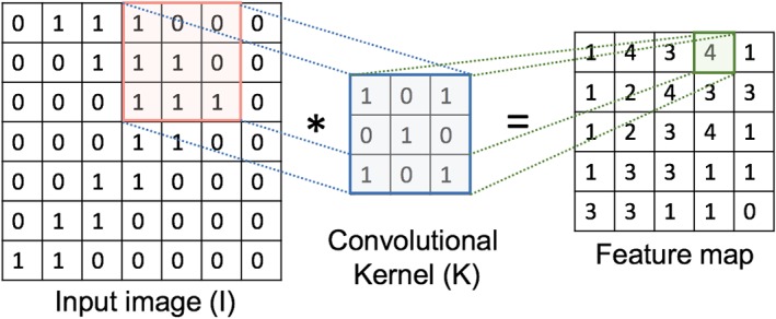
An example of an input image Ι_7x7 convolved with a filter k_3x3 with weights of zeros and ones to encode a representation (feature map). The receptive field is highlighted in pink and the corresponding output value for the position is marked in green. [Color figure can be viewed at wileyonlinelibrary.com]

Receptive Field

The receptive field (RF) is the extent of the convolution operation where local information (i.e., neighboring pixels) in an image sub‐region is taken into account. Locally it is simply the filter size, but in a layered downsampling network it could also mean the region in the input image from which information is propagated.

Activation Function

An activation function is an operation to threshold the calculated output of a convolution prior to submitting the signal to the next layer of the network. The choice of activation functions has a significant implication on the training process and network performance. Their usage depends on the type of network and also on the type of layer in which they operate. Non‐linear operations, such as sigmoid or hyperbolic tangent (tanh) functions, were previously common, but the rectified linear unit (ReLU, 20) is currently the mainstream activation function since it accelerates the convergence of gradient‐based learning and circumvents the problem of vanishing gradients (discussed below). Softmax 21 activation is usually employed in the final layer of a CNN‐based classifier, where its output is equivalent to a categorical probability distribution that determines the class of each input image (or pixel).

Feature Maps

The feature map is the resulting output of the convolution and activation function operations. The dimensions of the resulting feature maps are controlled by three user‐defined parameters (often referred to as hyper‐parameters): depth, stride, and zero‐padding. These hyper‐parameters are specified before performing any convolution operations. The depth here corresponds to the number of convolution kernels (depth is sometimes also used for the total number of layers in the network). The stride is the number of pixels by which the kernel shifts over the input image in each step and determines the overlap between individual output pixels. Zero padding is used to circumvent the reduction in output image size produced by convolution operations (by padding the input image with zeros at the borders).

Pooling

Pooling is an operation to down‐sample the output of the convolutions, similar to binning. The most common pooling operation is max pooling, which outputs the maximum value in a local neighborhood of each feature map (as illustrated in Fig. 3), and discards all the other values. It progressively reduces the spatial dimensions of the given feature maps, and thus decreases the number of pixels to process in the next layers of the network, while maintaining information important for the task at hand 8. There are several other pooling operations such as L2‐norm pooling and global average pooling 22. Pooling reduces the complexity of the previously encoded representations, and can thus be seen as a regularization technique that combats the problem of overfitting (see below).

Figure 3.

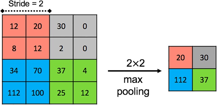
The sub‐sampled output of a max‐pooling operation with a stride of 2 applied on an input image (I). [Color figure can be viewed at wileyonlinelibrary.com]

Densely (or Fully) Connected Layer

In a densely or fully connected layer each neuron of the input layer is connected to every neuron in the succeeding layer, as illustrated in Figure 4a. This combines all representations encoded from the previous layers. For 2D feature maps this is done by flattening the maps into a vector, followed by vector–matrix multiplication. In contrast to the local connection style of convolutional layers, a fully connected layer follows the same connectivity as an MLP. Depending on the complexity of the task, a single or a series of fully connected layers are often added prior to the final classification output layer.

Figure 4.

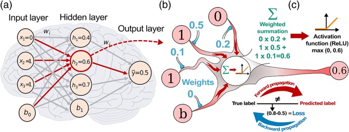
Learning process of a DNN. (a) A dense layer with an input layer where all the encoded representations from the previous layers are fully connected to the next layers. (b) Zoomed‐in view of an example neuron showing the forward propagation to compute the output ȳ, where the non‐negative activations are defined using the ReLU. (c) Gradient‐decent based optimization of the loss function in a forward/backward propagation. [Color figure can be viewed at wileyonlinelibrary.com]

Learning and Optimization

A process to determine the set of optimal values of trainable parameters (e.g., kernel weights in convolution layers and weights in dense layers), as shown in Figure 4b. These parameters are optimized by minimizing a loss function, such as cross‐entropy loss; thus diminishing the discrepancies between the predicted outputs and the given annotations. On a training dataset, the network performance under a particular set of parameters is computed iteratively by a loss function through forward propagation, followed by backpropagation. Backpropagation propagates the loss backward from the output to input layers for computing the gradients of each parameter with respect to the loss. The parameters are then updated using gradient descent optimizers 22. The gradient is a measure of how much the loss changes with respect to changes in parameter values. This iterative process requires many steps, and is the main reason why training a deep neural network requires substantial computational power and time. Although neuroscientists have long rejected the idea that learning through backpropagation is occurring in the human cortex, intriguing possible mechanisms refuting this rejection have been recently suggested 23, 24.

Overfitting and Underfitting

Overfitting occurs when the parameters of a model fit too closely to the input training data, without capturing the underlying distribution, and thus reducing the model's ability to generalize to other datasets. Conversely, underfitting is the result of an excessively simple model which is unable to capture the underlying distributions of the input data. Both overfitting and underfitting lead to poor predictions on unseen data. Regularization techniques, as described below, strive to balance over‐ and underfitting, and enable the model to both adequately fit the training data and generalize well to new data.

Dropout

A regularization technique that reduces the interdependent learning among the neurons to prevent overfitting. Some neurons are randomly “dropped,” or disconnected from other neurons, at every training iteration, removing their influence on the optimization of the other neurons. Dropout creates a sparse network composed of several networks—each trained with a subset of the neurons. This transformation into an ensemble of networks hugely decreases the possibility of overfitting, and can lead to better generalization and increased accuracy 25.

Batch Normalization

A regularization technique that operates between the layers by continuously taking the output of a particular layer and normalizing it before sending it across to the next layer. Batch normalization 26 enables the network to learn faster with better generalized performance. When training with batch normalization, each feature map computed by a convolution operation is normalized separately over each batch of samples.

Skip (Residual) Connections

A skip, or residual connection 27, copies and combines the input of one layer with the output of at least one skipped convolution layer (or block), as illustrated in Figure 5. With an increasing number of layers, the performance of a network may rapidly degrade if the weights become very small during training (referred to as vanishing gradients, 8). Skip connections allow the gradients to flow freely through possibly hundreds of layers, and thus enable the network to learn evenly across all layers.

Figure 5.

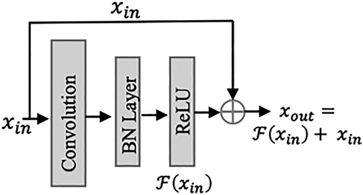
An example of a skip connection, connecting the input with the output of one convolution block (consisting of a convolutional layer, a batch normalization layer, and a ReLU activation function).

Data Augmentation

An approach to overcome the challenges posed by a limited amount of annotated training data. Augmentation is performed by artificially generating more annotated training data, typically by mirroring and rotating the original images (see section on “Data Considerations in Deep Learning” below).

Transfer Learning

This is the concept of employing a pre‐trained network, which was trained on a large number of samples for a similar task, for a new task with little annotated image data. For instance, one can employ transfer learning between imaging modalities by training a network on phase contrast images and using it on fluorescence images 28 for cell segmentation.

Deep Learning Methods

Before delving into how deep learning is used in image cytometry, we briefly describe four general types of deep learning methods.

Convolutional neural networks (CNNs) for segmentation and classification of images are often used in a supervised learning setting, meaning that the networks have to be trained using labeled training samples. The networks are built by stacking many convolutional and pooling layers, as shown in Figure 1. The convolution layers encode the discriminative representations/features, and the pooling layers induce a degree of scale‐ and translation‐ invariance. The earlier layers typically describe local features that have a small receptive field representing a small and local region of the input image, while deeper layers have larger receptive fields, representing information combined from a larger region in the input image 29. All convolution kernels scan across the entire image, meaning that objects need not be at a specific location to be correctly detected 8, 22. Following the final convolution and/or pooling layer the output is flattened and connected to one or more fully connected layers. The neuron(s) in the final output layer give the class probability (either of each input pixel for segmentation or of each input image for classification).

Recurrent neural networks (RNNs) build memory into the network by feedback loops, that is, feeding back the output from a neuron as input to itself. The basic RNN consists of “hidden states” that evolve over time through non‐linear operations on the previous hidden states and the current inputs. Deep RNNs, that attempt to retain information from the distant past, can be difficult to train due to vanishing gradients. Various solutions to this problem have been proposed, such as skip connections across time. Although RNNs are primarily used for one dimensional sequential data they can also be applied to images, whereby they move across space rather than across time, and can potentially capture more long distance interactions than those caught by CNNs 22.

Autoencoders can be used to create a low dimensional representation or “code,” of high dimensional data, much like principal components analysis (PCA), but in a nonlinear manner. An inverse encoder, or “decoder function,” attempts to reconstruct the input from the learned representation 30. Multiple hidden layers can be stacked to the encoder and decoder functions, creating a stacked autoencoder, for learning more complex nonlinear data compression. The learned codes can be made more generalizable using sparsity constraints, which encourage the model to activate fewer neurons 31, or by being trained to “denoise” a noise corrupted version of the input data 32. For image data the fully connected encoder layers are replaced by convolutional and pooling layers, and equivalently the decoder layers by deconvolutional and unpooling layers 33.

Generative adversarial networks (GANs), are networks that can generate synthetic/simulated images that closely mimic the original images 34. In its simplest form a GAN can be thought of as instigating a zero‐sum game between two networks—a generator and a discriminator. The generator creates counterfeit data samples which it hopes to “fool” the discriminator with, while the discriminator attempts to correctly classify the real and fake samples. Convergence is reached when the discriminator can no longer differentiate between real and fake samples. However, convergence is not always guaranteed and GANs currently require careful architectural and hyper‐parameter choices to ensure stability. Generative models can be used to create synthetic datasets, for example, if relatively little annotated data is available 22.

Survey of Published Articles on Deep Learning for Image Cytometry

This review is based on a large number of published articles selected based on automated searches in Scopus, Medline, bioRxiv and arXiv, with the search terms “deep learning,” “convolutional neural networks,” “biomedical images,” “microscopy,” and “cells” (in several different combinations) prior to August 31, 2018. We have also included articles from other application areas in cases where we believe the methodological contributions are of significant interest for the field of image cytometry. We excluded articles where hand‐engineered features were used as the network input, and focus on end‐to‐end representation‐based learning methods where pixel data is the only input. The articles can be grouped into general themes based on tasks (as discussed in the section on “Deep Learning for Image Cytometry”) and based on application areas (as discussed in the section on “Applications of Deep Learning Methods”). Many of the articles are referred to in the following text, but we also provide an overview of the articles in Supporting Information Table S1, and as an infographic in Figure 6. An interactive version including short article summaries is accessible at https://anindgupta.github.io/cyto_review_paper.github.io. The table contains links to each original article, a brief description of key concepts, and a categorization of each article based on tasks (P/S/C): image processing (P), segmentation (S), and classification (C), sample type (T/CL/SB): tissue (T), cells (CL), and subcellular structures (SB), and finally modality (FL/BF/EM): fluorescence (FL), bright field (BF), and electron microscopy (EM). The infographic in Figure 6 serves as a guide to help the reader find articles of interest in relation to a specific task, sample type, or imaging modality, each number in the graphic matching with the corresponding reference. The number of articles in each section can be used to visually assess the current status of the field in terms of popularity and applicability. Given a field of interest, the articles in the corresponding cell of the table become references on the use of deep learning method for this specific task and some of the articles present comparisons of different analysis approaches. It also illustrates the areas of image cytometry where deep learning has been most actively used so far. Note that references to articles not concerned with deep learning for image cytometry are only listed in the regular reference list.

Figure 6.

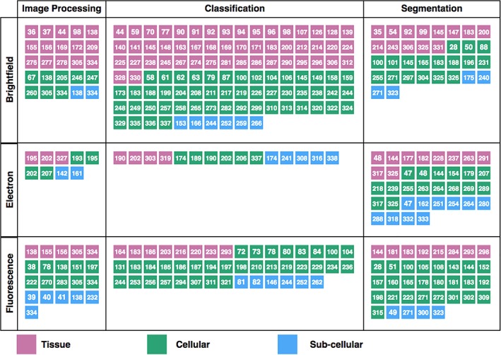
An infographic as a guide to help the readers find articles of interest in relation to a specific task, sample type, or imaging modality, each number in the graphic matching with the corresponding reference. An interactive version linking directly to the source articles can be found at https://anindgupta.github.io/cyto_review_paper.github.io. (138–338) [Color figure can be viewed at wileyonlinelibrary.com]

Deep Learning for Image Cytometry

Deep learning can be used for a number of different data processing and analysis tasks, here grouped into image processing, segmentation, classification, and detection.

Deep Learning for Image Processing

Pre‐processing of microscopy image data is often necessary to compensate for variability in data collection and to improve downstream analysis. For all of these pre‐processing steps both the inputs and outputs are images.

Autoencoders can differentiate between true signal and noise, and Su et al. 35 were among the first to exploit them (using an adaptive dictionary and template) to reduce noise and reconstruct cell nuclei in histopathological images. Later, Rivenson et al., 36 presented an adapted U‐Net architecture (an autoencoder with skip connections, see section on “Deep Learning for Segmentation”) to computationally improve the resolution of bright field images of tissue samples acquired with a 40×/0.95NA objective to be adjusted such as to achieve a resolution that was equivalent to images acquired with a 100×/1.4NA oil immersion objective. Using a similar approach, Rivenson et al. 37 improved the quality of mobile phone microscopy data to match that of high quality bench‐top microscopy (with respect to signal‐to‐noise ratio, stain normalization, aberrations and distortions). Weigert et al. 38 presented a customized U‐Net‐based content aware restoration network, and successfully recovered 3D isotropic resolution in fluorescence microscopy data. Such high‐quality restoration equates to faster imaging times with less phototoxicity; thus enabling the imaging and analysis of more sensitive samples.

Recently, Wang et al. 39 employed GANs to improve the resolution of wide‐field fluorescence microscopy images acquired with a 10×/0.4NA objective and achieved a resolution that is equivalent to images acquired with a 20×/0.75NA objective. They also applied their GANs to diffraction‐limited confocal images and achieved a 2.6× increase in resolution, corresponding to the resolution of stimulated emission depletion microscopy images. Ouyang et al. 40 combined CNNs and GANs to perform fast super‐resolution reconstruction for localization microscopy using a limited number of frames and/or wide‐field microscopy images. Nehme et al. 41 employed a fully convolutional encoder‐decoder network to achieve fast super‐resolution reconstruction in single‐molecule localization microscopy, without requiring any prior knowledge of the structure of interest.

Color and intensity variations in hematoxylin and eosin (H&E) stained tissue samples from different labs, instruments, and imaging sites may influence CNN performance, as reported by Ciompi et al. 42, and stain normalization prior to training may be necessary. Janowczyk et al. 43 employed autoencoders to achieve unsupervised stain normalization using a novel tissue distribution matching technique for color standardization. Another way to account for stain variability is to include stain differences in the training stage—so called stain or color augmentation. Tellez et al. 44 performed stain augmentation directly on H&E channels for whole slide mitosis detection in Breast Histology, and Arvidsson et al. 45 implemented color augmentation in the HSV space to generalize CNNs for prostate cancer classification for multiple imaging sites. Bentaieb et al. 46 performed stain normalization by style transfer across datasets using a GAN coupled to a CNN for end‐to‐end histopathology image classification and tissue segmentation.

Deep Learning for Segmentation

Segmentation, meaning to divide an image to its meaningful parts or objects, requires making accurate local predictions while accounting for global context. One of the first applications of deep learning for segmentation in biomedical image analysis employed a sliding‐window CNN as a pixel classifier to segment neuronal membranes in patches of electron microscopy (EM) images 47. This approach involves a trade‐off, whereby smaller patches sacrifice contextual information for location accuracy and vice versa. To resolve this, Ronneberger et al. 48 presented a more elegant network architecture, referred to as U‐Net, which uses contracting convolving encoder layers (learning global context) skip‐connected to expanding up‐sampling decoder layers (learning high‐resolution location). They also performed random elastic deformations on annotated training data to augment their small training dataset (as described below in the section on “Data Considerations in Deep Learning”). The U‐Net architecture achieved excellent results for three different segmentation tasks: neuronal structures in EM images; Glioblastoma–astrocytoma U373 cells in phase contrast microscopy images; and HeLa cells in differential interference contrast (DIC) microscopy images. Cicek et al. 49 extended U‐Net to volumetric images with 3D U‐Net, which incorporates 3D convolution and pooling operations and is trained using only a small number of annotated 2D slices.

Sadanandan et al. 28, showed that the dimensions of U‐Net could be reduced by combining raw images with images pre‐filtered with task specific hand engineered filters, achieving robust segmentation of Escherichia coli and mouse mammary cells in both phase contrast and fluorescence images. In another article Sadanandan et al. 50 combined CNNs and GANs for segmenting spheroid cell clusters in bright field images. Rather than forcing the GAN to re‐create synthetic images, it was recursively used to improve a set of manually drawn segmentation masks, achieving performance gains over a baseline CNN segmentation architecture. Arbelle et al. 51 presented a GAN‐based architecture, named Rib Cage, for segmenting H1299 cells in fluorescence microscopy images. They employed a multistream discriminator network taking three channels as inputs: gray level channel of fluorescent images; manually segmented channel of fluorescent images using the Ilastik software 52; and a concatenation channel of the former two channels. Training was performed using a limited amount of annotated examples in a weakly supervised manner. Their unique discriminator network leads to improved performance over other tested architectures.

Su et al. 35 achieved improved segmentation performance on both brain tumors and lung cancer cell images using stacked autoencoders. They trained the network using edge enhanced images, centered on cells detected during an initial detection stage, and combined them together with manually annotated cell boundaries. Duggal et al. 53 utilized a form of generative model known as a deep belief network 30 for separating touching or overlapping white blood cell nuclei from leukemia in microscopy images. Recently, Haering et al. 54 presented a cycle‐consistent GAN (Cycle‐GAN) for segmenting epithelial cell tissue in drosophila embryos. Their approach circumvents the need for annotated data by employing two generators, where the second generator translates the output of the first generator back to the input space. Despite the fact that the Cycle‐GAN is trained without annotated data, it still demonstrated comparable results to U‐Net.

Deep Learning for Classification and Detection

DNNs can be used for classifying images, and also to detect and classify objects within the image. Depending on the available labeled training data, the images or objects can be classified into two or more classes. It is important to note that the confidence in such multi‐class predictions may vary depending on the amount of labeled data for each class.

Object detection requires both classification and localization of structures. Localization is usually achieved with bounding boxes around the objects of interest, where the outputs are the spatial coordinates of the object, a minimal width and height of the bounding box, and the respective object class. Object detection can be achieved in various ways: (i) regions of interest can be proposed and classified as object or background; (ii) CNN generated feature maps can be used to find bounding boxes; or (iii) networks can be trained end‐to‐end to simultaneously propose bounding boxes and classify objects. The first approach requires a region proposal step prior to classification 55, as used in the Regional CNN (RCNN) model 56. This model, however, is relatively slow as it needs to generate a number of region proposals per image. For faster performance “faster R‐CNN” 57 was proposed, comprising only two networks; one for classification and one for region detection. Hung et al. 58 used a faster R‐CNN architecture to identify and count malaria infected blood cells in bright field images and achieved results comparable to human annotations.

Ciresan et al. 59 used a CNN for detecting mitotic cells in H&E stained breast cancer histology images. In this work, the small training dataset was augmented using mirroring and rotations. The CNN outputs a probability map, and as a post‐processing step, a smoothing filter suppressed noise before detecting mitotic events. Similarly, Wang et al. 60 presented a CNN for classifying neutrophil cells on H&E histology tissue images to identify active inflammation. They combined the CNN with a Voronoi diagram of clusters to deal with complex cellular context. Input data was augmented by horizontal mirroring and random cropping. Mao et al. 61 presented a CNN to classify circulating tumor cells in phase contrast microscopy images. In an another work, Durant et al. 62 leveraged CNNs to classify erythrocytes into 10 unique classes. They also performed rotation and mirroring augmentations and achieved a high degree of accuracy for measuring erythrocyte morphology profiles. Recently, Fleury et al. 63 presented a light‐weight CNN, MobileNet, to detect and classify blood‐borne pathogen images directly on a smartphone.

An alternative approach to object detection is end‐to‐end training for proposing and classifying bounding boxes. For example, You Only Look Once (YOLO, 64), does this by dividing the input image into a rectangular grid and predicting a confidence score for several bounding boxes in each grid and the class probabilities for objects inside each grid. By multiplying the box scores with the class probabilities, one obtains a value per grid‐cell that is thresholded to give the final bounding box predictions. This approach is comparably fast since it only needs one pass through the network per image. Another related method is the Single Shot MultiBox detector 65 which utilizes small convolutional filters for bounding box predictions and extracts feature maps at different scales for class predictions.

CNNs can also be used for image quality control, discarding poor quality images (e.g., those that are out of focus) prior to further analysis. Work by Yang et al. 66 exploited CNNs on synthetically defocused fluorescence images of DAPI stained nuclei to determine the focus level of image patches. Wei et al. 67 employed a CNN, pre‐trained on ImageNet data, to classify the focus of bright field and phase contrast images in numerous z‐level classes. They used this approach to automatically control focus during time‐lapse microscopy.

Transfer Learning and Domain Adaptation

Domain adaptation and transfer learning are two related deep learning methods for reusing acquired knowledge. In transfer learning, the features learned by a CNN are reused for different tasks in a similar domain 68 whereas in domain adaptation a discriminative model trained in one domain is applied to the same task in a different domain 7, 69. Both approaches are useful when labeled data are lacking, such as in image cytometry, where manual annotations are time consuming to make and require a high level of expertise.

For transfer learning, large annotated datasets, like ImageNet 70, can be used to pre‐train state‐of‐the‐art CNNs such as Resnet 27 and Inception 71. The transferred parameter values—providing good initial values for gradient descent—can be fine‐tuned to fit the target data 72. Alternatively, the pre‐trained parameters in the initial layers can be frozen—capturing generic image representations—while the parameters in the final layers can be fine‐tuned to the current task 73. Relative to training from scratch, transfer learning allows the fitting of deeper networks, using fewer task‐specific annotated images, for improved classification performance and generalizability.

The reuse of “off‐the‐shelf” features in domain adaptation was exemplified by Chacon et al. 74 who combined two U‐NET architectures for segmenting mitochondria and synapse EM images. In their case sufficient labeled data was available for one brain region (source domain) but not for another (target domain). However, neural network performance may also degrade under domain adaptation 75. CNNs trained on biomedical images, captured under specific experimental conditions and imaging setups, may have poor generalizability as a consequence of variability in the acquisition and staining processes. This is typical for histology applications. Unsupervised domain adaptation 76 has the potential to resolve this problem. For instance, Yu et al. 77, successfully employed unsupervised domain adaptation for a pre‐trained CNN classifying epithelium‐stroma in H&E images from three independent datasets.

Applications of Deep Learning Methods

In this section we highlight a number of examples where deep learning has been used in image cytometry (broadly defined as extracting measurements from microscopy images of cells or subcellular structures).

Deep Learning for High‐Content Screening

In high‐content screening (HCS), cells are systematically exposed to different perturbants (typically small molecules or siRNA) with the hypothesis that the perturbations of interest induce quantifiable changes in cell morphology. Cells are often labeled with one or more fluorescent stains (such as fluorescence‐labeled antibodies) specifically binding to subcellular components, and imaged by fluorescence microscopy. Imaging flow cytometry (IFC) combines fluorescence microscopy and the high‐throughput capabilities of flow cytometry, simplifying data processing as single cells are imaged, however at the cost of limited spatial information. HCS and IFC both generate large amounts of image data from multiple spatially correlated fluorescence channels, making deep learning a suitable analysis approach 78, 79.

In HCS, Dürr et al. 80 successfully used CNNs for phenotypic classification of cells treated with different biochemical compounds. CNNs have also shown good performance for classifying the subcellular localization of proteins in yeast cells 81, 82. Sommer et al. 83 took an alternative approach for phenotype classification by employing an autoencoder trained on negative control samples (as a self‐learned feature extractor). The features extracted from cells exposed to stimuli were then clustered to obtain groups of stimuli resulting in similar abnormal phenotypes. CNNs have also shown potential in mechanism of action classification directly from raw image data 82. Kensert et al. 72 and Pawlowski et al. 73 grouped chemical compounds by applying networks pre‐trained on ImageNet to the raw images, without any cell segmentation.

Using data from IFC, Eulenberg et al. 78 trained a CNN to classify cells into different stages of the cell cycle. They thereafter extracted the activations in the last layer of the network, and with non‐linear dimensionality reduction reconstructed the correct temporal progression of the full cell cycle. Young et al. 84 developed a real‐time CNN‐based method to count and identify cells in high‐throughput microscopy‐based label‐free IFC. However, deep learning in IFC is still mostly uncharted territory, and the expectations are high that CNNs will reduce manual tuning, subjective interpretation, and variation in the analysis of this data 79.

Deep Learning for Cytology and Histopathology

Cytology and histology are two different approaches for collecting and analyzing samples for diagnostic purposes. In cytology, individual cells are removed from their tissue context, for instance in the form of smears (e.g., cervical or oral). In histology cells are collected either by a needle biopsy or as a section from a larger tissue sample, such as a tumor removed from a patient, with preserved contextual tissue‐level information. Both fields rely on similar microscopy modalities at similar spatial resolutions. Increased adoption of digital whole slide imaging (WSI), especially in histopathology 85, but also in cytopathology 86, has provided a wealth of high‐throughput data that can potentially be analyzed with deep learning. With respect to cervical cancer screening, Zhang et al. 87 used a CNN based on transfer learning that took nuclei centered image patches as input and achieved high classification accuracy for both pap‐smears and liquid‐based cytology images. An important aspect in automated screening systems is accurate segmentation of overlapping cells. Song et al. 88 proposed a multi‐scale CNN to perform an initial segmentation followed by border refinement to account for overlapping cells.

In cytology, it is typically sufficient to have receptive fields large enough to cover individual cells due to the lack of contextual information. In contrast, in order to capture the tissue context in a histopathological analysis, one often needs to consider much larger parts of the sample. This difference, in terms of scale, is a major technical challenge. The processing of a WSI, typically containing several gigapixels of data, is often constrained by limited computer memory. Moreover, scanning hundreds or even thousands of WSIs (typically required for training deep networks) is usually infeasible. On the other hand, a single WSI can contain millions of cells, and in terms of pixels even moderately sized WSI datasets contain an order of magnitude more data than the ImageNet dataset 70. To leverage these properties and to allow efficient processing, most proposed systems rely on patch‐based approaches, where a slide is divided into smaller patches, or tiles 89, 90, 91, 92. Each tile then constitutes a training sample, and thousands of tiles can be extracted from a single WSI. Computational efficiency can be improved further by sampling only potentially relevant regions for further analysis 90, 93. The importance of scale is also reflected in the presence of information at various hierarchical levels within a WSI ‐ cells in a tissue section are not independent, but are components of structures such as glands, and these higher level structures are in many cases crucial for histopathological diagnostics. Stacked networks, and other types of multi‐resolution approaches, are applied to address this issue 94, 95, 96.

The interest in applying image analysis to histopathology has recently manifested in the organization of several challenges, such as the detection of metastatic breast cancer from lymph node biopsies in CAMELYON 89, 97, mitosis counting in TUPAC16 92, HER2 biomarker scoring 98, and segmentation of colon glands in GlaS 99. All of these challenges have been dominated by solutions relying on deep learning.

Deep Learning for Time‐Lapse Image Analysis

Time‐lapse imaging holds great promise for elucidating the complex behavior of cells over time (such as proliferation, division, differentiation, and migration). To fully utilize this data, however, it is necessary to both detect and track cells. Akram et al. 100 presented a joint detection and tracking framework where first a cell proposal CNN was used to localize cells, followed by a graphical model for connecting cell proposals between adjacent frames. They used this approach for HeLa and GOWT1 fluorescence cell images, as well as glioblastoma–astrocytoma U373 and pancreatic stem cell phase contrast images. Wang et al. 101 presented a framework combining CNNs and Kalman filters to detect and track the behavior of angiogenic vessels in phase‐contrast image sequences.

The heterogeneity and randomness in cell dynamics (in terms of shape, division, and movement) poses challenges to manually delineating cells over time, thereby constraining supervised learning based methods. Alternatively, one can employ unsupervised long‐short‐term memory (LSTM) networks (a variant of RNNs) to exploit image sequences by storing current information for later use. Phan et al. 102 presented such a network for detection and classification of densely packed stem cells undergoing cell division in phase contrast image sequences. This method performed on a par with its supervised counterpart and also generalized well to other image sequences where the cells were in different conditions. Villa et al 103 leveraged a spatiotemporal model, incorporating convolutional and LSTM networks, for counting myoblastic stem cells cultured in phase‐contrast microscopy image sequences.

Cells in culture display diverse motility behaviors that may reflect differences in cell state and function. Kimmel et al. 104 applied a 3D CNN together with a convolutional LSTM (capturing the temporal dimension) for motility representation. This joint framework provided accurate classification of measured motility behaviors for multiple cell types, including the characteristic behaviors seen in muscle stem cell differentiation. They also successfully performed the same task using unsupervised 3D CNN and LSTM based autoencoders, implying that both supervised and unsupervised approaches can uncover motility differences across a range of cell types.

When attempting to minimize phototoxicity by applying low contrast imaging, accurate cell segmentation can become difficult. The temporal coherence in time‐lapse images, however, can enable CNNs, under such conditions, to extract sufficient features to segment the entire sequence. For instance, Wang et al. 105 combined a pre‐trained encoder model and an adapted U‐net to reconstruct cell edges with a high accuracy using paxillin (a cell adhesion marker) in fluorescence microscopy image sequences. Su et al. 106 leveraged a convolutional LSTM model to detect mitotic events of C3H10 mesenchymal and C2C12 myoblastic stem cells in patches of time‐lapse phase contrast microscopy images. Their CNN‐LSTM network was trained end‐to‐end to simultaneously encode features within each frame and between frames and detected mitotic events in sequences of varying length.

Challenges when Applying Deep Learning Methods

In this section we draw attention to some of the main challenges when applying deep learning methods in image cytometry, specifically those related to data, computational resources and tools, and interpretability of the modeling outcomes.

Data Considerations in Deep Learning

Deep learning comes with a number of challenges and limitations. One of the biggest challenges is inadequate datasets; one should only use deep neural networks if it is possible to produce large high quality training datasets. When only limited training data is available the risk of overfitting is high. One can artificially augment the training data by generating new yet correlated examples, where the choice of augmentation technique is often problem specific. As microscopy data typically does not have a particular orientation (compared with natural scenes), generic transformations such as rotation, mirroring and translation can be employed. This encourages the model to learn rotation‐ and translation‐invariant features, potentially improving generalization (as shown in many of the articles discussed above). In addition to geometrical transformations, color augmentation can be performed by adjusting the intensity values in each color channel 107. This can make the network more resilient to image‐to‐image color variations and improve generalization to data collected under different imaging settings. The demand for big datasets when training neural networks can also be reduced by utilizing transfer learning, as discussed in section on “Transfer Learning and Domain Adaptation.”

Apart from manual annotations, combinations of specific stains can help automate training. This was exemplified by Sadanandan et al. 108, where unstained cells imaged in bright field were detected after training a network on cells imaged first in bright field and later using fluorescent labels. The fluorescence labeling made the cells easier to segment with standard automated methods, and annotations could thus be created without manual input.

A common problem for many datasets is class imbalance 109. In the biomedical domain there is often an abundance of data on normal cells or tissues, but only a limited amount representing abnormal cases; if not addressed this can detrimentally affect both training and generalization. Data resampling methods provide the simplest approach to compensate for class imbalance. A balanced distribution can be obtained by excluding some of the examples from the majority class, or alternatively by oversampling from the minority class. The main drawbacks of these alternatives are, respectively, the loss of potentially useful training data and the risk of overfitting due to repeated use of rare examples. The latter can be somewhat mitigated by applying data augmentation while oversampling. Instead of random sampling, more advanced sampling and augmentation strategies can be utilized in order to exclude only the least informative samples. An alternative method is to adjust the learning algorithm itself by introducing class‐dependent cost functions and placing higher weight on the minority class. Another largely unaddressed data problem in image cytometry, which we discuss further in section “Future Perspectives and Opportunities,” concerns ground‐truth uncertainty (i.e., errors in the annotations/labels provided by experts).

When exploring novel neural network architectures, it can be invaluable to first test the methods on a benchmark dataset, in much the same way as the computer vision community at large has done with the MNIST dataset 11. Three such collections of microscopy image datasets are the Broad Bioimage Benchmark Collection (BBBC, 110), the Cell Image Library (CIL‐CCDB, 111), and the CAMELYON dataset 112.

Computational Resources and Available Tools

Rapidly developing high‐throughput techniques are now generating medical image data at an unprecedented rate. The requirements for the analysis of these data—in terms of large‐scale computational infrastructure—are approaching those of sequencing data 113, demanding distributed computations combining multiple CPUs or GPUs. For training deep learning models GPUs (being optimized to perform matrix algebra computations in parallel) are ideal, although individually they have limited memory. Applying deep learning to terabyte‐scale datasets, while fully utilizing the capacity of modern GPUs, also places high demands on the throughput of disk systems. However, it is important to point out that these large computational resources are only required during model training. However, even if computational power increases in the future, the demand for what to compute will also increase; networks that are small and fast and possible to run in “real time” are desirable, especially if they are to be incorporated in microscopy hardware to steer the live image acquisition process.

In terms of software there are many freely available packages and frameworks for deep learning, with TensorFlow 114, Caffe 115, Theano 116, Torch/PyTorch 117, MXNet 118, and Keras 119 currently being the most widely used. All of these support the use of GPUs and distributed computations. Serving a trained deep learning model, so that it is made easily available for others, such as over a network or the internet, is currently not a trivial task. A wide range of frameworks are now emerging to tackle and simplify this undertaking, while also offering means to enable reproducible data preprocessing, model training, and deployment. One such framework with high momentum is KubeFlow (https://www.kubeflow.org/), which focuses on modeling with TensorFlow.

Despite the availability of comprehensive software frameworks and online tutorials, applying deep learning efficiently demands computational and programming expertise. The architectures of neural networks are constantly evolving in terms of layer types, skip connections, activation functions, regularization methods, and the combinations and orderings of these. Exploring this ever‐growing space requires understanding the effects of these architectural and parameterization choices, as well as the boundary conditions dictated by available hardware. Therefore, collaboration across disciplines engaging cell biologists, image analysis experts and computer scientists, is currently the most fruitful and preferable approach for neural network implementation, analysis, and evaluation.

Interpretability of Deep Learning Models

One of the major limitations of deep learning is that the resulting networks often seem to be “black boxes” due to the difficulties of understanding what they have learned and on what basis decisions are made. For very deep networks, this problem of interpretability is even more acute due to the multitude of non‐linear interacting components, with potentially millions of parameters contributing to a decision. Interpretability of CNNs is thus an important and sought‐after property for improving their performance, making scientific discoveries, and for understanding why certain decisions were given preference over others.

One way for rough comprehension of what the network “sees” is to visualize encoded representations at specific layers. For example, finding an image or image patch that maximally activates a specific neuron. Using image flow cytometry, Eulenberg et al. 78 demonstrated that some convolutional kernels had high activation for cell border thickness, others for internal cell area and others still for cross‐channel differences. Consecutive layers in neural networks tend to extract features of increasing abstraction. Pärnamaa et al. 81, presented a CNN to classify fluorescent protein subcellular localization in yeast cells, and found that the first layers detected corners, edges and lines; intermediate layers represented combinations of these lower‐level features; and the deeper levels were maximally active for the characteristics separating the cell classes, such as membrane structures and punctate patterns. Similarly, Rajaraman et al. 120 demonstrated that the highest activations in the deeper layers of their network corresponded to the location of malarial parasites within the cells.

Another popular method for visualizing the encoded representations is to propagate the final decision backward through the entire network. Since each layer of the neural networks has an inverse function (or one that can be approximated), it is possible to reverse the neural network and feed a prediction through to generate an image. The generated image is a saliency map that provides information about which patterns in the input contributed to the decision 29.

By contrast, one can also explore the effects of purposefully modifying the input data. For instance, with an ablation study, where areas of the input are systematically removed (e.g., by convolving the input with an empty square and monitoring the predictions) the importance of a specific feature on a given decision was explored by Zeiler et al. 29. Using such a method, Ishaq et al. 121 showed that for distinguishing whole‐body zebrafish deformations it was not the visually apparent bent tail that drove the network's decision, but rather the subtler deformations in the head region. The features in the last layer of the network, as they come directly before the classifier, tend to be the most linearly separable and can thus provide insight into the workings of the network. By reducing the dimensionality of the activation in the last feature layer to a displayable dimension, one can also visualize what has been learned. For example, Eulenberg et al. 78 showed that their network had learned the cell cycle phases in chronological order using such a method.

The visualization methods described above can help to link what the network has learned with the relevant biology. However, one must note that careless data collection, such as inconsistencies in capturing positive and negative controls, could result in a network that captures these inconsistencies rather than the sought after morphological changes in the observed sample.

Future Perspectives and Opportunities

In this review we have attempted to shed light on the broad applicability of deep learning methods for image cytometry. The computerized image analysis field is transitioning from using purely hand‐engineered features to more and more automated neuron‐crafted features. CNNs are not merely impressive feature extractors, they can also be exploited in other ways, such as for producing filtered or even super‐resolution images. Given the astonishing results of CNNs on a diverse array of applications, several potential directions can be drawn for future research. Here we highlight a handful of these; for a more in‐depth coverage see “Opportunities and obstacles for deep learning in biology and medicine” by Ching et al. 122.

Image captioning, whereby a CNN extracts features from an image which an RNN proceeds to translate into a descriptive sentence 123, could potentially aid image cytometry by giving a more comprehensive understanding of what has been learned. Visual question answering (VQA) algorithms, that learn to answer text‐based questions about images 124, may deepen this understanding. Given the unique characteristics of microscopy images, it remains an open challenge to apply such systems in this field 19. Modeling methods that combine diagnostic reports and images are likely to improve such systems 125.

Applying the techniques discussed in this review in clinical practice will reduce costs and workload of pathologists, for example, by allowing automated exclusion of benign slides while maintaining high sensitivity for detecting malignancies 93, and will reduce subjectivity and variability in diagnostics 85. In addition to aiding decision making, deep learning can be utilized for tasks that are extremely difficult for human experts, such as integrating multiple sources of information, like genomics and histopathological images to discover new biomarkers 126.

In the future we will see more and larger datasets that cannot be stored in a single location, for example, due to privacy and regulatory or practical reasons such as the sheer size of the data. Federated learning 127 enables training a global model over multiple sources while sharing only non‐sensitive data. One example application is making predictions over histopathological data residing in different hospitals.

A key hurdle for widespread clinical adoption of deep learning is the lack of standards to validate image analysis methods 85. Reliable validation also requires orders of magnitude more data. Even the CAMELYON dataset 112, which is one of the largest publicly available resources of annotated digital pathology images, may not transfer to the real life scenario in the clinic because of the huge variance in real‐world samples 70. A tremendous time investment is required from experts to create pixel‐level annotations for model evaluation. Weakly supervised methods that rely on slide‐level labels 70 and automated annotation approaches based on immunohistochemistry 107, 128 could alleviate this issue and pave the way for more rigorous validation of deep learning algorithms on larger patient populations.

For medical image data, however, there often exists a high degree of uncertainty in the annotated labels 129. Accounting for this as well as other forms of uncertainty (such as model and parameter uncertainty), will be invaluable. Deep learning methods that assign confidence to predictions will also be better received by clinicians. Perhaps the simplest means of doing this, as proposed by Gal et al. 130, is to use dropout between all the network layers and run the model multiple times during testing, which results in an approximate Bayesian posterior. Another option is to estimate the uncertainty within the model itself, as was done by Xie et al. 131 in their “Deep voting” approach. Alternatively, one can use a method known as conformal prediction 132 which works atop machine learning algorithms to enable assessments of uncertainty and reliability, and can be readily applied to deep learning applications at no additional cost 133. Perhaps the most promising means of accounting for uncertainty will come with the fusion of Bayesian modeling and deep learning, thus permitting the incorporation of parameter, model and observational uncertainty in a natural probabilistic manner. Approximate Bayesian inference, based on variational inference 134, is currently the preferred method for Bayesian deep learning, although it is based on rather limited distributional assumptions and is prone to underestimating uncertainty. The recently proposed Bayesian hyper‐networks of Krueger et al. 135, combining Bayesian methods, deep learning and generative modeling ideas, provide one means of overcoming the uncertainty underestimation problem.

Deep learning methods that more closely mimic human vision ‐ combining active and intelligent task‐specific searching of the visual field, with a high resolution point of focus and a lower resolution surrounding (e.g., by combining reinforcement learning, RNNs and CNNs)—will likely bring substantial improvements to cytometry image data analysis and to computer vision more generally 8.

As a final note, we believe there is still much to be gained by combining hand‐engineered features, designed by domain experts, and neuron‐crafted representations, discovered by the neural network 28, 59. Furthermore, when extracting accurate morphological features in cytometry the cell shapes and sizes need to be preserved even in the presence of clustering and background clutter 136. Providing the deep learning approaches with such size and shape information directly results in more robust inference. Going even further and equipping the DNNs with “intuitive physics” 137—such as rules governing the types of trajectories that a cell may take in a given medium—will likely both diminish the amount of data required to train the models and yield more grounded results.

Conflict of Interest

The authors declare that they have no conflicts of interest.

Supporting information

Appendix S1:

Literature Cited

- 1. Meijering E, Dzyubachyk O, Smal I. Methods for cell and particle tracking. Methods Enzymol. Elsevier 2012;183–200. 10.1016/b978-0-12-391857-4.00009-4. [DOI] [PubMed] [Google Scholar]
- 2. Rodenacker K, Bengtsson E. A feature set for Cytometry on digitized microscopic images. Anal Cell Pathol 2003;25(1):1–36. 10.1155/2003/548678. [DOI] [PMC free article] [PubMed] [Google Scholar]
- 3. Sommer C, Gerlich DW. Machine learning in cell biology – Teaching computers to recognize phenotypes. J Cell Sci 2013;126(24):5529–5539. 10.1242/jcs.123604. [DOI] [PubMed] [Google Scholar]
- 4. Camacho DM, Collins KM, Powers RK, Costello JC, Collins JJ. Next‐generation machine learning for biological networks. Cell 2018;173(7):1581–1592. 10.1016/j.cell.2018.05.015. [DOI] [PubMed] [Google Scholar]
- 5. Rosenblatt F. The perceptron: A probabilistic model for information storage and organization in the brain. Psychol Rev 1958;65(6):386–408. 10.1037/h0042519. [DOI] [PubMed] [Google Scholar]
- 6. Hubel DH, Wiesel TN. Receptive fields, binocular interaction and functional architecture in the cat's visual cortex. J Physiol 1962;160(1):106–154. 10.1113/jphysiol.1962.sp006837. [DOI] [PMC free article] [PubMed] [Google Scholar]
- 7. Bengio Y, Courville A, Vincent P. Representation learning: A review and new perspectives. IEEE Trans Pattern Anal Mach Intell 2013;35(8):1798–1828. 10.1109/tpami.2013.50. [DOI] [PubMed] [Google Scholar]
- 8. LeCun Y, Bengio Y, Hinton G. Deep learning. Nature 2015. May;521(7553):436–444. 10.1038/nature14539. [DOI] [PubMed] [Google Scholar]
- 9. Rumelhart DE, Hinton GE, Williams RJ. Learning representations by back‐propagating errors. Nature 1986;323(6088):533–536. 10.1038/323533a0. [DOI] [Google Scholar]
- 10. Schmidhuber J. Deep learning in neural networks: An overview. Neural Netw 2015. Jan;61:85–117. 10.1016/j.neunet.2014.09.003. [DOI] [PubMed] [Google Scholar]
- 11. Lecun Y, Bottou L, Bengio Y, Haffner P. Gradient‐based learning applied to document recognition. Proc IEEE 1998;86(11):2278–2324. 10.1109/5.726791. [DOI] [Google Scholar]
- 12. Cadieu CF, Hong H, Yamins DLK, Pinto N, Ardila D, Solomon EA, et al. Deep neural networks rival the representation of primate it cortex for core visual object recognition. PLoS Comput Biol 2014;10(12):e1003963 10.1371/journal.pcbi.1003963. [DOI] [PMC free article] [PubMed] [Google Scholar]
- 13. Gross CG, Rocha‐Miranda CE, Bender DB. Visual properties of neurons in inferotemporal cortex of the macaque. J Neurophysiol 1972. Jan;35(1):96–111. 10.1152/jn.1972.35.1.96. [DOI] [PubMed] [Google Scholar]
- 14. Yamins DLK, Hong H, Cadieu CF, Solomon EA, Seibert D, DiCarlo JJ. Performance‐optimized hierarchical models predict neural responses in higher visual cortex. Proc Natl Acad Sci 2014;111(23):8619–8624. 10.1073/pnas.1403112111. [DOI] [PMC free article] [PubMed] [Google Scholar]
- 15. Shwartz‐Ziv R, Tishby N. Opening the black box of deep neural networks via information. arXiv preprint arXiv:1703.00810; 2017. Available from: https://arxiv.org/abs/1703.00810v3
- 16. Litjens G, Kooi T, Bejnordi BE, Setio AAA, Ciompi F, Ghafoorian M, van der Laak JAWM, van Ginneken B, Sánchez CI. A survey on deep learning in medical image analysis. Med Image Anal 2017;42:60–88. 10.1016/j.media.2017.07.005. [DOI] [PubMed] [Google Scholar]
- 17. Shen D, Wu G, Suk H‐I. Deep learning in medical image analysis. Annual review of biomedical engineering. Annu Rev 2017;19(1):221–248. 10.1146/annurev-bioeng-071516-044442. [DOI] [PMC free article] [PubMed] [Google Scholar]
- 18. Ravi D, Wong C, Deligianni F, Berthelot M, Andreu‐Perez J, Lo B, Yang GZ. Deep learning for health informatics. IEEE J Biomed Health Inform 2017;21(1):4–21. 10.1109/jbhi.2016.2636665. [DOI] [PubMed] [Google Scholar]
- 19. Xing F, Xie Y, Su H, Liu F, Yang L. Deep learning in microscopy image analysis: A survey. IEEE Trans Neural Netw Learn Syst 2018;29(10):4550–4568. 10.1109/tnnls.2017.2766168. [DOI] [PubMed] [Google Scholar]
- 20. Nair V, Hinton GE. Rectified linear units improve restricted boltzmann machines. In: Proceedings of the 27th International Conference on Machine Learning (ICML‐10); 2010:807–814. DOI: https://www.cs.toronto.edu/~hinton/absps/reluICML.pdf
- 21. Bishop C. Pattern Recognition and Machine Learning. New York: Springer‐Verlag, 2006;p. 738. [Google Scholar]
- 22. Heaton J, Goodfellow I, Bengio Y, Courville A. Deep learning. Genetic programming and evolvable machines. Nature 2017;19(1–2):305–307. 10.1007/s10710-017-9314-z. [DOI] [Google Scholar]
- 23. Hinton G. How to do backpropagation in a brain. In: 2007 Invited talk at the NIPS Deep Learning Workshop 2007. (Vol. 656). DOI: https://www.cs.toronto.edu/~hinton/backpropincortex2014.pdf
- 24. Marblestone AH, Wayne G, Kording KP. Toward an integration of deep learning and neuroscience. Front Comput Neurosci 2016;10:94. [DOI] [PMC free article] [PubMed] [Google Scholar]
- 25. Srivastava N, Hinton G, Krizhevsky A, Sutskever I, Salakhutdinov R. Dropout: A simple way to prevent neural networks from overfitting. J Mach Learn Res 2014;15(1):1929–1958. http://jmlr.org/papers/v15/srivastava14a.html. [Google Scholar]
- 26. Ioffe S, Szegedy C. Batch normalization: Accelerating deep network training by reducing internal covariate shift. In: 2015 International Conference on Machine Learning (ICML); 2015:448–456. DOI: http://proceedings.mlr.press/v37/ioffe15.html
- 27. He K, Zhang X, Ren S, Sun J. Deep residual learning for image recognition. In: 2016 I.E. Conference on Computer Vision and Pattern Recognition (CVPR). IEEE; 2016; DOI: 10.1109/cvpr.2016.90 [DOI]
- 28. Sadanandan SK, Ranefall P, Wählby C. Feature augmented deep neural networks for segmentation of cells. In: 2016 European Conference on Computer Vision (ECCV) Workshops. Springer International Publishing; 2016:231–43. DOI: 10.1007/978-3-319-46604-0_17 [DOI]
- 29. Zeiler MD, Fergus R. Visualizing and Understanding Convolutional Networks. Lecture Notes in Computer Science. New York: Springer International Publishing; 2014;818–833. DOI: 10.1007/978-3-319-10590-1_53 [DOI]
- 30. Hinton GE. Reducing the dimensionality of data with neural networks. Science 2006;313(5786):504–507. 10.1126/science.1127647. [DOI] [PubMed] [Google Scholar]
- 31. Hou X, Shen L, Sun K, Qiu G. Deep feature consistent variational autoencoder. In: 2017 I.E. Winter Conference on Applications of Computer Vision (WACV). IEEE; 2017. Mar; DOI: 10.1109/wacv.2017.131 [DOI]
- 32. Vincent P, Larochelle H, Bengio Y, Manzagol P‐A. Extracting and composing robust features with denoising autoencoders. In: 2008 International Conference on Machine Learning (ICML). ACM Press; 2008; DOI: 10.1145/1390156.1390294 [DOI]
- 33. Turchenko V, Luczak A. Creation of a deep convolutional auto‐encoder in Caffe. In: 2017 9th IEEE International Conference on Intelligent Data Acquisition and Advanced Computing Systems: Technology and Applications (IDAACS). IEEE; 2017 Sep; DOI: 10.1109/idaacs.2017.8095172 [DOI]
- 34. Goodfellow I, Pouget‐Abadie J, Mirza M, Xu B, Warde‐Farley D, Ozair S, Courville A, Bengio Y. Generative adversarial nets. In: Advances in neural information processing systems; aRxiv:2672‐2680; 2014. Available from: https://arxiv.org/abs/1406.2661
- 35. Su H, Xing F, Kong X, Xie Y, Zhang S, Yang L. Robust cell detection and segmentation in histopathological images using sparse reconstruction and stacked denoising autoencoders. Med Image Comput Comput Assist Interv 2015;9351:383–390. [DOI] [PMC free article] [PubMed] [Google Scholar]
- 36. Rivenson Y, Göröcs Z, Günaydın H, Zhang Y, Wang H, Ozcan A. Deep learning microscopy: enhancing resolution, field‐of‐view and depth‐of‐field of optical microscopy images using neural networks. In: 2018 Conference on Lasers and Electro‐Optics. OSA; 2018; DOI: 10.1364/cleo_at.2018.am1j.5 [DOI]
- 37. Rivenson Y, Ceylan Koydemir H, Wang H, Wei Z, Ren Z, Günaydın H, Zhang Y, Göröcs Z, Liang K, Tseng D, et al. Deep learning enhanced mobile‐phone microscopy. ACS Photon 2018;5(6):2354–2364. 10.1021/acsphotonics.8b00146. [DOI] [Google Scholar]
- 38. Weigert M, Schmidt U, Boothe T, Müller A, Dibrov A, Jain A, et al. Content‐aware image restoration: Pushing the limits of fluorescence microscopy. Nat Methods 2017;15:1090–1097. 10.1101/236463. [DOI] [PubMed] [Google Scholar]
- 39. Wang H, Rivenson Y, Jin Y, Wei Z, Gao R, Gunaydin H, et al. Deep Learning Achieves Super‐Resolution in Fluorescence Microscopy. New York: Verlag DM Publishing House, 2018. [Google Scholar]
- 40. Ouyang W, Aristov A, Lelek M, Hao X, Zimmer C. Deep learning massively accelerates super‐resolution localization microscopy. Nat Biotechnol 2018;36(5):460–468. 10.1038/nbt.4106. [DOI] [PubMed] [Google Scholar]
- 41. Nehme E, Weiss LE, Michaeli T, Shechtman Y. Deep‐STORM: Super‐resolution single‐molecule microscopy by deep learning. Optica 2018;5(4):458 10.1364/optica.5.000458. [DOI] [Google Scholar]
- 42. Ciompi F, Geessink O, Bejnordi BE, de Souza GS, Baidoshvili A, Litjens G, et al. The importance of stain normalization in colorectal tissue classification with convolutional networks. In: 2017 I.E. 14th International Symposium on Biomedical Imaging (ISBI 2017). IEEE; 2017 Apr; DOI: 10.1109/isbi.2017.7950492 [DOI]
- 43. Janowczyk A, Basavanhally A, Madabhushi A. Stain normalization using sparse AutoEncoders (StaNoSA): Application to digital pathology. Comput Med Imaging Graph 2017;57:50–61. 10.1016/j.compmedimag.2016.05.003. [DOI] [PMC free article] [PubMed] [Google Scholar]
- 44. Balkenhol M, Karssemeijer N, Litjens GJS, van der Laak J, Ciompi F, Tellez D. H&E stain augmentation improves generalization of convolutional networks for histopathological mitosis detection. In: Gurcan MN, Tomaszewski JE, editors. Medical Imaging 2018: Digital Pathology. SPIE; 2018; DOI: 10.1117/12.2293048 [DOI]
- 45. Arvidsson I, Overgaard NC, Marginean F‐E, Krzyzanowska A, Bjartell A, Astrom K, et al. Generalization of prostate cancer classification for multiple sites using deep learning. In: 2018 I.E. 15th International Symposium on Biomedical Imaging (ISBI). IEEE; 2018; DOI: 10.1109/isbi.2018.8363552 [DOI]
- 46. Bentaieb A, Hamarneh G. Adversarial stain transfer for histopathology image analysis. IEEE Trans Med Imaging 2018;37(3):792–802. 10.1109/tmi.2017.2781228. [DOI] [PubMed] [Google Scholar]
- 47. Ciresan D, Giusti A, Gambardella LM, Schmidhuber J. Deep neural networks segment neuronal membranes in electron microscopy images. In: 2012 Advances in neural information processing systems 2012. (pp. 2843–2851). DOI: https://papers.nips.cc/paper/4741-deep-neural-networks-segment-neuronalmembranes-in-electron-microscopy-images
- 48. Ronneberger O, Fischer P, Brox T. U‐net: Convolutional networks for biomedical image segmentation. In: 2015 Medical Image Computing and Computer‐Assisted Intervention (MICCAI). Springer International Publishing; 2015;234–41. DOI: 10.1007/978-3-319-24574-4_28 [DOI]
- 49. Çiçek Ö, Abdulkadir A, Lienkamp SS, Brox T, Ronneberger O. 3D U‐Net: Learning Dense Volumetric Segmentation From Sparse Annotation. Lecture Notes in Computer Science. New York: Springer International Publishing; 2016;424–432. DOI: 10.1007/978-3-319-46723-8_49 [DOI]
- 50. Sadanandan SK, Karlsson J, Wahlby C. Spheroid segmentation using multiscale deep adversarial networks. In: 2017 I.E. International Conference on Computer Vision Workshops (ICCVW). IEEE; 2017 Oct; DOI: 10.1109/iccvw.2017.11 [DOI]
- 51. Arbelle A, Raviv TR. Microscopy cell segmentation via adversarial neural networks. In: 2018 I.E. 15th International Symposium on Biomedical Imaging (ISBI). IEEE; 2018 Apr; DOI: 10.1109/isbi.2018.8363657 [DOI]
- 52. Sommer C, Straehle C, Kothe U, Hamprecht FA. Ilastik: Interactive learning and segmentation toolkit. In: 2011 I.E. International Symposium on Biomedical Imaging: From Nano to Macro. IEEE; 2011 Mar; DOI: 10.1109/isbi.2011.5872394 [DOI]
- 53. Duggal R, Gupta A, Gupta R, Wadhwa M, Ahuja C. Overlapping cell nuclei segmentation in microscopic images using deep belief networks. In: 2016 Proceedings of the Tenth Indian Conference on Computer Vision, Graphics and Image Processing (ICVGIP). ACM Press; 2016; DOI: 10.1145/3009977.3010043 [DOI]
- 54. Haering M, Grosshans J, Wolf F, Eule S. Automated segmentation of epithelial tissue using cycle‐consistent generative adversarial networks. Cold Spring Harbor Laboratory; 2018; DOI: 10.1101/311373 [DOI]
- 55. Uijlings JRR, van de Sande KEA, Gevers T, Smeulders AWM. Selective search for object recognition. Int J Comput Vis 2013;104(2):154–171. 10.1007/s11263-013-0620-5. [DOI] [Google Scholar]
- 56. Girshick R, Donahue J, Darrell T, Malik J. Rich feature hierarchies for accurate object detection and semantic segmentation. In: 2014 I.E. Conference on Computer Vision and Pattern Recognition; 2014 Jun. DOI: 10.1109/cvpr.2014.81 [DOI]
- 57. Ren S, He K, Girshick R, Sun J. Faster R‐CNN: Toward real‐time object detection with region proposal networks. IEEE Trans Pattern Anal Mach Intell 2017;39(6):1137–1149. 10.1109/tpami.2016.2577031. [DOI] [PubMed] [Google Scholar]
- 58. Hung J. and Carpenter A.. Applying faster R‐CNN for object detection on malaria images. In: 2017 I.E. Conference on Computer Vision and Pattern Recognition Workshops (CVPRW), Honolulu, Hawaii, USA; 2017:808–813. DOI: 10.1109/CVPRW.2017.112 [DOI] [PMC free article] [PubMed]
- 59. Cireşan DC, Giusti A, Gambardella LM, Schmidhuber J. Mitosis Detection in Breast Cancer Histology Images with Deep Neural Networks. Lecture Notes in Computer Science. Berlin Heidelberg: Springer; 2013;411–418. DOI: 10.1007/978-3-642-40763-5_51 [DOI] [PubMed]
- 60. Wang J, MacKenzie JD, Ramachandran R, Chen DZ. A Deep Learning Approach for Semantic Segmentation in Histology Tissue Images. Lecture Notes in Computer Science. New York: Springer International Publishing; 2016:176–184. DOI: 10.1007/978-3-319-46723-8_21 [DOI]
- 61. Mao Y, Yin Z. A Hierarchical Convolutional Neural Network for Mitosis Detection in Phase‐Contrast Microscopy Images. Lecture Notes in Computer Science. New York: Springer International Publishing; 2016;685–692. DOI: 10.1007/978-3-319-46723-8_79 [DOI]
- 62. Durant TJS, Olson EM, Schulz WL, Torres R. Very deep convolutional neural networks for morphologic classification of erythrocytes. Clin Chem 2017;63(12):1847–1855. 10.1373/clinchem.2017.276345. [DOI] [PubMed] [Google Scholar]
- 63. Fleury D, Fleury A. Implementation of Regional‐CNN and SSD machine learning object detection architectures for the real time analysis of blood borne pathogens in dark field microscopy. In: MDPI AG; 2018. DOI: 10.20944/preprints201807.0119.v1 [DOI]
- 64. Redmon J, Divvala S, Girshick R, Farhadi A. You only look once: Unified, real‐time object detection. 2016. IEEE Conference on Computer Vision and Pattern Recognition (CVPR); 2016 Jun. DOI: 10.1109/cvpr.2016.91 [DOI]
- 65. Liu W, Anguelov D, Erhan D, Szegedy C, Reed S, Fu C‐Y, et al. SSD: Single Shot MultiBox Detector. Lecture Notes in Computer Science. New York: Springer International Publishing; 2016:21–37. DOI: 10.1007/978-3-319-46448-0_2 [DOI]
- 66. Yang SJ, Berndl M, Michael Ando D, Barch M, Narayanaswamy A, Christiansen E, et al. Assessing microscope image focus quality with deep learning. BMC Bioinform 2018;19:77 10.1186/s12859-018-2087-4. [DOI] [PMC free article] [PubMed] [Google Scholar]
- 67. Wei L, Roberts E. Neural network control of focal position during time‐lapse microscopy of cells. Sci Rep 2014;8:25458. [DOI] [PMC free article] [PubMed] [Google Scholar]
- 68. Yosinski J, Clune J, Bengio Y, Lipson H. How transferable are features in deep neural networks? Adv Neural Inform Process Syst 2014;2014:3320–3328. [Google Scholar]
- 69. Long M, Zhu H, Wang J, Jordan MI. Unsupervised domain adaptation with residual transfer networks. Adv Neural Inform Process Syst 2016;2016:136–144. [Google Scholar]
- 70. Campanella G, Silva VW, Fuchs TJ. Terabyte‐scale deep multiple instance learning for classification and localization in pathology. arXiv preprint arXiv:1805.06983; 2018. Available from: https://arxiv.org/abs/1805.06983
- 71. Szegedy C, Vanhoucke V, Ioffe S, Shlens J, Wojna Z. Rethinking the inception architecture for computer vision. In: 2016 I.E. Conference on Computer Vision and Pattern Recognition (CVPR); 2016. DOI: 10.1109/cvpr.2016.308 [DOI]
- 72. Kensert A, Harrison PJ, Spjuth O. Transfer learning with deep convolutional neural networks for classifying cellular morphological changes. BioRxiv:293431; 2018. DOI: 10.1101/345728 [DOI] [PMC free article] [PubMed]
- 73. Pawlowski N, Caicedo JC, Singh S, Carpenter AE, Storkey A. Automating morphological profiling with generic deep convolutional networks. bioRxiv; 2016:085118 DOI: 10.1101/085118 [DOI]
- 74. Bermudez‐Chacon R, Marquez‐Neila P, Salzmann M, Fua P. A domain‐adaptive two‐stream U‐Net for electron microscopy image segmentation. In: 2018 I.E. 15th International Symposium on Biomedical Imaging (ISBI 2018); 2018. DOI: 10.1109/isbi.2018.8363602 [DOI]
- 75. Ben‐David S, Urner R. On the hardness of domain adaptation and the utility of unlabeled target samples. In: International Conference on Algorithmic Learning Theory. Springer, Berlin Heidelberg; 2012;139–153. DOI: 10.1007/978-3-642-34106-9_14 [DOI]
- 76. Ganin Y, Lempitsky V. Unsupervised domain adaptation by backpropagation. arXiv preprint arXiv:1409.7495; 2014. DOI: https://arxiv.org/abs/1409.7495
- 77. Yu X, Zheng H, Liu C, Huang Y, Ding X. Classify epithelium‐stroma in histopathological images based on deep transferable network. J Microsc 2018;271(2):164–173. 10.1111/jmi.12705. [DOI] [PubMed] [Google Scholar]
- 78. Eulenberg P, Köhler N, Blasi T, Filby A, Carpenter AE, Rees P, Theis FJ, Wolf FA. Reconstructing cell cycle and disease progression using deep learning. Nat Commun 2017;8(1):463 10.1038/s41467-017-00623-3. [DOI] [PMC free article] [PubMed] [Google Scholar]
- 79. Doan M, Sebastian JA, Pinto PN, McQuin C, Goodman A, Wolkenhauer O, Parsons MJ, Acker JP, Rees P, Hennig H, Kolios MC. Label‐free assessment of red blood cell storage lesions by deep learning. bioRxiv; 2018:256180 DOI: 10.1101/256180 [DOI]
- 80. Dürr O, Sick B. Single‐cell phenotype classification using deep convolutional neural networks. J Biomol Screen 2016;21(9):998–1003. 10.1177/1087057116631284. [DOI] [PubMed] [Google Scholar]
- 81. Pärnamaa T, Parts L. Accurate classification of protein subcellular localization from high‐throughput microscopy images using deep learning. G3 2017;7(5):1385–1392. 10.1534/g3.116.033654. [DOI] [PMC free article] [PubMed] [Google Scholar]
- 82. Kraus OZ, Grys BT, Ba J, Chong Y, Frey BJ, Boone C, Andrews BJ. Automated analysis of high‐content microscopy data with deep learning. Mol Syst Biol 2017;13(4):924 10.15252/msb.20177551. [DOI] [PMC free article] [PubMed] [Google Scholar]
- 83. Sommer C, Hoefler R, Samwer M, Gerlich DW. A deep learning and novelty detection framework for rapid phenotyping in high‐content screening. Mol Cell Biol 2017;28(23):3428 10.1101/134627. [DOI] [PMC free article] [PubMed] [Google Scholar]
- 84. Heo YJ, Lee D, Kang J, Lee K, Chung WK. Real‐time image processing for microscopy‐based label‐free imaging flow cytometry in a microfluidic chip. Sci Rep 2017;7(1):11651 10.1038/s41598-017-11534-0. [DOI] [PMC free article] [PubMed] [Google Scholar]
- 85. Griffin J, Treanor D. Digital pathology in clinical use: Where are we now and what is holding us back? Histopathology 2016;70(1):134–145. 10.1111/his.12993. [DOI] [PubMed] [Google Scholar]
- 86. Hanna MG, Monaco SE, Cuda J, Xing J, Ahmed I, Pantanowitz L. Comparison of glass slides and various digital‐slide modalities for cytopathology screening and interpretation. Cancer Cytopathol 2017;125(9):701–709. 10.1002/cncy.21880. [DOI] [PubMed] [Google Scholar]
- 87. Zhang L, Lu L, Nogues I, Summers RM, Liu S, Yao J. DeepPap: Deep convolutional networks for cervical cell classification. IEEE J Biomed Health Inform 2017;21(6):1633–1643. 10.1109/jbhi.2017.2705583. [DOI] [PubMed] [Google Scholar]
- 88. Song Y, Tan E‐L, Jiang X, Cheng J‐Z, Ni D, Chen S, Lei B, Wang T. Accurate cervical cell segmentation from overlapping clumps in pap smear images. IEEE Trans Med Imaging 2017;36(1):288–300. 10.1109/tmi.2016.2606380. [DOI] [PubMed] [Google Scholar]
- 89. Ehteshami Bejnordi B, Veta M, Johannes van Diest P, van Ginneken B, Karssemeijer N, Litjens G, van der Laak JAWM, and the CAMELYON16 Consortium , Hermsen M, Manson QF, et al. Diagnostic assessment of deep learning algorithms for detection of lymph node metastases in women with breast cancer. JAMA 2017;318(22):2199–2210. 10.1001/jama.2017.14585. [DOI] [PMC free article] [PubMed] [Google Scholar]
- 90. Cruz‐Roa A, Gilmore H, Basavanhally A, Feldman M, Ganesan S, Shih N, Tomaszewski J, Madabhushi A, González F. High‐throughput adaptive sampling for whole‐slide histopathology image analysis (HASHI) via convolutional neural networks: Application to invasive breast cancer detection. PLOS ONE 2018;13(5):e0196828 10.1371/journal.pone.0196828. [DOI] [PMC free article] [PubMed] [Google Scholar]
- 91. Litjens G, Sánchez CI, Timofeeva N, Hermsen M, Nagtegaal I, Kovacs I, et al. Deep learning as a tool for increased accuracy and efficiency of histopathological diagnosis. Sci Rep 2016;6(1):26286 10.1038/srep26286. [DOI] [PMC free article] [PubMed] [Google Scholar]
- 92. Veta M, Heng YJ, Stathonikos N, Bejnordi BE, Beca F, Wollmann T, Rohr K, Shah MA, Wang D, Rousson M, Hedlund M. Predicting breast tumor proliferation from whole‐slide images: The TUPAC16 challenge. arXiv preprint arXiv:1807.08284; 2018. Available from: https://arxiv.org/abs/1807.08284 [DOI] [PubMed]
- 93. Gecer B, Aksoy S, Mercan E, Shapiro LG, Weaver DL, Elmore JG. Detection and classification of cancer in whole slide breast histopathology images using deep convolutional networks. Pattern Recogn 2018;84:345–356. 10.1016/j.patcog.2018.07.022. [DOI] [PMC free article] [PubMed] [Google Scholar]
- 94. Bejnordi BE, Zuidhof G, Balkenhol M, Hermsen M, Bult P, van Ginneken B, Karssemeijer N, Litjens G, van der Laak J. Context‐aware stacked convolutional neural networks for classification of breast carcinomas in whole‐slide histopathology images. J Med Imaging 2017;4(04):1 10.1117/1.jmi.4.4.044504. [DOI] [PMC free article] [PubMed] [Google Scholar]
- 95. Ehteshami Bejnordi B, Mullooly M, Pfeiffer RM, Fan S, Vacek PM, Weaver DL, Herschorn S, Brinton LA, van Ginneken B, Karssemeijer N, et al. Using deep convolutional neural networks to identify and classify tumor‐associated stroma in diagnostic breast biopsies. Mod Pathol 2018;31(10):1502–1512. 10.1038/s41379-018-0073-z. [DOI] [PMC free article] [PubMed] [Google Scholar]
- 96. Bychkov D, Linder N, Turkki R, Nordling S, Kovanen PE, Verrill C, Walliander M, Lundin M, Haglund C, Lundin J. Deep learning based tissue analysis predicts outcome in colorectal cancer. Sci Rep 2018;8(1):3395 10.1038/s41598-018-21758-3. [DOI] [PMC free article] [PubMed] [Google Scholar]
- 97. Bandi P, Geessink O, Manson Q, van Dijk M, Balkenhol M, Hermsen M, Bejnordi BE, Lee B, Paeng K, Zhong A, et al. From detection of individual metastases to classification of lymph node status at the patient level: The CAMELYON17 challenge. IEEE Trans Med Imaging 2018;9:1 10.1109/tmi.2018.2867350. [DOI] [PubMed] [Google Scholar]
- 98. Qaiser T, Mukherjee A, Reddy PBC, Munugoti SD, Tallam V, Pitkäaho T, et al. HER2 challenge contest: A detailed assessment of automated HER2 scoring algorithms in whole slide images of breast cancer tissues. Histopathology 2017;72(2):227–238. 10.1111/his.13333. [DOI] [PubMed] [Google Scholar]
- 99. Sirinukunwattana K, Pluim JPW, Chen H, Qi X, Heng P‐A, Guo YB, Wang LY, Matuszewski BJ, Bruni E, Sanchez U, et al. Gland segmentation in colon histology images: The glas challenge contest. Med Image Anal 2017;35:489–502. 10.1016/j.media.2016.08.008. [DOI] [PubMed] [Google Scholar]
- 100. Akram SU, Kannala J, Eklund L, Heikkilä J. Cell Segmentation Proposal Network for Microscopy Image Analysis. Lecture Notes in Computer Science. New York: Springer International Publishing; 2016;21–9. DOI: 10.1007/978-3-319-46976-8_3 [DOI]
- 101. Wang M, Ong L‐LS, Dauwels J, Asada HH. Multicell migration tracking within angiogenic networks by deep learning‐based segmentation and augmented Bayesian filtering. J Med Imaging 2018;5(02):1 10.1117/1.JMI.5.2.024005. [DOI] [PMC free article] [PubMed] [Google Scholar]
- 102. Phan HT, Kumar A, Feng D, Fulham M, Kim J. An unsupervised long short‐term memory neural network for event detection in cell videos. arXiv preprint arXiv:1709.02081; 2017. Available from: https://arxiv.org/abs/1709.02081
- 103. Villa AG, Salazar A, Stefanini I. Counting cells in time‐lapse microscopy using deep neural networks. arXiv preprint arXiv:1801.10443; 2018. Available from: https://arxiv.org/abs/1801.10443
- 104. Kimmel J, Brack A, Marshall WF. Deep convolutional and recurrent neural networks for cell motility discrimination and prediction. bioRxiv; 2017. DOI: 10.1101/159202 [DOI] [PubMed]
- 105. Wang C, Zhang X, Chen Y, Lee K. vU‐net: Accurate cell edge segmentation in time‐lapse fluorescence live cell images based on convolutional neural network. bioRxiv; 2017. DOI: 10.1101/191858 [DOI]
- 106. Su Y‐T, Lu Y, Chen M, Liu A‐A. Spatiotemporal joint mitosis detection using CNN‐LSTM network in time‐lapse phase contrast microscopy images. IEEE Access 2017;5:18033–18041. 10.1109/ACCESS.2017.2745544. [DOI] [Google Scholar]
- 107. Tellez D, Balkenhol M, Otte‐Holler I, van de Loo R, Vogels R, Bult P, Wauters C, Vreuls W, Mol S, Karssemeijer N, et al. Whole‐slide mitosis detection in H&E Breast Histology Using PHH3 as a reference to train distilled stain‐invariant convolutional networks. IEEE Trans Med Imaging 2018;37(9):2126–2136. 10.1109/tmi.2018.2820199. [DOI] [PubMed] [Google Scholar]
- 108. Sadanandan SK, Ranefall P, Le Guyader S, Wählby C. Automated training of deep convolutional neural networks for cell segmentation. Sci Rep 2017;7(1):7860 10.1038/s41598-017-07599-6. [DOI] [PMC free article] [PubMed] [Google Scholar]
- 109. Buda M, Maki A, Mazurowski MA. A systematic study of the class imbalance problem in convolutional neural networks. Neural Netw 2018;106:249–259. 10.1016/j.neunet.2018.07.011. [DOI] [PubMed] [Google Scholar]
- 110. Ljosa V, Sokolnicki KL, Carpenter AE. Annotated high‐throughput microscopy image sets for validation. Nat Methods 2013;10(5):445 10.1038/nmeth0513-445d. [DOI] [PMC free article] [PubMed] [Google Scholar]
- 111. Orloff DN, Iwasa JH, Martone ME, Ellisman MH, Kane CM. The cell: An image library‐CCDB: A curated repository of microscopy data. Nucleic Acids Res 2012;41(D1):D1241–D1250. 10.1093/nar/gks1257. [DOI] [PMC free article] [PubMed] [Google Scholar]
- 112. Litjens G, Bandi P, Ehteshami Bejnordi B, Geessink O, Balkenhol M, Bult P, Halilovic A, Hermsen M, van de Loo R, Vogels R, et al. 1399 H&E‐stained sentinel lymph node sections of breast cancer patients: The CAMELYON dataset. GigaScience 2018;7(6):1–8. 10.1093/gigascience/giy065. [DOI] [PMC free article] [PubMed] [Google Scholar]
- 113. Spjuth O, Bongcam‐Rudloff E, Dahlberg J, Dahlö M, Kallio A, Pireddu L, Vezzi F, Korpelainen E. Recommendations on e‐infrastructures for next‐generation sequencing. GigaScience 2016;5(1):26 10.1186/s13742-016-0132-7. [DOI] [PMC free article] [PubMed] [Google Scholar]
- 114. Abadi M, Barham P, Chen J, Chen Z, Davis A, Dean J, Devin M, Ghemawat S, Irving G, Isard M, Kudlur M. Tensorflow: A system for large‐scale machine learning. OSDI; 2016. (Vol. 16, pp. 265–283). Available from: https://arxiv.org/abs/1605.08695
- 115. Jia Y, Shelhamer E, Donahue J, Karayev S, Long J, Girshick R, Guadarrama S, Darrell T. Caffe: Convolutional architecture for fast feature embedding. In: Proceedings of the 22nd ACM International Conference on Multimedia 2014:675–678. Available from: https://arxiv.org/abs/1408.5093
- 116. Team TT, Al‐Rfou R, Alain G, Almahairi A, Angermueller C, Bahdanau D, Ballas N, Bastien F, Bayer J, Belikov A, Belopolsky A. Theano: A Python framework for fast computation of mathematical expressions. arXiv preprint arXiv:1605.02688; 2016. Available from: https://arxiv.org/abs/1605.02688
- 117. Collobert R, Kavukcuoglu K, Farabet C. Torch7: A matlab‐like environment for machine learning. In: BigLearn, NIPS workshop 2011. DOI:https://infoscience.epfl.ch/record/192376/files/Collobert_NIPSWORKSHOP_2011.pdf
- 118. Chen T, Li M, Li Y, Lin M, Wang N, Wang M, Xiao T, Xu B, Zhang C, Zhang Z. Mxnet: A flexible and efficient machine learning library for heterogeneous distributed systems. arXiv preprint arXiv 2015;1512.01274 Available from: https://arxiv.org/abs/1512.01274. [Google Scholar]
- 119. Chollet F Keras: Deep learning library for theano and tensorflow. URL: https://keras.io/k. 2015;7(8). Available from: https://keras.io/
- 120. Kafle K, Kanan C. An analysis of visual question answering algorithms. In: Computer Vision (ICCV), 2017 I.E. International Conference on 2017:1983–1991. Available from: https://arxiv.org/abs/1703.09684
- 121. Ishaq O, Sadanandan SK, Wählby C Deep Fish. SLAS DISCOVERY: Advancing Life Sciences R&D. Indianapolis, IN: SAGE Publications; 2016:102–107. DOI: 10.1177/1087057116667894 [DOI] [PubMed]
- 122. Ching T, Himmelstein DS, Beaulieu‐Jones BK, Kalinin AA, Do BT, Way GP, Ferrero E, Agapow P‐M, Zietz M, Hoffman MM, et al. Opportunities and obstacles for deep learning in biology and medicine. J R Soc Interface 2018;15:20170387 http://rsif.royalsocietypublishing.org/content/15/141/20170387.article-info. [DOI] [PMC free article] [PubMed] [Google Scholar]
- 123. Vinyals, O. , Toshev, A. , Bengio, S. , Erhan, D. 2015. Show and tell: A neural image caption generator. In: Proceedings of the IEEE Conference on Computer Vision and Pattern Recognition (pp. 3156–3164). DOI: https://arxiv.org/abs/1411.4555
- 124. Kafle K, Kanan C. An analysis of visual question answering algorithms. In: 2017 I.E. International Conference on Computer Vision (ICCV); 2017; DOI: 10.1109/iccv.2017.217 [DOI]
- 125. Shin H‐C, Lu Le, Kim L, Seff A, Yao J, Summers RM. Interleaved text/image deep mining on a large‐scale radiology database. In: 2015 I.E. Conference on Computer Vision and Pattern Recognition (CVPR); 2015; DOI: 10.1109/cvpr.2015.7298712 [DOI]
- 126. Mobadersany P, Yousefi S, Amgad M, Gutman DA, Barnholtz‐Sloan JS, Velazquez Vega JE, et al. Predicting cancer outcomes from histology and genomics using convolutional networks. Proc Natl Acad Sci USA 2017;115:201717139 10.1101/198010. [DOI] [PMC free article] [PubMed] [Google Scholar]
- 127. Konečný, J. , McMahan, H. B. , Yu, F. X. , Richtárik, P. , Suresh, A. T. , Bacon, D. . Federated learning: Strategies for improving communication efficiency. arXiv:1610.05492; 2016. . DOI: https://arxiv.org/abs/1610.05492
- 128. Turkki R, Linder N, Kovanen P, Pellinen T, Lundin J. Antibody‐supervised deep learning for quantification of tumor‐infiltrating immune cells in hematoxylin and eosin stained breast cancer samples. J Pathol 2016;7(1):38 10.4103/2153-3539.189703. [DOI] [PMC free article] [PubMed] [Google Scholar]
- 129. Armato SG, Roberts RY, Kocherginsky M, Aberle DR, Kazerooni EA, MacMahon H, et al. Assessment of radiologist performance in the detection of lung nodules. Acad Radiol 2009. Jan;16(1):28–38. 10.1016/j.acra.2008.05.022. [DOI] [PMC free article] [PubMed] [Google Scholar]
- 130. Gal, Y. , & Ghahramani, Z. . Dropout as a Bayesian approximation: Representing model uncertainty in deep learning. In: International Conference on Machine Learning; 2016:1050–1059. DOI: https://arxiv.org/abs/1506.02142
- 131. Xie Y, Xing F, Yang L. Deep voting and structured regression for microscopy image analysis. Deep Learn Med Image Anal 2017;155–175. 10.1016/b978-0-12-810408-8.00009-2. [DOI] [Google Scholar]
- 132. Vovk V. Conditional validity of inductive conformal predictors. Mach Learn 2013;92(2–3):349–376. 10.1007/s10994-013-5355-6. [DOI] [Google Scholar]
- 133. Su C, Yan Y, Chen S, Wang H. An efficient deep neural networks training framework for robust face recognition. In: 2017 I.E. International Conference on Image Processing (ICIP); 2017 Sep; DOI: 10.1109/icip.2017.8296993 [DOI]
- 134. Blei DM, Kucukelbir A, McAuliffe JD. Variational inference: A review for statisticians. J Am Stat Assoc 2017;112(518):859–877. DOI. 10.1080/01621459.2017.1285773. [DOI] [Google Scholar]
- 135. Krueger D, Huang CW, Islam R, Turner R, Lacoste A, Courville A. Bayesian hypernetworks. arXiv:1806.05978; 2017. DOI: https://arxiv.org/abs/1710.04759
- 136. Xing F, Yang L. Robust Selection‐Based Sparse Shape Model for Lung Cancer Image Segmentation. Lecture Notes in Computer Science. New York: Springer Berlin Heidelberg; 2013:404–412. DOI: 10.1007/978-3-642-40760-4_51 [DOI] [PMC free article] [PubMed]
- 137. Lake BM, Ullman TD, Tenenbaum JB, Gershman SJ. Building machines that learn and think like people. Behav Brain Sci 2016;40:e253 10.1017/s0140525x1600183. [DOI] [PubMed] [Google Scholar]
Associated Data
This section collects any data citations, data availability statements, or supplementary materials included in this article.
Supplementary Materials