Maximum Rank Reproducibility: A Nonparametric Approach to Assessing Reproducibility in Replicate Experiments

Abstract

The identification of reproducible signals from the results of replicate high-throughput experiments is an important part of modern biological research. Often little is known about the dependence structure and the marginal distribution of the data, motivating the development of a nonparametric approach to assess reproducibility. The procedure, which we call the maximum rank reproducibility (MaRR) procedure, uses a maximum rank statistic to parse reproducible signals from noise without making assumptions about the distribution of reproducible signals. Because it uses the rank scale this procedure can be easily applied to a variety of data types. One application is to assess the reproducibility of RNA-seq technology using data produced by the sequencing quality control (SEQC) consortium, which coordinated a multi-laboratory effort to assess reproducibility across three RNA-seq platforms. Our results on simulations and SEQC data show that the MaRR procedure effectively controls false discovery rates, has desirable power properties, and compares well to existing methods. Supplementary materials for this article are available online.

1. Introduction

The use of high-throughput technologies is now an essential part of modern biological research. For example, these technologies have been used to identify protein binding sites, pharmacological compounds that prolong cell life, and differentially expressed genes. Candidates selected from high-throughput experiments are often the primary focus for follow-up studies. A well-known difficulty met by researchers is the variability of results even among experiments that are technical or biological replicates. For this reason, statistical methods for assessing agreement between experiments has been of recent research interest to statisticians (Boulesteix and Slawski 2009; Zhang et al. 2009; Li et al. 2011; Zhang et al. 2014). Genes or binding sites that show consistency across replicate experiments are often called reproducible, and those that do not are termed irreproducible. We use the term gene to refer to candidates in the rest of the text.

Spearman’s pairwise rank correlation can be used to assess reproducibility of gene rank lists. However, its properties are dependent in some part upon how stringent the requirements are for inclusion of genes in the calculation. More stringent requirements produce higher values of rank correlation than more lenient requirements, even for the same experiments. Further, Spearman’s rank correlation does not provide for error control. An alternative approach was proposed by Shabtai, Glaever, and Nislow (2012), which avoids parametric assumptions by discretely grouping genetic signals with similar correlation structure. The definition of these groups, however, is not straightforward and may be difficult in practice. A comprehensive approach to assessing and describing reproducibility, including error control, was proposed by Li et al. (2011). This approach uses a copula mixture model on ranked data to estimate effect sizes, correlation, variance, proportion of reproducible signals, and irreproducible discovery rates (idr) for all genes considered.

In this article, we introduce a non-parametric procedure to assess the reproducibility of gene rank lists. In contrast to the model-based method, this procedure does not make parametric assumptions on the underlying dependence structures or distributions of reproducible genes. Based on a maximum rank statistic, our procedure identifies where the change from reproducible to irreproducible signals begins by minimizing the mean squared error between observed and theoretical survival functions. The marginal false discovery rates for each gene are then calculated based on the distribution of irreproducible maximum rank statistics. The procedure requires no tuning parameters and has desirable properties in terms of discriminative power, decision boundaries, and error control.

This article proceeds as follows. Section 2 motivates the procedure by introducing data from the Sequencing Quality Control (SEQC) project, a coordinated effort to evaluate reproducibility of RNA-seq experiments. Section 3 introduces the data format and defines the maximum rank statistic. In Section 3.1, estimators are derived in an ideal setting and shown to be asymptotically consistent. More realistic settings and estimation of false discovery rates are described in Section 3.2, as is a summary of the procedure. The finite-sample properties of the proposed procedures are evaluated using simulation studies in Section 4. Section 5 describes analyses on published datasets. Finally, we conclude with some discussion in Section 6.

2. Motivation: The SEQC Project

The SEQC project was coordinated by the US Food and Drug Administration to assess the “accuracy, reproducibility, and information content” of RNA-seq data (SEQC/MAQC-III Consortium 2014). The project coordinated sequencing of the same commercially available genetic samples in 13 independent laboratories using three different sequencing platforms: Roche 454 GS FLX, Life Technologies SOLiD 5500, and Illumina HiSeq 2000. Each lab sequenced a Universal Human Reference RNA sample, a Human brain reference RNA sample, and mixes of the two in prescribed proportions of 3:1 and 1:3. Reads were mapped to genes using three annotation databases: RefSeq, GENCODE, and NCBI AceView. The resulting data are a rich collection of measurements on the same set of 43,919 genes.

One of the primary goals of the SEQC project was to assess reproducibility. The authors did so by comparing fold-change estimates for selected sets of genes, and by comparing absolute expression levels across platforms. Little analysis was described concerning the reproducibility between biological replicates within or between labs, although the authors determined that the replicates were sufficiently reproducible to combine read counts from experiments in different labs. We believe that further characterization of the reproducibility of absolute expression levels of transcripts across biological replicates will be a valuable contribution.

3. Data Description and Procedure Formulation

We first introduce notation necessary to describe the proposed procedure. We assume that each gene studied is associated with a continuous measure from each of two experiments, for example a fold change score, test statistic, p-value, or q-value. Let x_g be the measure from the first experiment for gene g, and y_g be the corresponding measure from the second experiment. With n genes we thus have two sets of measures: $x_1\dots ,x_n$ from the first experiment and $y_1\dots ,y_n$ for the second. We further assume no missing data are present. These measurements are converted into rank statistics. Each gene g is thus associated with two ranks: $\left(R_g^x,R_g^y\right)$, where $\left(R_g^x\right)$ is the rank of x_g among $x_1\dots ,x_n$, and similarly for $R_g^y$. Because the original measures are assumed to be continuous, we assume no ties are present. Figure 1 provides an example dataset of p-values and rank statistics for n 1000 genes, of which 350 are reproducible.

Figure 1.

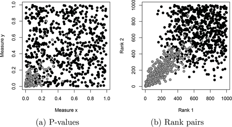
P-values (a), and corresponding rank pairs (b) for 1000 genes, 350 of which are reproducible. Gray points indicate reproducible genes, while black points indicate irreproducible genes. Note that irreproducible genes are generally ranked lower than the reproducible ones.

Genes whose measures indicate the most interest to the researcher, for example those showing strong evidence of differential expression, are said to be “highly ranked”, which means that the numerical values of their ranks are small. That is, the most highly ranked gene in a set has rank 1. Genes with reproducible measurements should be consistently highly ranked for both replicate experiments, and are expected to have positive correlation in their ranks. Genes with irreproducible measurements are assumed to have independent ranks.

The procedure proposed in this article uses the maximum rank for each gene to determine which genes are reproducible. This statistic is defined below:

Definition 1.

$$M_g=\max \left\{R_g^x,R_g^y\right\},\hspace{0.17em}g=1,\dots ,n.$$

Table 1 provides a sample dataset of n = 4 genes to illustrate the calculation of maximum rank statistics. Genes that are consistently highly ranked will have a relatively low value for their maximum rank statistic, while inconsistent or low ranked genes will have higher values. For this reason, choosing a threshold based on the maximum rank has the potential to effectively separate reproducible from irreproducible signals. Figure 2 illustrates the maximum rank statistics and receiver operating characteristic (ROC) curve generated from the same dataset introduced in Figure 1. Because we use values of the maximum rank statistic to determine which genes are reproducible, we call the procedure proposed in this article the “maximum rank reproducibility” (MaRR) procedure.

Table 1.

Sample data, ranks, and maximum rank statistics from four genes, assuming larger values of xg, yg indicate more interest to the researcher.

Index (g)	xg	yg	$\left(R_g^x,R_g^y\right)$	Mg
1	1.0	1.3	(3,2)	3
2	−0.2	0.0	(4,3)	4
3	1.2	−1.0	(2,4)	4
4	2.4	2.2	(1,1)	1

Figure 2.

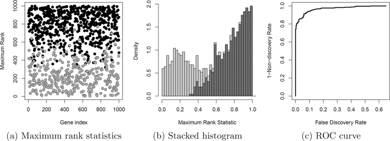
Maximum rank statistics presented two ways, (a) and (b), and corresponding receiver operating characteristic (ROC) curve using M_g as the basis for declaring reproducibility, (c). These figures continue the example from Figure 1. Panel (b) shows a stacked histogram of the maximum rank statistics, illustrating a clear change in behavior between reproducible (light gray) and irreproducible (dark gray) components. It is this transition that we hope to detect using the MaRR procedure.

The joint distribution of all n maximum rank statistics has a complicated covariance structure, as no more than two of these statistics can take on any single value. We can, however, calculate the exact marginal distribution functions for irreproducible genes when certain conditions are in place. We define these conditions in Section 3.1, and present the marginal distribution functions as Proposition 1 and Corollaries 1 and 2.

We now derive the estimator of the proportion of reproducible genes in the sample, ${\pi }_1$, using the MaRR procedure. To derive this estimator and show that it is consistent, we re-scale the maximum rank statistics to the unit interval by considering $M_g/n$. When ${\pi }_1=0$, all n genes are irreproducible and the marginal probability mass function for $M_g/n$ can be calculated exactly.

Proposition 1.

Assume that all n genes are irreproducible. Then the marginal probability mass function for the normalized maximum rank statistic $M_g/n$ is

$$f_{n,0}\left(i/n\right)=\{\begin{array}{ll}\frac{2i-1}{n^2}\hfill & 0<i/n\le 1\hfill \\ 0\hfill & \text{otherwise}\hfill \end{array}.$$

Proof.

See supplementary materials.

3.1. Derivation of Estimate ${\widehat{\mathbf{\pi }}}_{\text{1}}$ Under Ideal Setting

We now derive a procedure to estimate ${\pi }_1$ in an ideal setting by making strong assumptions about the behavior of the marginal ranks $R_g^x$ and $R_g^y$. We later relax these assumptions, discuss the properties of ${\widehat{\pi }}_1$ in realistic settings, and derive estimates for FDR in Section 3.2. We call the setting consistent with the strong assumptions “ideal,” and settings consistent with relaxed assumptions “realistic.” For clarity of notation, we use the index h to indicatea gene that is assumed to have irreproducible measurements.

Assumptions under the ideal setting

(I1) Reproducible signals are always ranked higher than irreproducible signals, that is, $R_g^x<R_h^x$ and $R_g^y<R_h^y$ if gene g is reproducible and gene h is irreproducible.

(I2) The correlation between the ranks of reproducible signals is nonnegative.

(I3) The two ranks per irreproducible gene are independent.

As a result of assumption (I1), $M_g<M_h$ for all reproducible genes g and irreproducible genes h. Letting ${\pi }_1$ be the proportion of reproducible genes, this implies that all genes g such that $M_g/n\le {\pi }_1$ are reproducible, and all genes h such that $M_h/n>{\pi }_1$ are irreproducible. Rank pairs and maximum rank statistics for a sample dataset generated under the ideal assumptions with ${\pi }_1=0.35$ are provided in Figures 3(a) and 3(b). We can now derive the relevant distribution functions for $M_h/n$ when ${\pi }_1>0$. For notational simplicity, define

$$j_{{\pi }_1}=\underset{i=1,\dots ,n}{\max }\left\{i:i/n\le {\pi }_1\right\}=\lfloor n{\pi }_1\rfloor .$$ (1)

In the ideal setting described above, reproducible genes must have maximum ranks no more than $j_{{\text{π}}_1}=\lfloor n{\pi }_1\rfloor$, thus possible values for M_h are $j_{{\pi }_1}+1,\dots ,n$. Adaptation of f_n,0 in Proposition 1 gives the marginal mass function for $M_h/n$ dependent on ${\pi }_1$:

Figure 3.

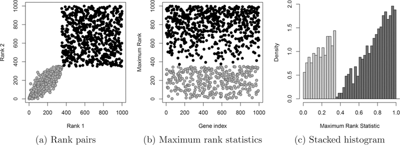
Data from 1000 genes generated under the assumptions for the ideal setting. 350 of these genes (gray) are assumed to be reproducible, and the remaining 650 genes (black) are irreproducible. In this example, there is a sharp transition from reproducible to irreproducible with no overlap. This transition is very apparent in the stacked histogram (c).

Corollary 1.

$$f_{n,{\pi }_1}\left(i/n\right)=\{\begin{array}{ll}\frac{2\left(i-j_{{\text{π}}_1}\right)-1}{{\left(n-j_{{\text{π}}_1}\right)}^2}\hfill & {\pi }_1<i/n\le 1\hfill \\ 0\hfill & \text{otherwise}\hfill \end{array}.$$

As a further result, the marginal cumulative distribution, $F_{n,{\pi }_1}$ and survival, $S_{n,{\pi }_1}$, functions can be calculated.

Corollary 2.

$\text{Let}\hspace{0.17em}{\pi }_1\in \left(0,1\right),x\in \left(0,1\right),i_x=\lfloor nx\rfloor$, and $j_{{\pi }_1}=\lfloor n{\pi }_1\rfloor$. Then the marginal cumulative distribution and survival functions are

$$F_{n,{\pi }_1}\left(x\right)=\{\begin{array}{ll}0\hfill & x<{\pi }_1\hfill \\ \frac{{\left(i_x-j_{{\pi }_1}\right)}^2}{{\left(n-j_{{\pi }_1}\right)}^2}\hfill & {\pi }_1\le x\le 1\hfill \end{array}$$

$$S_{n,{\pi }_1}\left(x\right)=\{\begin{array}{ll}1\hfill & x<{\pi }_1\hfill \\ 1-\frac{{\left(i_x-j_{{\pi }_1}\right)}^2}{{\left(n-j_{{\pi }_1}\right)}^2}\hfill & {\pi }_1\le x\le 1.\hfill \end{array}$$

Proof.

See supplementary materials.

We also derive the limiting marginal distribution of $M_h/n$:

Theorem 1.

Let π₁ ϵ (0, 1) be fixed, and assume (I1), (I2), and (I3). Then as $n\to \infty$ the marginal limiting distributions of the random variable $M_h/n$ are as below

$$F_{n,{\pi }_1}\left(x\right)\to F_{{\pi }_1}\left(x\right)=\{\begin{array}{ll}0\hfill & x<{\pi }_1\hfill \\ \frac{{\left(x-{\pi }_1\right)}^2}{{\left(1-{\pi }_1\right)}^2}\hfill & {\pi }_1\le x\le 1\hfill \\ 1\hfill & 1<x\hfill \end{array},$$

$$S_{n,{\pi }_1}\left(x\right)\to S_{{\pi }_1}\left(x\right)=\{\begin{array}{ll}1\hfill & x<{\pi }_1\hfill \\ 1-\frac{{\left(x-{\pi }_1\right)}^2}{{\left(1-{\pi }_1\right)}^2}\hfill & {\pi }_1\le x\le 1\hfill \\ 0\hfill & 1<x\hfill \end{array}.$$

Proof.

See supplementary materials.

As illustrated above, the theoretical distribution of M_h is determined by the value of ${\pi }_1$, and under the ideal conditions the observed distribution of maximum rank statistics should resemble most closely the theoretical distribution with the correct value of ${\pi }_1$. In practice, the value of ${\pi }_1$ is unknown, thus the MaRR procedure estimates ${\pi }_1$ by comparing observed and theoretical distributions of maximum rank statistics. The estimate for ${\pi }_1$ can thus be chosen as the value that produces the best match between observed and theoretical distributions. A classical approach to this comparison would focus on the cumulative distribution functions. The Cramer–von-Mises statistic (Cramer 1928; von Mises 1931) is a goodness-of-fit statistic that achieves this purpose and is well-known in the change-point literature. In the setting described here, however, the exact distribution of $M_g/n$ is only known for $M_g/n>{\pi }_1$. Using the cumulative distribution function would require assumptions or knowledge about the distribution of maximum rank statistics for reproducible genes. We avoid this issue by using the survival function, allowing consideration of only statistics associated with irreproducible genes. Define the empirical survival function as

$${\widehat{S}}_n\left(x\right)=\frac{1}{n}\sum _{g=1}^{n}I\left(M_g/n\ge x\right),\hspace{0.17em}x\in \left(0,1\right).$$ (2)

We expect the ${\widehat{\pi }}_1$ for which $S_{{\widehat{\pi }}_1}$ is closest to ${\widehat{S}}_n$ to be a consistent estimate for ${\pi }_1$. To define “closest,” we use a weighted mean squared error between the two functions for $\lambda \in \left(0,1\right)$:

Definition 2.

$${\text{MSE}}_n\left(\lambda \right)={\left(n-i_{\lambda }\right)}^{-1}{\sum _{x=i_{\lambda }}^n\left({\widehat{S}}_n\left(x/n\right)-\left(1-\lambda \right)S_{\lambda }\left(x/n\right)\right)}^2,i_{\lambda }=\lfloor \lambda n\rfloor .$$

The definition of ${\text{MSE}}_n\left(\lambda \right)$ includes the factor $\left(1-\lambda \right)$ inside the sum because M_g follows a mixture distribution: $M_g\sim \lambda G+\left(1-\lambda \right)F_{\lambda }$, where G is the unknown distribution of reproducible genes, and $F_{\lambda }$ is defined in Corollary 2. Therefore, the theoretical $S_{\lambda }$ must be normalized by $\left(1-\lambda \right)$. For a finite dataset of size n, ${\text{MSE}}_n\left(\lambda \right)$ can be calculated for any value of $\lambda \in \left(0,1/n,2/n,\dots ,\left(n-1\right)/n\right)$, and we expect it to be small for values of λ close to the true ${\pi }_1$, and larger for values far from ${\pi }_1$. Thus, we define the estimate ${\widehat{\pi }}_1$ in the finite case and show it to be asymptotically consistent below:

Theorem 2.

Let the ideal assumptions hold, and define the estimate ${\widehat{\pi }}_1$ of ${\pi }_1$ as

$${\widehat{\pi }}_1=n^{-1}\underset{i\in \left(0,\dots ,n-1\right)}{\arg \min }\left\{{\text{MSE}}_n\left(i/n\right)\right\}.$$

Then as $n\to \infty$,

$${\widehat{\pi }}_1\stackrel{p}{\to }{\pi }_1.$$

Proof.

See supplementary materials.

Figure 4 illustrates the calculation of ${\widehat{\pi }}_1$ for the sample ranks presented in Figure 3(a). The figure shows that ${\text{MSE}}_n\left(i/n\right)$ is very small near the correct ${\pi }_1$, and for i/n close to 1. It is small for $i/n\in \left(0.9,1\right)$ because this part of the survival function is very similar regardless of the true value of ${\pi }_1$. For this reason, in practice it is necessary to consider only values of ${\widehat{\pi }}_1\in \left(0,.9\right)$. Once ${\widehat{\pi }}_1$ has been determined, it is assumed that gene g is reproducible if $M_g/n\le {\widehat{\pi }}_1$. In the ideal setting, it also means that gene h is irreproducible if $M_h/n>{\widehat{\pi }}_1$. This perfect split, however, only occurs under the ideal assumptions, and we must define an estimate of the false discovery rate for each gene with $M_g/n>{\widehat{\pi }}_1$ for realistic settings. In the next section, we relax the ideal assumptions and derive a false discovery rate estimate.

Figure 4.

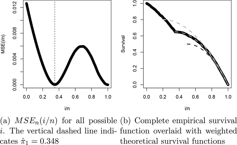
Continuing the example from Figure 3, (a) shows the values of MSE(i/n) for $i=0,1,\dots ,n-1$, and (b) the empirical survival function (solid black) overlaid with the theoretical survival functions (dashed). The theoretical survival functions are generated for $\lambda =0.5$ (dark gray), $\lambda =0.35$ (gray), and $\lambda =0.2$ (light gray). Here, the true ${\pi }_1$ is 0.35, and the estimate is ${\widehat{\pi }}_1=0.348$. It is clear that the empirical survival curve is very similar to the correct theoretical curve.

3.2. Estimation of False Discovery Rates in Realistic Settings

In this section, we make assumptions that are reasonably met by many real datasets, and use them in conjunction with ${\widehat{\pi }}_1$ to estimate marginal false discovery rates of rejection regions for M_g. For a realistic setting, we continue to assume (I2) and (I3) from the ideal setting, but relax (I1):

Assumptions for a realistic setting

(R1) Reproducible signals tend to be ranked higher than irreproducible signals. Thus, if gene g is reproducible and gene h is irreproducible,

$$P\left(R_g^x<R_h^x\right)>1/2,\mathrm{and}P\left(R_g^y<R_h^y\right)>1/2$$

(I2) The correlation between the ranks of reproducible signals is nonnegative.

(I3) The two ranks per irreproducible gene are independent.

The difference between assumptions (R1) and (I1) is the lack of a clear split between reproducible and irreproducible signals in terms of M_g. The estimator ${\widehat{\pi }}_1$ derived in Section 3.1 is consistent in the ideal case, but is conservatively biased in the realistic case: $E\left[{\widehat{\pi }}_1\right]\le {\pi }_1$. We provide a justification of this statement in the supplementary materials and summarize the argument here. In realistic settings, reproducible signals $M_g/n$ have a positive probability of falling in the region $\left({\pi }_1,1\right)$. The smaller the effect size the larger this probability. As a result, the empirical survival curve will take on larger values in the region $\left({\pi }_1,1\right)$ than it would in the ideal case. Weighted theoretical survival $\left(1-\text{λ}\right)S_{\text{λ}}\left(x\right)$ have larger values for smaller values of λ, as illustrated in Figure 4(b), thus the empirical survival curve in the realistic case will be closer to a curve $\left(1-{\text{λ}}^{\ast }\right)S_{\text{λ}\ast }$ than to $\left(1-{\pi }_1\right)S_{{\pi }_1}$ for some ${\text{λ}}^{\ast }\le {\pi }_1$. As a result, the mean squared error will be minimized for some value ${\text{λ}}^{\ast }\le {\pi }_1$, thus $E\left[{\widehat{\pi }}_1\right]\le {\pi }_1$. Figure 5 provides empirical and theoretical survival curves for varying effect sizes to illustrate the estimation of ${\widehat{\pi }}_1$.

Figure 5.

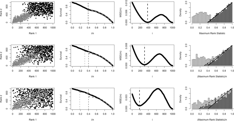
Illustration of MaRR procedure for three datasets of size n = 1000 with 400 reproducible signals: large effect size (row 1), moderate effect size (row 3), and small effect size (row 3). The first column shows rank pairs for both irreproducible (gray) and reproducible (black) signals. The second column presents the corresponding empirical survival curves (black) overlaid with the theoretical survival curve for the true ${\pi }_1=.4$ (dark gray) and the theoretical survival curve for ${\widehat{\pi }}_1$ (light gray). Column three shows the MSE_n curves used to determine $\widehat{k}$ for each dataset. Finally, column four gives the stacked histograms of M_g overlaid with theoretical irreproducible densities $f_{{\widehat{\pi }}_1}$ (dashed) and $f_{{\pi }_1}$ (solid). These densities intersect the x-axis at ${\widehat{\pi }}_1$ and ${\pi }_1$ respectively. As can be seen, the empirical survival curves most closely approximate theoretical curves with ${\widehat{\pi }}_1\le {\pi }_1$ (column 2), and the estimate ${\widehat{\pi }}_1$ marks the approximate beginning of irreproducible signals (column 4).

For convenience, we now move away from the unit interval and work with the originally scaled $M_g=1,\dots ,n$. We therefore define and use the discrete and rescaled version of ${\widehat{\pi }}_1$,$\widehat{k}$

$$\widehat{k}=\underset{i=0,1,\dots ,\lfloor .9n\rfloor }{\arg \min }\left\{{\text{MSE}}_n\left(i/n\right)\right\}.$$ (3)

In practice, we find that $\widehat{k}$ is a good estimate¹ of when reproducible signals begin the transition to irreproducible signals. We base this assertion on observation of a large number of simulated datasets with varying degrees of effect size and proportion of reproducible signals, although it unfortunately cannot yet be proven theoretically. Figure 5 illustrates the performance of $\widehat{k}$ using stacked histograms for a small number of datasets. The figure also includes the corresponding datasets, survival curves, and MSE_n curves to illustrate the estimation of $\widehat{k}$ for varying effect sizes.

To determine the set of reproducible genes we choose a critical value, $\widehat{N}$, according to an error rate, and declare all genes associated with $M_g\le \widehat{N}$ as reproducible. This approach is akin to defining a rejection as $\left(0,\widehat{N}\right)$, and rejecting the null hypothesis of irreproducibility for all signals with M_g in this region (Storey, Taylor, and Siegmund 2004). We use the term “false discovery” to describe the Type 1 error committed when an irreproducible gene is declared reproducible, and estimate a marginal false discovery rate (Genovese and Wasserman 2002) based on a rejection region.

Consider Table 2 detailing possible decision outcomes for m simultaneous hypotheses, where U is the number of true null hypotheses that were correctly not rejected, V is the number of false rejections, T is the number of hypotheses that were not rejected when they should have been, and S is the number of correctly rejected hypotheses. Q is the total number of rejections made. The marginal false discovery rate (mFDR) (Genovese and Wasserman 2002) is thus defined

$$\text{mFDR}\hspace{0.17em}\text{=}\frac{E\left[V\right]}{E\left[Q\right]}.$$ (4)

This quantity is closely related to the classical false discovery rate (FDR) as defined by Benjamini and Hochberg (1995). Related quantities in common usage include the positive FDR (pFDR) (Storey 2002), the irreproducible discovery rate (idr)(Li et al. 2011), and the local false discovery rate (lfdr) (Efron 2004). To describe our approach to mFDR estimation, we introduce the following notation:

$$\begin{gathered} Q\left(i\right)=\sum _{g=1}^{n}I\left(M_g\le i\right)=\#\text{genes}\hspace{0.17em}\text{declared}\hspace{0.17em}\text{reproducible}\hspace{0.17em}\text{for} \\ \hspace{1em}\hspace{1em}\text{critical}\hspace{0.17em}\text{region}\left(0,\text{i}\right) \end{gathered}$$ (5)

$$\begin{array}{l}{V}_k\left(i\right)=\#\hspace{0.17em}\text{irreproducible}\hspace{0.17em}\text{genes}\hspace{0.17em}\text{declared}\hspace{0.17em}\text{reproducible}\\ \hspace{1em}\hspace{1em}\hspace{1em}\text{with}\hspace{0.17em}\text{k}\hspace{0.17em}<M_g\le i.\end{array}$$ (6)

Using this notation, the estimated mFDR for using i as the threshold value for declaring reproducibility is

$$m\widehat{\text{FDR}}\left(i\right)=\frac{E\left[V_{\widehat{k}}\left(i\right)\right]}{Q\left(i\right)}.$$ (7)

The denominator of this expression is determined directly from data, however the numerator must be calculated using the distribution of M_h calculated in Section 3.1, and dependent on $\widehat{k}$. With the value of $\widehat{k}$ determined, all genes with $M_g\le \widehat{k}$ are declared reproducible. Recall that $\widehat{k}$ under-estimates $n{\pi }_1$, thus $n-\widehat{k}$ over-estimates the true number of irreproducible genes. By using this assumption that there are $n-\widehat{k}$ irreproducible genes in the dataset, we calculate $E\left[V_{\widehat{k}}\left(i\right)\right]$ using the cumulative distribution function $F_{n,\widehat{k}/n}$ from Corollary 2.

Table 2.

Decision outcomes for m hypothesis tests.

	Fail to reject null	Reject null	Total
Null is true	U	V	m0
Null is false	T	S	m − m0
Total	m − Q	Q	m

The calculation of the numerator is thus detailed

$$\begin{array}{l}E\left[V_{\widehat{k}}\left(i\right)\right]=\left(n-\widehat{k}\right)\cdot P_{n,\widehat{k}/n}\left(M_h\le i\right)\\ \hspace{1em}\hspace{1em}\hspace{1em}\hspace{1em}=\left(n-\widehat{k}\right)\cdot \frac{{\left(i-\widehat{k}\right)}^2}{{\left(n-\widehat{k}\right)}^2}\\ \hspace{1em}\hspace{1em}\hspace{1em}\hspace{1em}=\frac{{\left(i-\widehat{k}\right)}^2}{n-\widehat{k}},\hspace{1em}i=\widehat{k}+1,\dots ,n.\end{array}$$ (8)

We can then define the estimated mFDR associated with any rejection region (0, i).

$$m\widehat{\text{FDR}}\left(i\right)=\frac{E\left[V_{\widehat{k}}\left(i\right)\right]}{Q\left(i\right)}=\frac{{\left(i-\widehat{k}\right)}^2}{Q\left(i\right)\left(n-\widehat{k}\right)},i=\widehat{k}+1,\dots ,n.$$ (9)

Thus, the false discovery rate is controlled at a nominal level α if the threshold value $\widehat{N}$ is chosen to be

$$\widehat{N}=\underset{\widehat{k}<i\le n}{\max }\left\{i:m\widehat{\text{FDR}}\left(i\right)\le \alpha \right\},$$ (10)

and all genes with maximum rank statistics less than or equal to $\widehat{N}$ are declared reproducible.

We now summarize the maximum rank reproducibility procedure for set of n genes each with two measurements generated from replicate experiments.

MaRR Procedure:

To control FDR at a nominal level of α:

$$\begin{array}{l}\text{Define}\hspace{0.17em}\widehat{k}=\underset{i=0,1,\dots ,\lfloor .9n\rfloor }{\arg \min }\{{\text{MSE}}_n\left(i/n\right)={\left(n-i\right)}^{-1}\sum _{x=i}^n\\ \hspace{1em}\hspace{1em}\hspace{1em}\hspace{1em}\hspace{1em}\times {\left({\widehat{S}}_n\left(x/n\right)-\left(1-i/n\right)S_{i/n}\left(x\right)\right)}^2\},\end{array}$$

where ${\widehat{S}}_n\left(x\right)$ is the empirical survival function, and $S_{i/n}\left(x\right)$ is the limiting survival function defined in Theorem 1. Define $\widehat{N}$ as

$$\widehat{N}=\underset{\widehat{k}<i\le n}{\max }\left\{i:m\widehat{\text{FDR}}\left(i\right)=\frac{{\left(i-\widehat{k}\right)}^2}{Q\left(i\right)\left(n-\widehat{k}\right)}\le \alpha \right\}.$$

where Q(i) is the number of genes with maximum ranks less than or equal to i. Reject all genes g associated with maximum ranks M_g less than or equal to $\widehat{N}$.

4. Simulation Studies

We now describe two sets of simulation studies designed to assess the performance of the MaRR procedure. For both studies we compare our results to those of the copula mixture model of Li et al. (2011). Li et al. compared their method’s performance to that of existing p-value combination techniques such as Fisher’s and Stouffer’s, finding in all cases that their approach offered a clear advantage. Because of these previous results, in these simulation studies we compare the MaRR approach only to the copula mixture model. Both methods perform analysis on the rank scale, negating the need to calculate p-values and allowing the simulations to proceed directly from simulated test statistics.

The first study, simulation A, generates data from the parametric model assumed by the copula mixture model. The purpose of this simulation is to illustrate the performance of the MaRR procedure in situations where the copula mixture model has been shown to be effective. The second study, simulation B, mimics our motivating RNA-seq datasets from the SEQC study. These datasets do not follow the parametric assumptions made in the copula mixture model’s formulation.

4.1. Settings for Simulation A

In the first study, we vary three parameters: the effect size $\left({\mu }_A\right)$, the proportion of reproducible signals $\left({\pi }_1\right)$, and the correlation between these signals $\left(\rho \right)$. We assume that large values of test statistics will be highly ranked, corresponding to calculation of right-tail one-sided p-values. The test statistics for reproducible signals are generated as follows

$$\left(\begin{array}{c}{Z}_{g,1}\\ Z_{g,2}\end{array}\right)\sim N\left(\left(\begin{array}{c}{\mu }_A\\ {\mu }_A\end{array}\right),\left(\begin{array}{cc}1& \rho \\ \rho & 1\end{array}\right)\right).$$ (11)

Irreproducible signals are generated from the standard bivariate normal distribution

$$\left(\begin{array}{c}{Z}_{h,1}\\ Z_{h,2}\end{array}\right)\sim N\left(\left(\begin{array}{c}0\\ 0\end{array}\right),\left(\begin{array}{cc}1& 0\\ 0& 1\end{array}\right)\right).$$ (12)

We let ${\mu }_A\in \left\{1,2,3\right\}$, $\rho \in \left\{0.40,0.85\right\}$, and ${\pi }_1\in \left\{0.10,0.30,0.65,0.80\right\}$, resulting in a total of 24 settings. For each setting, we simulate 100 datasets of size n 2000 and apply both the MaRR procedure and the copula mixture model, controlling error rates at α 0.05. The copula mixture model requires specification of initial parameter values for ${\mu }_A$, $\rho$, $\sigma$, and ${\pi }_1$ to perform an expectation maximization algorithm. We thus performed the procedure ten times on each dataset, drawing initial parameters from uniform distributions with the domains ${\mu }_A\pm 0.50$, $\rho \pm 0.10$, and ${\pi }_1\pm 0.10$. The initial parameter for σ was always set at the true value, $\sigma =1$. Results with the highest likelihood were recorded. For each dataset, we calculate the empirical false discovery rate for each procedure separately by dividing the number of false calls by the total number of genes declared reproducible. The results are presented and discussed in Section 4.3.

4.2. Settings for Simulation B

The objective of the second simulation study is to imitate the observed rank sets from the RNA-seq data analyzed in Section 5, and to further assess the performance of the MaRR procedure. For the RNA-seq datasets the correlation is nearly perfect for the highest ranked signals, but a gradual reduction in correlation is observed for progressively lower ranked genes. In some datasets the correlation remains relatively high (e.g., Figure 9, 1–2), and in others it deteriorates further before the initiation of an irreproducible component (Figure 9, 3).

Figure 9.

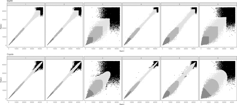
Comparisons for the SEQC data. The rows show decision boundaries for the MaRR procedure (top) and the copula mixture model (bottom). The gray shades from dark to light show the top k transcripts for k 8000, 20,000, and the number of signals declared reproducible by MaRR at α = 0.001, respectively. Black dots indicate transcripts not declared reproducible for any included value of k. Comparisons 1–3 are within-lab and comparisons 4–6 are between-lab, with details described in Table 5.

For each reproducible gene g the first test statistic, $t_{g,1}$ is generated according to $t_{g,1}\sim \text{Unif}\left(1,5\right)$ The correlation between test statistics $t_{g,1}$ and $t_{g,2}$ is linearly dependent on the value of $t_{g,1}$. We assume that for $t_{g,1}=5$ there is perfect correlation, and for the smallest value of $t_{g,1}=1$ the correlation is some reduced value r₀. Given $t_{g,1}$, the remaining test statistic $t_{g,2}$ is assumed to follow a normal distribution

$$t_{g,2}|t_{g,1}\sim N\left(t_{g,1},1-r_g^2\right)$$ (13)

Where $r_g=\frac{1-r_0}{4}\left(t_{g,1}-1\right)+r_0.$

As before, the largest values of $t_{g,1}$, $t_{g,2}$ are considered to be the most highly ranked signals. Irreproducible signals are generated following (12). We include 12 parameter settings for simulation B by varying the proportion of reproducible signals, ${\pi }_1\in \left\{0.10,0.30,0.65,0.80\right\}$ , and the minimum correlation value, $r_0\in \left\{0.30,0.70,0.95\right\}$. For each setting, we generate 100 datasets. To more closely imitate the SEQC data, each dataset has size n = 10,000. As before, we record results from the MaRR procedure and copula mixture model. For the latter, we record the result with the highest likelihood after using ten different initial parameter sets drawn from uniform distributions with domains (2, 3) for ${\mu }_A$, (0.70, 0.99) for $\rho$, and ${\pi }_1\pm 0.10$ for ${\pi }_1$.

4.3. Simulation Results

4.3.1. FDR Control

Figure 6 compares the FDR control for the MaRR procedure and the copula mixture model for data generated using the copula mixture model’s parametric assumptions (Simulation A). Taken as a whole, the results show that MaRR performs well in most situations, and overall is comparable to the copula mixture model. There were two challenging situations for the MaRR procedure. The first situation is when signals are weak and infrequent $\left({\mu }_A=1,{\pi }_1=0.1\right)$. The MaRR procedure was anti-conservative in these settings. This is expected due to the assumption that no irreproducible signals have maximum rank less than $\widehat{k}$, the value at which the MaRR procedure determines irreproducible genes first appear. In this setting, it is likely that some irreproducible maximum ranks are less than $\widehat{k}$, leading to inflated FDR estimates. In the same situation, the copula mixture model is very conservative if the signals are weakly correlated across replicates (ρ = 0.4). In these cases, the real signals may fall in the undetectable regions, which makes identification difficult for any methods (Donoho and Jin 2004). In practice, practitioners who apply MaRR when ${\pi }_1$ is suspected to be very small should be wary of inflated FDR estimates, or they may set $\widehat{k}$ to be zero if they desire strict FDR control. The second situation is when a very large but weakly correlated reproducible group (μ_A =1 or 2, ρ = 0.4, and π₁ = 0.8) is present. In this case, the two components are not well separated and the irreproducible component overwhelms the reproducible component. As a result, the MaRR procedure cannot accurately estimate $\widehat{k}$ based on irreproducible signals, due to overlap with the reproducible component. MaRR systematically underestimates ${\pi }_1$, resulting in an overly conservative decision. In this setting, the copula mixture model is a better choice for inference. This is expected, as these situations are generated from the true models of the copula mixture model. The copula mixture model is expected to be advantageous over nonparametric models in these situations.

Figure 6.

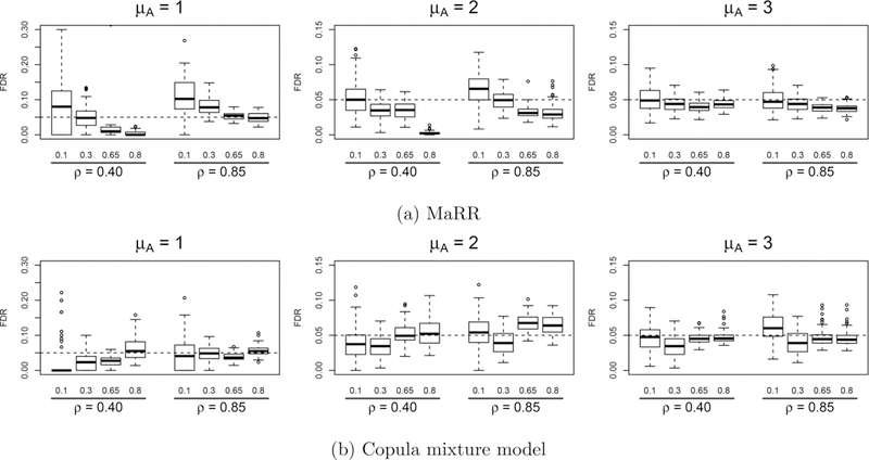
Empirical FDR results for simulation A based on 100 simulated datasets in each setting. The dashed line indicates the target FDR level (0.05) for all simulation . Labels along the x-axis describe values of π₁ (top level) and of ρ (bottom level).

In simulation B (Figure 7), the MaRR procedure effectively controls FDR across all situations examined, with no settings requiring extra care. Both methods tend to be conservative, but the copula model is more conservative when r₀ is 0.95. We will look into this case in more details in the following two subsections.

Figure 7.

FDR results for simulation B based on 100 simulated datasets in each setting. The dashed line indicates the target FDR level (0.05) for all simulations. Labels along the x-axis describe values of π₁ (top level) and method (bottom level).

4.3.2. Discriminative Power

Next, we compare the discriminative power of these two procedures. Figures 8 (a)–(e), shows the discriminative power for three datasets from simulation A and two from simulation B. The two approaches have similar discriminative power in most cases from simulation A with the exception of two situations. The copula mixture model tends to outperform MaRR in the presence of a large and not well-separated reproducible group that overwhelms the irreproducible group. The MaRR procedure tends to have higher discriminative power for settings from simulation B when r₀ = 0.95 and π₁ = 0.80, that is, when the data resemble the distribution of RNA-seq data.

Figure 8.

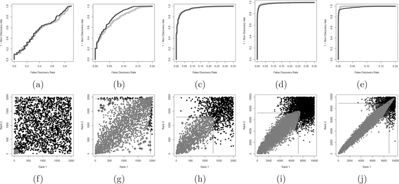
Discriminative (top row) and corresponding decision boundaries (bottom row) for representative datasets from simulations A and B. Top row, right and dark gray curves were calculated using the MaRR procedure and the copula mixture model respectively. In the bottom row, lines outline the square decision boundary of the MaRR procedure, and gray dots illustrate the decision boundary of the copula mixture model. The gray dots above and to the left of the lines are signals found to be reproducible by the copula model but not the MaRR procedure. Crosses are signals declared reproducible for the MaRR procedure but not for the copula model. From left to right: (a) and (f ) follow setting A with μ_A = 1, π₁ = 0.1, ρ = 0.85; (b) and (g) follow setting A with μ_A = 1, π₁ = 0.8, ρ = 0.85; (c) and (h) follow setting A with μ_A = 2, π₁ = 0.65, ρ = 0.85; (d) and (i) follow setting B with r0 = 0.7, π₁ = 0.65; (e) and (j) follow setting B with r₀ = 0.95, π₁ = 0.80.

4.3.3. Decision Boundary

We now compare the decision boundaries of the two methods and show that the decision boundary of MaRR is more desirable for the application of RNA-seq data. The decision boundary determines how the reproducibility of relatively low abundance signals is prioritized. It is particularly relevant to RNA-seq data, as many functionally important genes have a low abundance and the information on their reproducibility is especially helpful for establishing confidence in their measurements (Roberts and Pachter 2011; Mercer et al. 2012).

MaRR always has a consistent, square decision boundary, while that of the copula mixture model has a shape similar to a bivariate Gaussian tail and is influenced by the empirical distribution of the reproducible component. For data that behaves as in Figure 8(i), the two methods give very similar results. In the case of Figure 8(j), the parametric decision boundary is overly narrow and extends well into the irreproducible component, causing an omission of reproducible signals that are somewhat off diagonal y = x. This behavior is related to the parametric assumption of the copula mixture model, which we discuss in detail in Section 5.3. The nonparametric nature of the MaRR procedure is likely to improve analysis for this type of situation.

These simulation results, ROC curves, and decision bound-aries show two primary facts. First, the MaRR procedure performs well in most situations in our simulations, with care needed primarily when the proportion of reproducible signals is small or when there is no obviously irreproducible component. Second, the MaRR procedure has favorable performance in situations similar to those in Figure 8(j), when correlation of reproducible signals is nearly perfect for the highest ranked signals and erodes only slightly for progressively lower ranked ones. This second fact further motivates the use of the MaRR procedure for the SEQC data.

5. Application to SEQC Data

To illustrate the utility of the MaRR procedure, we apply it to the problem of assessing reproducibility of RNA-seq data. We use data produced for the Sequencing Quality Control project to compare and evaluate three RNA-sequencing platforms across different labs using Universal Human Reference RNA samples.

Section 5.1 discusses the data, its read depth, and the processing necessary to perform the MaRR procedure. We present results in Section 5.2 for two types of comparisons: (1) biological replicates from the same lab, and (2) biological replicates from different labs using the same platform. We perform the same comparisons using the copula mixture model. Finally, we discuss and evaluate the findings in Section 5.3.

5.1. Data

The Universal Human Reference RNA sample was sequenced by all 13 laboratories involved in the SEQC project. The Mayo Clinic, BGI, Cornell, City of Hope, Novartis, and the Australian Genome Research Facility used Illumina HiSeq 2000. Penn State, Northwestern, SeqWright Inc., and Liverpool used Life Technologies. Finally, Roche 454 data were produced by the Medical Genomes Project, New York University Medical Center, and SeqWright Inc.

We apply the MaRR procedure and copula mixture model to measure reproducibility within labs and between labs. For within-lab comparisons, we rank and compare transcripts from replicates produced by the Mayo Clinic (Mayo), Penn State (PSU), and New York University Medical Center (NYU). Table 3 summarizes these replicates and their corresponding read depths. To make comparisons between labs using the same technology, we sum read counts over all replicates per lab. We then rank the total read counts for each lab and make three comparisons: Illumina, Life Technologies, and Roche 454. Table 4 summarizes which labs were selected, the number of replicates per lab, and the read depth.

Table 3.

Summary of sequencing platform, laboratories, and read depth for replicates used for within-lab comparisons. Differences in read depth may be due to the sequencing technologies or be a choice made by individual labs.

Technology	Laboratory	Read depth
Illumina	Mayo	152,240,873
	Mayo	288,049,574
Life Technologies	PSU	92,762,967
	PSU	96,634,448
Roche 454	NYU	610,609
	NYU	666,621

Table 4.

Summary of sequencing technology, laboratories, and read depth for datasets used for between-lab comparisons. Roche 454 produces far fewer reads than Illumina and Life Technologies, however these reads are significantly longer.

Technology	Laboratory	Replicates	Read depth
Illumina	Mayo	4	1,141,566,965
	BGI	5	1,008,962,065
Life Technologies	PSU	5	400,076,114
	NWU	5	517,881,698
Roche 454	NYU	2	1,277,230
	SQW	2	1,139.842

For all comparisons, highly ranked transcripts are those with the most read counts. Ranking ties are treated by random assignment. For example, if two transcripts are tied with three transcripts ranked higher than both, one of the tied transcripts is randomly assigned the rank of four and the remaining transcript the rank of five. The technologies have varying read depth, but the reads are all mapped to the same set of 43,919 transcripts. Increased read depth for Illumina and Life Technologies experiments appears to affect the reproducibility of results, as we discuss in more detail in Section 5.3.

After an initial examination of all six comparisons, we found that the distribution of ranked read counts shows very high correlation for the most highly ranked transcripts, with a gradual deterioration in correlation for less highly ranked transcripts. Additionally, we found that for all comparisons of interest there was an obvious irreproducible component, meeting the requirements of the MaRR procedure.

For external validation of results, we use the Taqman polymerase chain reaction (PCR) data associated with the SEQC project. Expression levels measured with PCR are typically viewed as a reference “gold” standard. For this reason, we use the PCR values as a benchmark for objectively assessing the performance of both procedures with the SEQC data. The PCR experiments were done on the same RNA sample as the RNA-seq data, each with four technical replicates. They were mapped to 1129 transcripts in the SEQC data. We average the PCR values over the four replicates and rank them based on this average. We discuss results using these PCR ranks in Section 5.3.

5.2. Analysis and Results

We applied both procedures to each of six comparisons. The copula mixture model was performed ten times with different starting values to ensure convergence. Results with the highest likelihood are reported. We provide the number of signals declared reproducible at an estimated error rate of α = 0.01, the estimated proportion of reproducible signals, ${\widehat{\pi }}_1$, and the correlation for transcripts declared reproducible, $\widehat{\rho }$. The results are summarized in Table 5 and illustrated in Figure 9.

Table 5.

Summary of results for RNA-seq comparisons. (1, 2, 3) correspond to comparisons within labs, and (4, 5, 6) to comparisons between labs. The columns in each results section give the estimated proportion of reproducible signals, the correlation for transcripts declared reproducible, and the number of transcripts declared reproducible using an error threshold of α = 0.01.

			MaRR results			Copula results
Comparison	Tech	Labs	${\widehat{\pi }}_1$	$\widehat{\rho }$	$\widehat{\text{FDR}}<.01$	${\widehat{\pi }}_1$	$\widehat{\rho }$	$\text{IDR<0}.01$
1	Illumina	Mayo	0.851	0.998	38975	0.773	0.999	33902
2	Life	PSU	0.847	0.997	38778	0.767	0.999	32809
3	Roche	NYU	0.566	0.889	27020	0.551	0.904	23130
4	Illumina	Mayo and BGI	0.900	0.998	40855	0.861	0.997	38039
5	Life	PSU and NWU	0.898	0.989	40760	0.649	0.904	27937
6	Roche	NYU and SQW	0.606	0.843	28798	0.620	0.859	26376

5.3. Discussion

The results reported in the previous section show a very high level of reproducibility for the Illumina and LIFE technologies, agreeing with the findings of the SEQC project (SEQC/MAQC-III Consortium 2014). For all platforms considered, the estimated proportion of reproducible signals $\left({\widehat{\pi }}_1\right)$ is alarger for between-lab comparisons than for within-lab replicates, although agreement between highly ranked transcripts $\left(\widehat{\rho }\right)$ is somewhat reduced (Table 5). We suspect the larger proportion of reproducible transcripts is due to increased read depth from combination of biological replicates, and the decreased correlation is due to increased noise from between labs. For Illumina this decrease is very slight, while it is most noticeable for the Roche 454 platform whose measurements were the noisiest to begin with. There seems to be a strong relationship between read depth and reproducibility; higher read depth is associated with more reproducible findings. The Illumina platform in particular has almost perfect correlation between ranks for both within and between lab comparisons. The Roche 454 technology, which has far fewer reads per transcript, shows a lower level of both reproducibility and correlation between ranks of reproducible transcripts.

An important part of the analysis is to identify reproducible transcripts. Though reproducibility is less an issue for highabundance transcripts, as they usually are highly reproducible (Figure 9), more uncertainty is present for low-abundance transcripts, as RNA-seq technology has larger variance for low read counts (Love, Huber, and Anders 2014; Zhao et al. 2014). Nevertheless, many low-abundance transcripts, for example, long intergenic non-coding transcripts (lncRNAs), are crucial in defining cellular function in normal and disease states (Roberts and Pachter 2011). The consistency across replicates greatly helps differentiate them from noise. When applied to the SEQC data, both methods give similar results for two of the six comparisons (Roche technology, comparisons 3 and 6), however they differ in both estimates of ${\widehat{\pi }}_1$ and the shape of decision boundary for the remaining comparisons (1, 2, 4, 5). The MaRR procedure found very high proportions of reproducible signals for these comparisons $\left({\widehat{\pi }}_1=0.851,0.847,0.900,0.898\right)$ while the copula mixture model estimated ${\widehat{\pi }}_1$ to be 0.773, 0.767, 0.861, and 0.649, respectively. Here, we compare their decision boundaries, which determine how reproducible signals are identified among weak signals, i.e., the low-abundance transcripts. To display the behavior at different abundance levels, we compare decision boundaries for top-k transcripts, with k = 8000, 20,000 and the number of signals declared reproducible by MaRR at α = 0.01, to reflect descending abundance. The value of the last k varies in each comparison (k = 38,975, 38,778, 27,020, 40,855, 40,760, 28,798 for comparisons 1–6, respectively). The decision boundary at this k reflects the behavior at the cutoff.

For k 8000 and 20,000, the two approaches are in close agreement (Figure 9 dark and intermediate gray). However, when k is large (k > 30,000), the decision boundaries differ: MaRR retains its characteristic square shape, whereas the decision boundaries for the copula mixture model are very “pointy” on the right end for the comparisons with Illumina and Life technology, similar to the results of Simulation B with r₀ = 0.95 and π₁ = 0.80 (Figure 8(j)). This effect is caused by the model’s assumptions that the data’s dependence structure follows a mixture of Gaussian copulas. Due to the symmetry of the Gaussian copula, the right tail of the reproducible component in the copula mixture model tends to mirror the shape of the left tail. When top signals are highly correlated, like in these four cases, the right tail of the reproducible signals, that is, the decision boundary, tends to be pointy, showing a strong favoritism to consistent low signals over signals that have higher signals but are slightly less consistent. For transcripts with low abundance, this decision boundary becomes more extreme, with only the ranks located along the diagonal being deemed reproducible, ignoring some transcripts that have low abundance but are still reasonably consistent across replicates. This effect is especially noticeable in the between-lab comparisons (4–5 in Figure 9), where some signals that are highly ranked in both labs are still deemed irreproducible. On the other hand, MaRR’s square decision boundary prioritizes transcripts that are higher ranked but somewhat off-diagonal over lower ranked transcripts that are very close to the line y = x. As low-abundance transcripts usually have higher dispersion for RNA-seq data (Love, Huber, and Anders 2014; Zhao et al. 2014), real transcripts with low counts are more likely to be somewhat off the diagonal than the highly abundant ones. A square decision boundary is more likely to accommodate these transcripts than a pointy one.

To evaluate which decision boundary is more biologically relevant for these particular data, we consider the Taqman PCR data as a source of external validation. Although PCR measurements are only available for a small subset of the genes considered in the RNA-seq datasets (1129 out of more than 40,000 transcripts), they still provide some insight. Specifically, we compare the PCR genes included in the “top k” signals from one approach but not the other. The PCR genes with smaller rank values would be considered more desirable to identify, as their average expression level is higher. Figure 10 summarizes ranks of procedure-specific PCR genes from the top k genes in each comparison, where k is determined by the number of transcripts declared reproducible by the MaRR procedure for α 0.01. At this k, both methods identify most of the PCR genes. The numbers of commonly identified PCR genes are 1101, 1099, 851, 1120, 1119, and 877 for comparisons 1–6, respectively. In all the comparisons, MaRR identifies more PCR genes than the copula mixture model. Among them, in comparisons 4–5, MaRR identifies all PCR genes identified by the copula mixture model and some additional PCR genes. For most of the rest of comparisons (comparison 1–3), MaRR-specific PCR genes tend to have smaller ranks in PCR measurements than copula-specific genes. Two-sample t-tests to compare the mean rank of method-specific genes yield p-values of 0.0227, 0.0047, 0.2176, and 0.1235 for comparisons 1, 2, 3, and 6, respectively.

Figure 10.

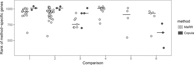
Rank of method-specific PCR genes in the top k for only MaRR (light gray) or for only the copula mixture model (dark gray) for comparisons 1–6. Horizontal lines indicate median values. Here, k is determined by the number of transcripts declared reproducible by the MaRR procedure for α = 0.01. PCR genes with lower-valued ranks are more highly expressed. In all comparisons, more PCR genes are identified only by the MaRR procedure than the copula mixture model. For comparisons 4 and 5, there were no PCR genes identified only by the copula mixture model.

6. Concluding Remarks

In this article, we have introduced MaRR, a nonparametric approach to detect reproducible transcripts from replicate experiments. The MaRR approach is applicable for many different measurement types, makes very few assumptions about the distribution of reproducible signals, and does not rely on tuning parameters or require starting values. Its decision boundary naturally accommodates the elevated dispersion among less highly ranked genes. It works especially well when there is a gradual deterioration in correlation for less highly ranked genes, a situation that is encountered in certain high-throughput data analyses such as RNA-seq data.

Despite these advantages, there are alsoa few caveats to keep in mind when applying the MaRR procedure. Most notably, caution is required when the proportion of reproducible signals is small. In this situation, the estimated FDR may be inflated if there are irreproducible signals with maximum ranks less $\widehat{k}$, the estimated lower bound for irreproducible signals. It is also important that the ranks in the irreproducible component are independent, otherwise the assumptions of the MaRR procedure are not met and conclusions may not be valid. For example, if there is a systematic bias in both replicates that impose a positive correlation structure in the irreproducible component then ${\widehat{\pi }}_1$ tends to overestimate the proportion of reproducible signals.

An extension of the MaRR procedure for simultaneous consideration of more than two replicates is a topic for future research. Although defining what “reproducible” means is complicated in higher dimensions, it is closely related to the partial conjunction hypothesis discussion of Benjamini and Heller (2008). Consider the case of three biological replicates. We then have three ranks for each gene g:$R_g^x$, $R_g^y$, and $R_g^z$. An enhanced MaRR procedure would define a summary rank statistic depending on how “reproducible” is defined. Either the maximum order statistic, $M_g^{\left(3\right)}=\max \left\{R_g^x,R_g^y,R_g^z\right\}$, or the second order statistic $M_g^{\left(2\right)}$ could be used. The marginal distribution of both can be calculated exactly in a derivation similar to that of $f_{{\pi }_1}$ in this article, and corresponding estimates for ${\pi }_1$ and mFDR could be derived. We have outlined the process for $M_g^{\left(3\right)}$ in supplemental materials. This straightforward extension requires tedious algebra, but the resulting procedure will have a closed form solution and fast computation. These approaches are scalable as the dimension increases, due to the effective collapse of high-dimensional ranks into single summary rank statistics.

References

- Benjamini Y, and Heller R (2008), “Screening for Partial Conjunction Hypotheses,” Biometrics, 64, 1215–1222. [1039] [DOI] [PubMed] [Google Scholar]
- Benjamini Y, and Hochberg Y (1995), “Controlling the False Discovery Rate: A Practical and Powerful Approach to Multiple Testing,” Journal of the Royal Statistical Society, Series B, 57, 289–300. [1033] [Google Scholar]
- Boulesteix A-L, and Slawski M (2009), “Stability and Aggregation of Ranked Gene Lists,” Briefings in Bioinformatics, 10, 556–568. [1028] [DOI] [PubMed] [Google Scholar]
- Cramer H (1928), “On the Composition of Elementary Errors,” Scandinavian Actuarial Journal, 1928, 141–180. [1030] [Google Scholar]
- Donoho D, and Jin J (2004), “Higher Criticism for Detecting Sparse Heterogeneous Mixtures,” Annals of Statistics, 32, 962–994. [1034] [Google Scholar]
- Efron B (2004), “Large-Scale Simultaneous Hypothesis Testing: The Choice of a Null Hypothesis,” Journal of the American Statistical Association, 99, 96 [1033] [Google Scholar]
- Genovese C, and Wasserman L (2002), “Operating Characteristics and Extensions of the False Discovery Rate Procedure,” Journal of the Royal Statistical Society, Series B, 64, 499–517. [1032] [Google Scholar]
- Li Q, Brown JB, Huang H, and Bickel PJ (2011), “Measuring Reproducibility of High-Throughput Experiments,” Annals of Applied Statistics, 5, 1752–1779. [1028,1033] [Google Scholar]
- Love MI, Huber W, and Anders S (2014), “Moderated Estimation of Fold Change and Dispersion for RNA-Seq Data with Deseq2,” Genome Biology, 15, 550 [1037] [DOI] [PMC free article] [PubMed] [Google Scholar]
- Mercer TR, Gerhardt DJ, Dinger ME, Crawford J, Trapnell C, Jeddeloh JA, Mattick JS, and Rinn JL (2012), “Targeted RNA Sequencing Reveals the Deep Complexity of the Human Transcriptome,” Nature Biotechnology, 30, 99–104. [1035] [DOI] [PMC free article] [PubMed] [Google Scholar]
- Roberts A, and Pachter L (2011), “RNA-Seq and Find: Entering the RNA Deep Field,” Genome Medicine, 3, 74 [1035,1037] [DOI] [PMC free article] [PubMed] [Google Scholar]
- SEQC/MAQC-III Consortium (2014), “A Comprehensive Assessment of RNA-Seq Accuracy, Reproducibility and Information Content by the Sequencing Quality Control Consortium,” Nature Biotechnology, 32, 903–914. [1029,1037] [DOI] [PMC free article] [PubMed] [Google Scholar]
- Shabtai D, Glaever G, and Nislow C (2012), “An Algorithm for Chemical Genomic Profiling that Minimizes Batch Effects: Bucket Evaluations,” BMC Bioinformatics, 13, 245 [1028] [DOI] [PMC free article] [PubMed] [Google Scholar]
- Storey JD (2002), “A Direct Approach to False Discovery Rates,” Journal of the Royal Statistical Society, Series B, 64, 479–498. [1033] [Google Scholar]
- Storey JD, Taylor JE, and Siegmund D (2004), “Strong Control, Conservative Point Estimation and Simultaneous Conservative Consistency of False Discovery Rates: A Unified Approach,” Journal of the Royal Statistical Society, Series B, 66, 187–205. [1032] [Google Scholar]
- von Mises R (1931), “Wahrscheinlichkeitsrechnung und Ihre Anwendung in der Statistik und Theoretischen Physik,” Leipzig: Deuticke [1030] [Google Scholar]
- Zhang M, Zhang L, Zou J, Yao C, Xiao H, Liu Q, Wang J, Wang D, Wang C, and Guo Z (2009), “Evaluating Reproducibility of Differential Expression Discoveries in Microarray Studies by Considering Correlated Molecular Changes,” Bioinformatics, 25, 1662–1668. [1028] [DOI] [PMC free article] [PubMed] [Google Scholar]
- Zhang Y, Lin Y-H, Johnson TD Rozek LS, and Sartor MA (2014), “PePr: A Peak-Calling Prioritization Pipeline to Identify Consistent or Differential Peaks from Replicated ChIP-Seq Data,” Bioinformatics, 30, 2568–2575. [1028] [DOI] [PMC free article] [PubMed] [Google Scholar]
- Zhao S, Fung-Leung W-P, Bittner A, Ngo K, and Liu X (2014), “Comparison of RNA-Seq and Microarray in Transcriptome Profiling of Activated T Cells,” PloS One, 9, e78644 [1037] [DOI] [PMC free article] [PubMed] [Google Scholar]
Associated Data
This section collects any data citations, data availability statements, or supplementary materials included in this article.