Constructing Precisely Computing Networks with Biophysical Spiking Neurons

Abstract

While spike timing has been shown to carry detailed stimulus information at the sensory periphery, its possible role in network computation is less clear. Most models of computation by neural networks are based on population firing rates. In equivalent spiking implementations, firing is assumed to be random such that averaging across populations of neurons recovers the rate-based approach. Recently, however, Denéve and colleagues have suggested that the spiking behavior of neurons may be fundamental to how neuronal networks compute, with precise spike timing determined by each neuron's contribution to producing the desired output (Boerlin and Denéve, 2011; Boerlin et al., 2013). By postulating that each neuron fires to reduce the error in the network's output, it was demonstrated that linear computations can be performed by networks of integrate-and-fire neurons that communicate through instantaneous synapses. This left open, however, the possibility that realistic networks, with conductance-based neurons with subthreshold nonlinearity and the slower timescales of biophysical synapses, may not fit into this framework. Here, we show how the spike-based approach can be extended to biophysically plausible networks. We then show that our network reproduces a number of key features of cortical networks including irregular and Poisson-like spike times and a tight balance between excitation and inhibition. Lastly, we discuss how the behavior of our model scales with network size or with the number of neurons “recorded” from a larger computing network. These results significantly increase the biological plausibility of the spike-based approach to network computation.

SIGNIFICANCE STATEMENT We derive a network of neurons with standard spike-generating currents and synapses with realistic timescales that computes based upon the principle that the precise timing of each spike is important for the computation. We then show that our network reproduces a number of key features of cortical networks including irregular, Poisson-like spike times, and a tight balance between excitation and inhibition. These results significantly increase the biological plausibility of the spike-based approach to network computation, and uncover how several components of biological networks may work together to efficiently carry out computation.

Introduction

Neural networks transform their inputs through a variety of computations from the integration of stimulus information for decision-making (Gold and Shadlen, 2007) to the persistent activity observed in working memory tasks (Jonides et al., 2008). How such transformations occur in biological networks has not yet been understood. Such operations have been proposed to be performed by the averaged firing rates of neurons in a network (a “rate model”; Seung, 1996; Wang, 2002; Goldman et al., 2003; Machens et al., 2005; Wong and Wang, 2006). For example, persistent activity may be realized in a rate model by including recurrent connections that balance the intrinsic leak of the system (Seung, 1996; Goldman, 2009). However, most real neural circuits consist of spiking neurons. Spiking network implementations of rate model operations can be constructed by assuming that the computation is distributed among a large population of functionally similar neurons, so that the averaged firing rate matches that of the desired rate model (Renart et al., 2004; Wong and Wang, 2006; Eckhoff et al., 2011).

Rate-based approaches have been used to model a variety of behaviors including persistent activity in the oculomotor integrator (Seung, 1996; Seung et al., 2000; Goldman et al., 2003), decision-making (Usher and McClelland, 2001; Bogacz et al., 2006; Wong and Wang, 2006; Eckhoff et al., 2011; Cain and Shea-Brown, 2012), and working memory (Brody et al., 2003; Renart et al., 2004). Although rate models capture features of both psychophysical and electrophysiological data, such approaches have a few potential limitations. First, any rate-based approach disregards the timing of individual spikes, and hence any capacity to compute that precise timing may confer. Second, the performance of rate models is typically quite sensitive to the choice of connection weights between neural populations (Seung et al., 2000). If the recurrent connections are either too strong or too weak, the activity of the network can either quickly increase to saturation or decrease to a baseline level. Further, spiking network implementations of rate-based networks typically (though not always; Lim and Goldman, 2013) require strong added noise to match the irregular firing observed in cortical networks (Wang, 2002; Machens et al., 2005; Wong and Wang, 2006). This injected noise often dominates the feedforward or intrinsic currents generated in the network, diminishing the accuracy with which inputs can be integrated or maintained over time.

Recently, Boerlin et al. (2013) have proposed a distinct alternative by assuming that a computation is performed directly by the spike times of individual neurons. Based upon the premise that the membrane potentials of neurons in the network track a prediction error between a desired output and the network estimate, and that neurons spike only if that error exceeds a certain value, Boerlin et al. (2013) derived a spiking neural network that can perform any linear computation. In this predictive coding approach, the computation error is mapped to the voltage of integrate-and-fire (IF) neurons, whereas a bound on this error is mapped to the neuron's threshold. This leads to a recurrent network of IF neurons with a mixture of instantaneous and exponential synapses that is able to reproduce many features of cortical circuits while performing a variety of linear computations including pure and leaky integration, differentiation, and transforming inputs into damped oscillations. Furthermore, as the computation is efficiently distributed among the participating neurons, the network is robust to perturbations such as lesions and synaptic failure.

Nevertheless, two components of this work potentially limit its implementation in biological networks: neurons communicate instantaneously, whereas true synaptic dynamics occur with a finite timescale; and the threshold of IF neurons is set arbitrarily, rather than being established by intrinsic nonlinear spike-generating kinetics.

Here, starting from the same spike-based framework (Boerlin et al., 2013), we derive a computing network of neurons with standard spike-generating currents (Hodgkin and Huxley, 1952) and synapses with realistic timescales. Like in many cortical networks, the spike times of the model network are irregular and there is a tight balance between excitation and inhibition (Shadlen and Newsome, 1998; Okun and Lampl, 2008; Renart et al., 2010). Moreover, the precise timing of spikes is important for accurate decoding: the network actively produces correlations in the spike times of different neurons, which act to reduce the decoding variance. Together, the results uncover how several components of biological networks may work together to efficiently carry out computation.

Materials and Methods

Optimal spike-based computation with finite time-scale synapses.

Here, we follow Boerlin et al. (2013) to construct a spiking network that implements the computation of a J-dimensional linear dynamical system. We define the target system as follows:

where x(t) is a J-dimensional vector of functions of time, c̄(t) is a J-dimensional vector of stimulus inputs, and A is a J × J matrix (with units of s⁻¹) that determines the linear computation. For example, if A is the zero matrix, then the computation would be pure integration with x(t) being the integral of the stimulus inputs c̄(t). The dynamic variables x are unitless, whereas time has units of seconds. We want to build a network of N neurons such that an estimate of the dynamic variable x̂ ≈ x can be read out from the network's spike trains ρ_k(t) = ∑_jδ(t − t_j^k), where k indexes the N neurons. We assume that the dynamics of the network estimate x̂ are given by the following:

where h_r(t) = (a_r − a_d)/α*H(t)e^−a_rt, H(t) is the Heaviside function, a_r, a_d, and α* are constants that are defined below, and Γ is a J × N dimensional decoding matrix. In the original leaky-integrate-and-fire (LIF) network (Boerlin et al., 2013), h_r(t) = δ(t). The solution of Equation 2, assuming that x̂(0) = 0, is given by the convolution of the network's spike trains with a double-exponential function as follows:

where

and α* is a constant so that the maximum of the double-exponential function is 1, a_r (a_d) is the rate of rise (decay) of the double-exponential function. Note that the normalization term (a_r − a_d)/α* in the definition of h_r(t) comes from the fact that we wanted α(t) to have the form given above. In what follows, we will show that this alteration to the decoder dynamics will result in a neuronal network with finite timescale synapses.

We now derive network dynamics such that neurons spike to reduce the error between the signal x(t) and the estimate x̂(t). Defining the error function E(t) as follows:

our goal is to derive conditions under which cell k spikes only if the error is reduced by doing so: E(t|cell k spikes) < E(t|cell k doesn′t spike). When cell k spikes at time t, this changes x̂_j(u)→x̂_j(u) + Γ_jkα(u − t). Thus, we need to find conditions such that:

Up to this point, our derivation is nearly identical to that of Boerlin et al. (2013), except for the use of the double-exponential function synapse. However, we must now alter the above condition to account for the fact that the double-exponential function synapse has a finite rise time. More specifically, because α(t) is equal to zero at the time of the spike, the terms on either side of the above inequality are equal (because α(u − t) = 0 for u ≤ t). In contrast, Boerlin et al. (2013) used exponential synapses which have an infinitely fast rise time and thus yield a non-zero contribution at the time of a spike. Thus, to account for the effects of the spike at time t on the error, we need to extend the integration a short time t* into the future as follows:

After some algebra, and using the fact that α(u − t) = 0 for u ≤ t, this leads to:

Because t* is assumed to be small, we approximate the above integral using the trapezoidal rule:

Other integral approximations lead to similar results. Using the fact that t* is small, we can Taylor expand x_j(t + t*) and x̂_j(t + t*) to first order:

where we used the fact that α(0) = 0. Dividing both sides of the above equation by α(t*)t* we arrive at:

Lastly, we drop terms of order t* and define:

with the condition that neuron k spikes when it reaches threshold:

The network dynamics are given by differentiating Equation 12:

To close the problem using only information available to the network, we replace the desired signal with the spike-based estimate of the signal, x(t) ≈ x̂(t):

𝕀_J×J is the J-dimensional identity matrix. The above form highlights the fact that there are now two different kinds of synapses in our network: double-exponential “slow” synapses and exponential “fast” synapses. The reason why these two types of synapses arise is because both x̂(t) and its temporal derivative appear in the equation for the voltage dynamics. If we had chosen to decode the spike trains using an exponential kernel as in Boerlin et al. (2013), we would end up with exponential slow synapses and δ-function fast synapses.

In previous approaches, the neurons' voltage “reset” following spikes arose from autaptic (i.e., from a neuron to itself) input currents via the delta-function synapses just discussed. Such fast synapses do not occur in our derivation. To obtain an analogous reset condition, we would need to include an additional, explicit reset current in our voltage equation. This would result in the following:

where the term −2T_kρ_k(t) resets neuron k to −T_k once it reaches threshold T_k. We illustrate this particular reset rule because it matches that of Boerlin et al., (2013). However, in the next section we will remove this reset term and replace it with more biologically realistic ionic currents.

Next, we rescale the voltage to be in terms of millivolts (recall that time is in units of seconds). To do so, we introduce the scaling Ṽ_k = T_k V_k/g (where g has units of millivolts) which leads to the following:

where the threshold voltage is g and the reset voltage is −g. The parameter g also modifies the gain of the synaptic input. However, it is also linked to the value of the voltage threshold and reset potential. Finally, to frame the network equations in terms of current, we multiply both sides by the membrane capacitance C_m (in units of mF/cm²).

Addition of biophysical currents.

We began by deriving a network of neurons that do not contain any intrinsic biophysical currents and solely integrate their synaptic input before spiking. To incorporate the nonlinear dynamics of spike-generating ion channels, we now replace the reset currents −2C_mgρ_k(t) with generic Hodgkin–Huxley-type (HH-type) ionic currents I_ion(V_k, w⃗_k) (see Models and parameters for a specific example):

where the w⃗_k in I_ion(V_k, w⃗_k) represent the gating variables for standard HH currents. For example, w⃗_k = [m_k, h_k, n_k] for the HH-type model we consider here (see Models and parameters). For simplicity, we assume that every neuron in the network has the same type of spike-generating currents I_ion(V_k, w⃗_k). Note that if we wanted to use a leaky-integrate-and-fire neuron, we would set I_ion(V_k, w⃗_k) = − g_L(V_k − E_L) − 2gC_m ρ_k(t), where g_L is the conductance of the leak channel (in mS/cm²), E_L is the leak channel reversal potential, and we used the same reset current we previously described. As stated above, for standard HH-type model currents there is no longer a need for a reset current as the spiking process is performed by the intrinsic currents.

Next, we add a white noise current to our voltage equations. This is meant to roughly model a combination of background synaptic input, randomness in vesicle release, and stochastic fluctuations in ion channel states (channel noise), but also contributes to computation in our networks by helping to prevent synchrony (see Results, Sensitivity to variation in synaptic strength and noise levels). The result is as follows:

where ξ(t) is white noise 〈ξ(t)〉 = 0 and 〈ξ(t)ξ(t′)〉 = δ(t − t′) and σ_V has units of μA/cm² · $\sqrt{s}$. Last, to emphasize the fact that the input to the system c̄(t) has the physical interpretation of current, we introduce the scaling c̄(t) = c(t)/(C_mc₀) where c(t) has units of μA/cm², and c₀ has units of millivolts and scales the stimulus input into neurons in our network. Thus, we rewrite Equation 20 as follows:

Switching to vector notation, the population dynamics are given by the following:

where T̃ is an N × N diagonal matrix with T_k on the diagonal.

In the integrate-and-fire network, spiking occurs due to an explicit threshold crossing and reset condition. With the addition of ionic currents, action potentials are now intrinsically generated, but it is still necessary to identify a voltage threshold for spike times. We treat this detection threshold as a separate parameter. In the simulations presented, we chose to use V_th = −48 mV, which is sufficiently high on the upswing of the action potential to allow reliable spike detection. However, different choices for V_th can lead to different behaviors for the network. In particular, our simulations show that to use a larger value for V_th, one must also increase the voltage noise to prevent the network from synchronizing.

Compensating for spike-generating currents.

In the previous section, we incorporated spike-generating currents into the voltage dynamics of each cell in our network. The point of this is to add biological realism, but the immediate consequence is that the voltages no longer evolve to precisely track error signals for the intended computation. This degrades the accuracy with which the network can perform. However, in this section we show that it is possible to effectively “compensate” the network for the effects of the spike-generating currents.

To begin, we note that, assuming no noise, a network optimized for the underlying computation maintains the relationship:

i.e., the voltage of each cell represents a projection of the error signal. However, the addition of the spike-generating currents disrupts the relationship (Eq. 23). Thus, we seek to derive alterations to both the network and decoder dynamics to make Equation 23 valid. That is, we take the dynamics of V and x̂ to be given by the following:

where I(t) and G(V) are functions to be determined to restore the relationship between voltage and error, Equation 23. Taking the derivative of Equation 23 and using Equation 25, we find the following:

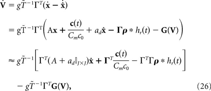where above we again used the fact that x ≈ x̂. Equating this definition of the derivative of V to Equation 24, we find the following:

where Φ = (Γ^T)^†T̃ and (Γ^T)^† = (ΓΓ^T)⁻¹Γ is the Moore-Penrose pseudoinverse of the rectangular matrix Γ^T. Thus, the new dynamics would be as follows:

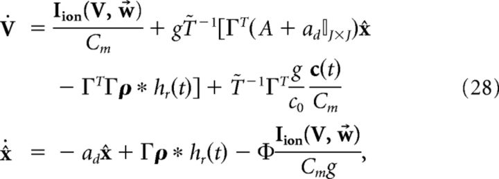which implies that V and x̂ are coupled, as the solution of x̂ is as follows (ignoring initial conditions):

This coupling implies that the decoder x̂ requires instantaneous knowledge of the voltages of each cell. Clearly, a more realistic, and simpler, implementation would be if the decoder had access only to the spike times of the cells. We next show how this can be achieved. We begin with the assumption that the primary cause of the disruption of Equation 23 occurs only during an action potential. We then find an approximation of the intrinsic current I_ion(V, w⃗)/C_m that follows a spike. That is, we seek a kernel η(t) such that:

where t_j^k is the time of the j^th spike of cell k and t_s is the width of the kernel η(t). More details on obtaining the kernel η(t) are provided in the next section. Inserting the above approximation into the last term in Equation 29, we obtain the following:

where η̇(t) = ${\displaystyle {\int }_0^t\eta \left(s\right)e^{-a_d\left(t-s\right)}ds}$. Note that η(t) has units of millivolts per second, whereas η̇(t) has units of millivolts. We can then rewrite the network dynamics as follows:

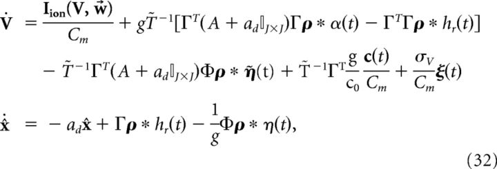where the voltage noise term has again been included. Finally, we introduce the following more compact notation:

where

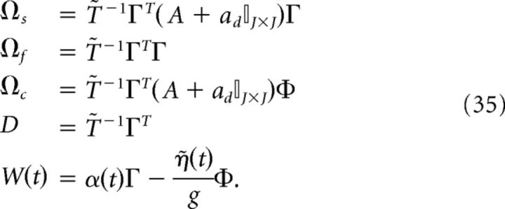We reiterate that the compensation affects both the network dynamics and the readout. Note also that the parameter g scales the strength of the slow and fast synaptic input.

Obtaining the compensation kernels.

The compensation kernel η(t) was obtained by stimulating a single model neuron with a Gaussian noise current (specifically, an Ornstein–Uhlenbeck process; Uhlenbeck and Ornstein, 1930), and keeping track of the times t_j that the voltage crossed a threshold from below. This threshold was the same as that used for detecting spikes in the network simulations. For each spike, we then obtain an action potential waveform V_AP^j(t) for t_j ≤ t < t_j + t_s, where t_s sets the width of the η(t) kernel. We then sum these traces to obtain the average waveform of the action potential V_AP(t). That is, if K spikes were recorded, then:

Thus, an approximation to the change in voltage during the spike is given by the following:

The kernel η(t) is then defined as follows:

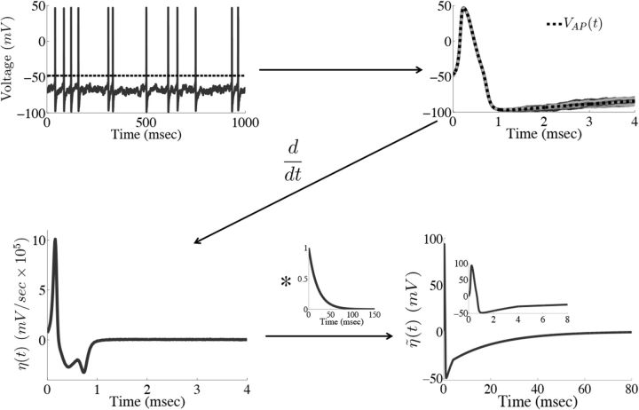
Figure 2 provides an illustration of this procedure. For our simulations, we set t_s = 4 ms. Using a larger value of t_s did not significantly affect the results, but too small a value does, as the voltage trace during the entire time course of the action potential will not be accounted for.

Figure 2.

Obtaining the compensating synaptic kernels. The compensation kernel η(t) was obtained by stimulating a single model neuron with a fluctuating (OU) current and keeping track of the times t_j that the voltage crossed a threshold from below (black dashed line in first panel). For each spike, we then obtain an action potential waveform V_AP^j(t) for t_j ≤ t < t_j + t_s, where t_s will set the width of the η(t) kernel (we take t_s = 4 ms). We then sum these traces to obtain the average waveform of the action potential V_AP(t) (black dashed line in the second panel). The kernel η(t) is then the temporal derivative of this averaged action potential waveform (third panel). η(t) represents an approximation to the total change in voltage of the neuron during an action potential. Last, η(t) is convolved with an exponential function to obtain the synaptic kernel η̃(t) (last panel). Note that η̃(t) changes sign but also very rapidly goes to zero as time goes on. Inset in the last panel shows the η̃ kernel over a shorter period of time.

Decoding variance and approximations.

In this section, we assume that the network tracks a one-dimensional signal; that is, J = 1. The decoder is given by the following:

where ρ^Y = ρ * Y(t), Y ∈ {α, η̇}. The variance of the decoder is then given by the following:

where C_ij^α = cov(ρ_i^α, ρ_j^α), C_ij^η̇ = cov(ρ_i^η̇, ρ_j^η̇), and C_ij^αη̇ = cov(ρ_i^α, ρ_j^η̇). Similarly, the variance of a decoder that assumes that all neurons are independent is given by the following:

where D^X shares the same diagonal elements with C_X but is zero on the off-diagonals and X ∈ {α, η̇, αη̇}.

In the main text we quantify the relative decoding variance of the independent versus “full” (i.e., correlated) network via the fraction ν_x̂^ind/ν_x̂. Values of this fraction greater than one indicate that the network produces correlated spike times that reduce decoding variance versus the “shuffled,” independent case; we refer to it as the “reduction in decoding variance.” To compute this quantity, we performed eight-hundred 2 s runs of the network, with a new noise realization on each trial, calculated the covariance matrices for each trial, averaged the covariance matrices across all trials and used the averaged matrices in Equations 40 and 41.

For the homogeneous network considered below, we can obtain a simple estimate for the reduction in decoding variance. Suppose that Γ_k = a for k = 1,.., N/2 (stimulus-activated population; see main text) and Γ_k = −a for k = N/2 + 1, …, N (stimulus-depressed population; see main text) for some constant a. Then Φ_k = b for k = 1,.., N/2 and Φ_k = −b for k = N/2 + 1,…, N for some constant b related to a. Assume that the variance of each neuron is very close to the average variance over the population, i.e., that the diagonals of each of the above covariance matrices are constant. Dividing each of the above covariance matrices by this average variance σ_X yields a matrix with ones on the diagonal and the various pairwise correlation coefficients on the off-diagonals. Assuming that the pairwise correlation coefficients are close to their average values, the above matrices have a very simple form:

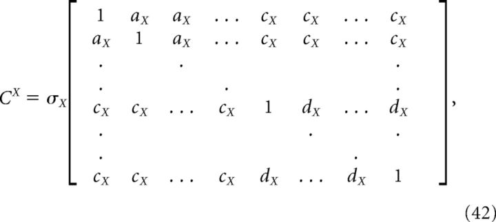where a_X (d_X) is the mean correlation coefficient for the stimulus-activated (stimulus-depressed) population computed using kernel X, and c_X is the mean correlation coefficient between the two different populations using kernel X. With this approximation, the elements of the above variance calculations take a simple form:

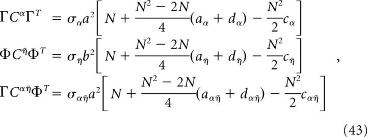and

Thus, an approximation to the reduction in decoding variance obtained by recording from only a subset of the full network is given by using the above formulae in ν_x̂^ind/ν_x̂, because the correlation coefficients do not vary with N. However, if we assume that the dominant contribution to the variance calculation is given by those terms involving the C_α matrix (which is what we find numerically, compare Fig. 11a), then an even simpler formula can be obtained:

Figure 11.

Reduction in decoding variance and error scale with the number of recorded neurons. We explore how the network output varies if we only have access to a subset of neurons in the full-simulated network. The parameters are the same as in Figure 4 and we only show results for the box function input. a, Plots the reduction in decoding variance (see Materials and Methods, Decoding variance and approximations) as a function of the number of simultaneously recorded neurons M. The solid trace shows the results from the numerical simulations while the dashed trace plots the analytical approximation that uses the mean correlation coefficients of the full N = 400 network. b, Plots the square root of the integrated squared error between the estimate and the actual signal as a function of the number of simultaneously recorded neurons on a log-log plot. The dashed trace is the line $1/\sqrt{\text{Number\hspace{0.17em}of\hspace{0.17em}Recorded\hspace{0.17em}Neurons}}$, which would be the prediction of a network of independent Poisson processes. Notice that the error in our network initially decreases like $1/\sqrt{M}$, but eventually begins to decrease at a much faster rate.

Computing correlation coefficients.

The reported correlation coefficients between cells i and j are computed by convolving spike trains with a double-exponential function, so that ρ^α = ρ * α(t):

where T is the total number of time points taken for a given simulation, t_n is the nth time point, and ρ̄^α = T⁻¹∑_n=1^T ρ^α(t_n) is the sample mean. To remove the covariance in firing rates of the cells, the correlation coefficients were corrected by subtracting off the correlation coefficient obtained from shift-predictor data (shifted by one trial). Since our networks consist of two populations of neurons, i.e., those with a positive value for Γ and those with a negative value for Γ, the correlation coefficients reported in the histograms are the population-averaged correlation coefficients for each trial simulation of the network. To generate the histograms, we ran 800 two-second simulations of the network with the same box function input. The only thing that varied between the simulations was the realization of the white background noise.

Computing Fano factors.

The Fano factors for each neuron were computed by binning the spike times into 20 ms windows and computing the mean μ_w and variance σ_w² of the spike count in a particular window over 800 repeated trials of the box function input stimulus. The Fano factor in a particular window is then given by σ_w²/μ_w. For each neuron, the time averaged Fano factor was computed by taking the mean over all windows. We then averaged these values over all neurons in a given population and report them in Figure 5.

Figure 5.

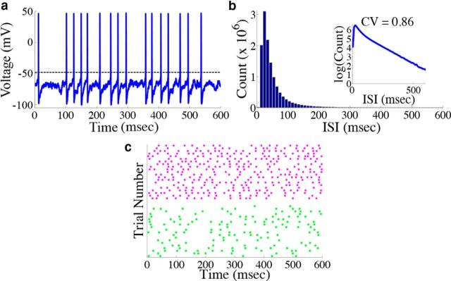
Neurons in the network display irregular spiking. a, Example voltage trace from a single neuron from the homogeneous integrator network with the box function input as in Figure 4. The dashed line represents the threshold used for spike detection. b, Histogram of the interspike intervals of the network during the period of zero stimulus. The inset shows the same data replotted with the y-axis on a log scale. The coefficient of variation in this case is 0.86. c, Raster plot of the spike times of two example neurons (one from each population) on 20 different simulated trials. The magenta (green) dots correspond to the spike times of a neuron from the stimulus activated (stimulus depressed) population. To quantify the trial-to-trial variability, the time averaged Fano factor was computed for each neuron in the network, and then averaged over all cells in each population. This gave 0.515 ± 0.003 for the stimulus-activated population and 0.761 ± 0.002 for the stimulus-depressed population.

Error metrics.

Two measures of error quantify the network performance. The first is the relative error between the signal and the estimate:

where ‖f‖₂ = $\sqrt{{\int }_0^T{\left[f\left(s\right)\right]}^{2}ds}$ and T is the simulation time. Relative error is useful for comparing errors across signals that vary in magnitude. The second error measure is the integrated squared error:

Voltage cross-correlograms and power spectra.

To analyze the subthreshold voltages of cells in our network, we first truncated the membrane potentials at −60 mV to remove the spikes and subtracted out the temporal mean, i.e., V̄_m(t) = V_m(t) − N⁻¹∑_t=1^N V_m(t), where N is the total number of data points. Voltage power spectra for individual neurons were then computed using MATLAB's fft function. Cross-correlations between two cells V̄_m1 and V̄_m2 were also calculated using MATLAB's xcorr function:

where τ is the time lag (Lampl et al., 1999; Yu and Ferster, 2010). We then subtracted off the cross-correlation for shift-predictor data (shifted by one trial). Both the power spectra and cross-correlograms were then averaged over one-thousand 800 ms simulations of the homogeneous integrator network with the box function input.

Computing the spike-triggered error signal.

The spike-triggered error of Figure 5 was computed from eight-hundred 2 s simulations of the network with a box function input (see below). For each simulation, we computed the following:

where e ∈ ℝ^N is the non-dimensional error each neuron is supposed to be representing in its voltage traces. The error e_k(t) was aligned to the spike times for cell k and these traces averaged over all neurons in the network. The shuffled spike-triggered error, computed by aligning e_k(t) to the spike times of cell k on a different trial, was then subtracted. This removed the slow bias present in the original spike-triggered error. Last, the shuffle-corrected spike-triggered errors were averaged over all trials.

Measuring population synchrony.

The level of synchrony in the simulated network was evaluated using a measure introduced by Golomb (2007). With f_k(t) as the instantaneous firing rate of neuron k, synchrony is given by the following:

where 〈…〉_t denotes time-averaging over the length of the simulation. To estimate instantaneous firing rates, the spike trains were convolved with a Gaussian kernel with SD 10 ms.

Scaling when varying the simulated network size.

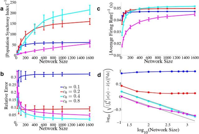
When varying the simulated network size as in Figure 12, we scaled the connection strengths of the network so that the total input to any cell in the network remains constant as the network size is increased. In particular, for the homogeneous integrator (A = 0) network tracking a one-dimensional dynamical system where Γ_k = a for k = 1, 2, …, N/2 and Γ_k = −a for k = N/2 + 1,…, N, we used the scaling:

Thus, both the connection weights and the synaptic gain parameter g scale with 1/N. The factors of 40 and 400 above were chosen so that at N = 400, Γ_k = ± 0.1 and c₀ = g, which matches our earlier simulations of our network when we fixed N at 400. With this scaling, the connection strengths all scale the same way with N and the input c(t) remains constant. To see this, recall that when A = 0 our network equations are given by the following:

where T_k = Γ_k²/2, Φ = (Γ^T)^†T̃, and T̃ is a diagonal matrix with T_k on the diagonal. Thus, we need to determine the scaling of the following:

First, we explore the term Φ which involves the pseudoinverse of the Γ^T matrix. In the case of the homogeneous integrator network, the pseudoinverse is simply given by (Γ^T)_k^† = ± (Na)⁻¹, because (Γ^T)^† Γ^T = 1. Thus, if we let a ∼ 1/N as listed above, (Γ^T)_k^† ∼ 1. Φ_k = [(Γ^T)^†T̃]_k then scales like 1/N². Using this fact, and recalling that g ∼ 1/N, we can now compute the scalings for all the connections in the network:

where we used the fact that since a_d and σ_V are constants, they scale like 1. Thus, the connection weights scale like 1/N. However, because each cell in the network receives input from all N other cells, this scaling means that the total input each cell receives remains constant as the network size is varied.

Figure 12.

Varying the simulated network size. We explore how the network output varies when we change the total number of simulated neurons. We again use the homogeneous network with Γ_k = a for k = 1, 2,…, N/2 and Γ_k = −a for k = N/2 + 1,…, N, σ_V = 0.08 μA/cm² · $\sqrt{s}$, and the box function input. As derived in the Material and Methods, Scaling when varying the simulated network size, we use the scaling a = 40/N, g = c₀(400/N), and the different colored lines correspond to different values for c₀. Error bars represent SDs over 900 repeated trials. a, We plot the inverse of the population synchrony index as a function of the simulated network size for different values of the parameter c₀ which scales the gain of the synaptic input. b, Relative error between the estimate and the actual signal as a function of N. c, The inverse of the time and population averaged firing rate during the period of zero stimulus input as a function of N. d, Square root of the mean integrated error as a function of N on a log–log plot. The two dashed black lines plot 1/$\sqrt{N}$ starting from the first cyan data point and the first magenta data point.

Models and parameters.

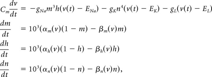
We use a neuron model due to Traub and Miles (1995) and Hoppensteadt and Peskin (2001):

where

and

The factor of 10³ in the gating variable equations comes from conversion of time units from milliseconds to seconds. Other neuron models, including an exponential integrate-and-fire model, were used with similar results.

Other parameters held constant in our simulation are as follows:

The decay rate of a_d = 50 Hz yields a decay time constant of 20 ms for the slow, double-exponential function synapses in our network. This decay time constant is in the range of those observed in inhibitory and excitatory postsynaptic currents (Xiang et al., 1998; Rotaru et al., 2011). The rise rate a_r = 200 Hz sets the decay time scale for the fast, exponential synapses. These synapses have a decay time constant of 5 ms, as observed in inhibitory cells in rat somatosensory cortex (Salin and Prince, 1996).

Simulations.

Simulations were written in MATLAB. The Euler–Maruyama method was used to integrate the stochastic differential equations using a time step of 0.01 ms. Simulations with time steps of 0.005 and 0.02 ms yielded similar results. Spikes were counted as voltage crossings of a threshold of −48 mV from below. The initial voltages for the network were chosen randomly, whereas the channel variables were set to their steady-state values given the fixed initial voltage. In particular, the initial voltages were chosen from a Gaussian distribution with a mean of E_L and a SD of 9 mV. The initial state for the signal and the decoded estimate were both set to zero, i.e., x(0) = x̂(0) = 0.

Though we have provided the most general form for the network tracking any linear dynamical system, throughout the majority of the paper, we focus on the case of a homogeneous network integrating a one-dimensional signal. That is, we set J = 1, A = 0, and Γ_j = a for j = 1,…, N/2 and Γ_j = −a for j = N/2 + 1,…, N, where a is a constant. The only exception to this is in the examples in Figure 1, where we set A = −a_d to remove the slow synapses in the network dynamics. We also set c₀ = g for all figures except Figure 12.

Figure 1.

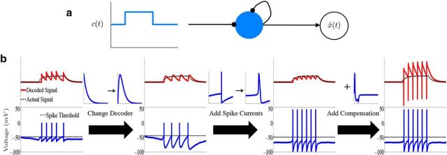
Leaky integration with a single biophysical neuron. a, Diagram illustrating the connectivity of a “network” consisting of a single neuron (N = 1). The diagram shows that the neuron receives stimulus input as well as input from synaptic connections to itself, and the decoder x̂(t) “reads-out” the computation from the spike trains of the network. b, Schematic of how the network is derived in the case of a single neuron. The upper plots show the decoded signal x̂(t) (red traces) plotted against the actual signal x(t) (dashed black lines) along with the neurons' voltage trace (bottom). For the examples in this figure, the network is performing leaky integration on a box function input. In the first column, we illustrate the output of a single neuron from the LIF framework of Boerlin et al. (2013). In the second column, we alter how the stimulus information is read-out from the spike-times of the network (first arrow) which results in an LIF network without instantaneous (δ-function) synaptic dynamics. Going from the second to third columns, we add spike-generating, HH-type ionic currents to the voltage dynamics. The fourth column illustrates how the addition of the compensating synaptic kernel affects the output of the decoder.

We focus on the network integrating one of two different signals. The first varies between two constant values (“box” input):

where t₀ = 100 ms for Figure 4 and t₀ = 0 ms for all subsequent figures. The second is a frozen Ornstein–Uhlenbeck (Uhlenbeck and Ornstein, 1930) signal given by the following:

where ξ(t) is a frozen white noise realization with zero mean and unit variance, τ = 10 ms, and σ = 0.008 μA/cm · s^3/2.

Figure 4.

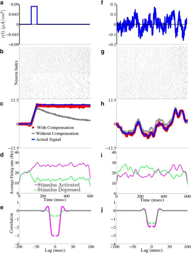
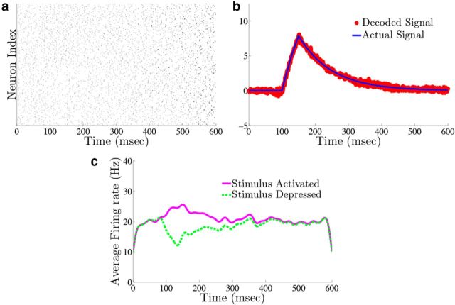
Homogeneous integrator network. We show the output of a network of N = 400 cells where Γ_k = 0.1 for k = 1,…,N/2 (stimulus activated population) and Γ_k = −0.1 for k = N/2 + 1,…, N (stimulus depressed population), g = 0.4 mV, σ_V = 0.08 μA/cm² · $\sqrt{\text{s}}$, and c₀ = g. All other parameters are given in Materials and Methods, Models and parameters. The output of the network with the box function input stimulus are shown in a–e, whereas f–j show the output with the OU stimulus input. a, f, Plot of the stimulus input c(t) into the network. b, g, The raster plots of the 400 cells in the network. The top 200 rows are the stimulus-activated population, whereas the bottom 200 rows are the stimulus-depressed population. c, h, Plot of the network estimate (red) against the actual signal (blue) along with the estimate obtained if compensation was not included (gray). d, i, Plot of the average firing rates for the stimulus activated (magenta) and stimulus depressed (green) populations. e, j, The population averaged autocorrelograms.

Results

Spike-based computation with conductance-based neurons

Our goal in this work is to design a network to carry out an arbitrary linear computation on an input over time, and to do so with neurons that generate spikes via realistic ionic currents and synaptic timescales. Writing the computation as a linear dynamical system, ẋ = Ax + input, where A is a constant matrix and x is the signal we desire to compute; Boerlin et al. (2013) were able to construct a recurrent spiking network to accomplish this goal. The strategy was to arrange connections so that the voltage of each neuron would be proportional to a difference between the currently decoded network output and the ideal computation, trigger spikes when this error exceeds a threshold, and communicate these spikes (and hence the error) to other neurons in the network. Thus, every action potential occurs at a precise time that serves to reduce the “global” computational error across the network. We refer to this framework as spike-based computation.

In this previous work, the authors successfully mapped the requirement of each spike reducing output error onto a network of recurrently connected linear integrate-and-fire neurons with instantaneous synaptic dynamics. However, biological networks have slower synaptic kinetics, and have ionic currents with nonlinear dynamics that determine spike generation. Here, we will show how these two aspects of neurophysiology in fact can fit naturally with spike-based computation.

In particular, we want to design a network of neurons such that an estimate x̂(t) of a J × 1 vector of signal variables x(t) can be linearly read out from the spike times of the network. As above, we assume the signal variables obey a general linear differential equation ẋ = Ax + input. Thus, A is a J × J dimensional matrix and the input is J-dimensional. The entries of the matrix A determine the type of computation the network is asked to perform on the J-dimensional inputs, which we will denote as c(t). For example, if A is the zero matrix, then the network integrates each component of the input over time. Our network will consist of N neurons with output given by the N spike trains, written as ρ_k(t) = ∑_jδ(t − t_j^k) k = 1,…, N.

Our first goal is to incorporate synapses that have finite temporal dynamics. The synaptic dynamics enter through the definition of a decoder that provides an estimate for the variable x. This decoder includes a linear transformation of the network spike trains ρ(t) via a J × N linear decoding matrix Γ. The spike trains ρ_k are first convolved with the synaptic filter α(t) (ρ * α(t) = ∫ ρ(s)α(t − s)ds), which we take to be a standard double-exponential function. With these synaptic dynamics in this decoding, an estimate of the computed variable is given by x̂(t) = Γρ * α(t). The Γ matrix will determine the connectivity structure of the network (see Materials and Methods, Optimal spike-based computation with finite time-scale synapses).

Given this decoder, we now follow (Boerlin et al., 2013) to derive the network dynamics and connectivity. The key step is requiring that neurons in the network only spike to reduce the integrated squared error between the signal and its decoded estimate. As shown in Materials and Methods, this has the consequence that each neuron in the network has a voltage that is equivalent to a weighted error signal, i.e., the voltage of the k^th neuron is given by V_k(t)∝Γ_k^T(x(t) − x̂(t)) (Γ_k^T is the kth column of the N × J matrix Γ^T). Each neuron then fires when its own internal copy of the error signal exceeds a set threshold value. The optimal network that carries out this spike-based computation is given by a network of “pure integrate-and-fire” neuron models that directly integrate synaptic inputs without any leak or intrinsic membrane currents; however, a linear leakage current can be added to the voltage dynamics for each neuron with minimal disruption of the network dynamics (Boerlin et al., 2013). In this case, the voltage dynamics are given by the following:

where −g_L (V − E_L) represents the leakage current. Each neuron receives synaptic input from other cells in the computing network as well as external input. The external input is given by Dc(t), where D is a N × J matrix of input weights, and c(t) is the J × 1 vector of inputs introduced above. The synaptic input is given by gC_mΩ_fρ * h_r(t), where Ω_f is the network connectivity matrix, gC_m scales the strength of the synaptic input, and h_r(t) is a single exponential synapse (see Materials and Methods, Optimal spike-based computation with finite time-scale synapses for details).

Figure 1a illustrates the resulting network structure in the simplest possible case. This is a network consisting of a single neuron that receives stimulus input, as well as input from recurrent (here, autaptic) connections, and a decoder x̂ that reads out the computation from the single neuron's spike train. Figure 1b shows the resulting network behavior. For the examples in this figure, the network performs leaky integration on a single-variable, square wave input (i.e., the matrix A is simply −a_d). The upper plots show the decoded signal x̂(t) from the spiking output of a single neuron (red traces) plotted against the actual desired signal x(t) (dashed black lines) along with the neurons' voltage trace (bottom). In the first column, we illustrate the output of a single neuron from the LIF network of (Boerlin et al., 2013). Comparing the red decoded signal and the actual desired signal x(t) demonstrates the principle of spike-based computation in action: when the decoded signal deviates too far from the desired signal, an additional spike is triggered, and the process repeats.

In the next column, we replace the exponential kernel used for decoding the network spike trains with a double-exponential function (first arrow), as described above, which results in an LIF network without instantaneous (δ-function) synaptic dynamics. Next, as real neurons contain a variety of intrinsic currents, we replace the linear leakage current with generic HH-type ionic currents:

where I_ion(V) represents the sum of all ionic currents and also depends on the corresponding dynamical gating variables. The third column in Figure 1b illustrates how the network behaves with this change to the intrinsic voltage dynamics (labeled as adding “spike currents”).

In general, the addition of such ionic currents to voltage dynamics will disrupt the ability of the network to accurately perform a given computation. This is because the large excursions of the membrane potential during the action potential will cause the voltage of the individual neurons to deviate from their derived optimal relationship with the error. However, in Materials and Methods, Compensating for spike-generating currents, we show that incorporating a new synaptic kernel in both the voltage and decoder dynamics allows the network to effectively compensate for the inclusion of ionic currents, so that it can perform the required computation with improved accuracy compared with the network where these compensation currents are not included. This new synaptic kernel, which we denote by η̃(t), is constructed to counteract the total change in voltage that occurs during a spike. We provide details on how this kernel is derived, as well as how it is obtained for our simulations in Materials and Methods, Compensating for spike-generating currents and Obtaining the compensation kernels, and in Figure 2. The resulting voltage dynamics and decoder are as follows:

where Ω_c is the connectivity matrix for the compensating synaptic connections and W(t) is the new decoding kernel (given in Materials and Method, Compensating for spike-generating currents). The final column of Figure 1b shows how the addition of this compensation current affects the output of a single neuron. For the single neuron case, this adds large fluctuations in the decoder output. Thus, compared with the original effects of adding the spike-generating currents, it appears that the compensation current can decrease accuracy. However, our simulations show that this effect only occurs for very small (<4 neurons) networks. For larger networks, compensation allows the network to perform the computation with a high degree of accuracy, as we will show.

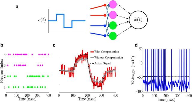
To show how the framework generalizes to larger networks, we plot the output of an example network of N = 4 neurons. For this network, we take Γ_1,2 = a, whereas Γ_3,4 = −a, where a is a constant. The output weights Γ also determine the connectivity structure of the network. This particular choice of Γ will lead to a network with all-to-all connectivity. The matrix D that scales the stimulus input also depends on Γ: the network structure that allows the system to perform accurate spike-based computations requires that D ∝ Γ^T (see Materials and Methods, Optimal spike-based computation with finite time-scale synapses and Compensating for spike-generating currents). This implies that neurons 1 and 2 (3 and 4) will be depolarized (hyperpolarized) when c(t) is positive. The diagram in Figure 3a shows the structure of this network.

Figure 3.

Leaky integration with a network of biophysical neurons. a, Diagram of an example network of N = 4 cells performing leaky integration. In the network, the upper two cells (magenta) are excited by positive stimulus input (indicated by the red lines), whereas the bottom two cells (green) are depressed (indicated by the blue lines). Each neuron receives the stimulus input as well as synaptic input from every other neuron in the network. The spike trains of all four neurons are used in generating the network estimate x̂(t). b, Raster plot from the example network of four neurons. The input to the network in this case is a simple box function, with a fixed positive value from 100 to 200 ms and a fixed negative value from 200 to 300 ms. c, Network estimate x̂(t) (red trace) plotted against the actual signal x(t) (black dashed trace). The gray trace shows the estimate obtained if the compensating kernel was not included in the network dynamics. d, Voltage trace for the topmost neuron in the example network (top row of the raster plot in b).

We next explore the output of our example four-cell network. Here, the input to the network is a simple square-wave function of time, taking a fixed positive value from 100 to 200 ms and a fixed negative value from 200 to 300 ms. Figure 3b shows the resulting spike rasters. The individual spike times are highly irregular, and the upper (lower) two cells appear to be more active when the input is positive (negative). In Figure 3c, we again plot the network estimate x̂(t) (red) against the actual signal x(t) (black dashed). In addition, we also plot what the network estimate would be had the compensating synapses not been included (gray trace). This shows that compensation indeed corrects for systematic biases. Last, Figure 3d plots the voltage trace for an example neuron. There are two key points to take away from this final panel. The first is that the synaptic input is not overwhelming the intrinsic spike-generating currents. Indeed, one way to force the network to behave like an IF network would be to increase the synaptic gain so that the synaptic input is much larger than the intrinsic currents; this is clearly not the case here. The second point to take away from the plot is that the membrane potentials and spike times of individual neurons appear highly irregular.

The above examples, in implementing Equations 58 and 59, used a special choice for the matrix A that defines the linear computation implemented by the network; here, we set A = −a_d so that the connectivity matrix for the double-exponential function synapses is zero (see below and Materials and Methods, Compensating for spike-generating currents). For an arbitrary choice of A, the network dynamics are given by the following:

where Ω_s represents the slow (compared with the exponential fast synapses) synaptic connectivity matrix. This effectively corresponds to the decoded estimate x̂(t) being fed back into the network, which allows the network to perform more general computations on inputs. The parameter g scales the strength of both the slow and fast synapses in the network.

Lastly, in Equation 60 we also added a white noise current (σ_V ξ(t)), drawn independently for each cell, to our voltage evolution equations. This represents random synaptic and channel fluctuations, as well as noisy background inputs, but as we will see below, also serves a functional role in decreasing network synchrony.

Homogeneous integrating network

For the remainder of the paper, we focus on the case of a network of neurons with spike-generating currents based on the Miles–Traub model (Traub and Miles, 1995; Hoppensteadt and Peskin, 2001; Materials and Methods, Models and parameters) which contains HH-type sodium, potassium, and leakage ionic currents. Although we use a specific model, similar results were obtained with different neuron models, e.g., a fast-spiking interneuron model (Erisir et al., 1999) and different sodium, potassium, and leakage current kinetic and biophysical parameters taken from Mainen et al. (1995). We will initially show how such a spiking network can integrate a one-dimensional stimulus input. In terms of the notation previously introduced, this corresponds to the case where the number of inputs, or dimensionality, J = 1 and the matrix A = 0. We choose the input connections such that Γ_k = a for one-half of the cells in the network, k = 1,…, N/2, and Γ_k = −a for the remaining one-half, k = N/2 + 1,…, N. Thus, the network has all-to-all connectivity (recall that the network connectivity matrices depend on Γ, for example, Ω_f ∼ Γ^TΓ); the input to individual neurons within the “first” or “second” half of the network differs only via their (independent) background noise terms. With this configuration, one-half of the network will be depolarized when the stimulus input c(t) is positive, whereas the other one-half will be hyperpolarized. We will refer to the depolarized half as the “stimulus-activated” population and the hyperpolarized half as the “stimulus-depressed” population. Note that this distinction does not refer in any way to excitatory versus inhibitory neurons, as in our formulation neurons can both excite and inhibit one another, a point that we will return to later. The addition of voltage noise in this case is critical as the network is very homogenous and will synchronize in the absence of noise. We systematically explore the dependence of network performance on the noise level (as well as other parameters) in a later section.

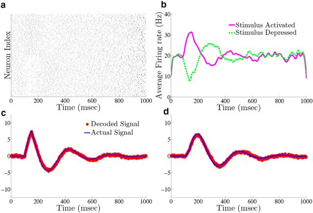
For purposes of illustration, the network was driven with two different types of inputs c(t), a box function and a frozen random trace generated from an Ornstein–Uhlenbeck (OU) process (Uhlenbeck and Ornstein, 1930; Fig. 4a; see Materials Methods for details). The remainder of Figure 4 shows the resulting output for a 400 neuron network, integrating a box input in a–e and integrating the frozen random trace in f–j. Figure 4a and f plot the different inputs, whereas b and g show the raster plots for all 400 neurons. The neurons spike fairly sparsely and highly irregularly. The network estimates, x̂(t) (red trace), along with the true signal x(t) (blue trace) are shown in Figure 4c and h. The network is able to track both the box and OU inputs with a high degree of accuracy: the relative error (Eq. 47), between the estimate and the actual signal is 0.07 for Figure 4c and 0.07 for h. To illustrate the improvement in accuracy due to the synaptic inputs that compensate for spike-generating currents (see Materials and Methods, Compensating for spike-generating currents), we also plot signal estimates from a network where this compensation was not included (gray traces). For these estimates, the relative error is 0.60 in Figure 4c and 0.40 in h; thus, our compensating synapses yield an almost 10-fold increase in accuracy.

Next, we show the population-averaged firing rates for the stimulus-activated (magenta) and stimulus-depressed populations (green) in Figure 4d and i. Figure 4d shows that in the absence of input, the populations maintain persistent activity for ∼500 ms. This is consistent with observations of neural activity during working memory tasks (Jonides et al., 2008). However in Figure 4i, the firing rates of the populations fluctuate depending upon the input. Last, Figure 4e and j plot the average autocorrelation functions for the spiking activity of neurons in the different populations. These display a clear refractory effect, and small tendency to fire in the window that follows. Differences between the stimulus-activated and stimulus-depressed populations, especially for the box function input, are likely due to the different firing rates and inputs that the two populations receive. We explore these spiking statistics further in the section that follows.

Dynamics underlying network computation

We next show that our network displays two key features of cortical networks: the spike times of the network are irregular and Poisson-like, and there is a tight balance between excitation and inhibition for each neuron in the network. Figure 5 shows responses from the homogeneous integrator network introduced in the previous section with a box function input stimulus. The irregularity of spike times is illustrated by the voltage trace of an example neuron in the network, in Figure 5a. To quantify this irregularity, we generated a histogram of the interspike intervals (ISIs) during the period of zero input where the firing rates are nearly constant (Fig. 5b). To generate the histogram, we simulated the response of the network during 800 repetitions of the box function input. The only thing that varied between trials was the realization of the additive background noise current. The ISIs follow an almost exponential distribution, see inset, and the coefficient-of-variation (CV) is 0.86. Thus, the spiking in our network is, by this measure, less variable but not far from what we would expect for Poisson spiking (which would yield a CV = 1) or levels of variability that have been observed in cortical networks (Shadlen and Newsome, 1998; Faisal et al., 2008).

We also explore the trial-to-trial variability of individual neurons in the network. Figure 5c shows a raster plot with the spike times of two example neurons over 20 different trials. The upper (lower) dots correspond to the spike times of a neuron from the stimulus-activated (stimulus-depressed) population. One can see that the spike times of individual neurons vary considerably between trials. To quantify this, we computed the time-averaged Fano factors for each neuron in the network (Materials and Methods, Computing Fano factors). The Fano factor gives a measure of the trial-to-trial variability of individual neurons. For the stimulus-activated population, the time averaged Fano factor, averaged across the population, is 0.515 ± 0.003, whereas for the stimulus-depressed population, it is 0.761 ± 0.002. For a time homogeneous Poisson process, one would expect a Fano factor of 1. Thus, by this measure, neurons in both populations display variable spiking from trial-to-trial, but less variable than what would be expected from a Poisson process.

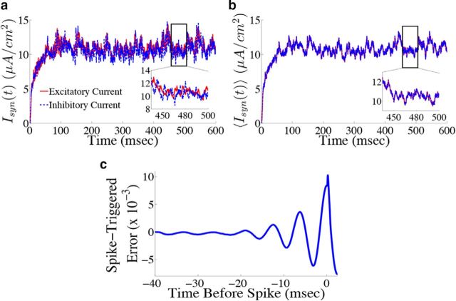
By examining the total excitatory and inhibitory current that each neuron receives, we can check whether the network is in the balanced state (van Vreeswijk and Sompolinsky, 1996; Haider et al., 2006; Okun and Lampl, 2008). To do this, we compute the total positive (negative) input a cell receives. A complication here is that the η̃(t) kernel changes sign; to deal with this, we rewrote the kernel as a difference of two separate, positive kernels, i.e., η̃(t) = η̃_p(t) − η̃_n(t), and computed the resulting current from each kernel. We also ignore the noisy background current for visualization purposes as similar results were obtained when the noise is included. Figure 6a shows the total excitatory (red) and inhibitory (blue) current for an example neuron in the network. Note that although the balance is imperfect (as shown by the inset), the two currents do appear to track each other fairly well. Figure 6b shows the total excitatory (red) and inhibitory (blue) current averaged over all neurons in the network. This shows that the currents are tightly balanced at the level of the entire network, which is typically what one finds when deriving so-called balanced networks (van Vreeswijk and Sompolinsky, 1996; Brunel, 2000; Lim and Goldman, 2013; Ostojic, 2014).

Figure 6.

Neurons in the network display a tight balance between excitation and inhibition, and spike only when the error between the estimated and actual signal is large. a, Total excitatory (red) and inhibitory (blue dashed) currents (ignoring background noise) into an example neuron from the homogeneous integrator network with the box function input as in Figure 4. Inset, A blow-up of a particular time period to show that currents track each other fairly well. b, Total excitatory (red) and inhibitory (blue dashed) currents averaged over all 400 neurons in the network. Inset shows that, on average, the currents are nearly identical, and thus balanced. c, Average projected error signal aligned to the spike times of each neuron in the network, i.e., the spike-triggered error signal (see Materials and Methods, Computing the spike-triggered error signal). The error is largest around the time of a spike indicating that, on average, neurons spike when this projected error signal is large.

Next, we demonstrate that, even after altering the synaptic time scales and including spike-generating currents, neurons in the network still perform predictive coding by firing when their projected error signal is large. We computed the spike-triggered error (STE) for the network by aligning the projected error signal for each neuron k (Γ_k(x(t) − x̂(t)) to that neuron's spike times, averaging across all spike times and then averaging over all neurons (Materials and Methods, Computing the spike-triggered error signal; Fig. 6c). The STE is indeed largest at the time of the spike and rapidly decreases right after the spike, indicating that spikes do in fact decrease the error. The oscillatory behavior of the STE is indicative of the fact that there is some amount of synchrony in the spike times of the network.

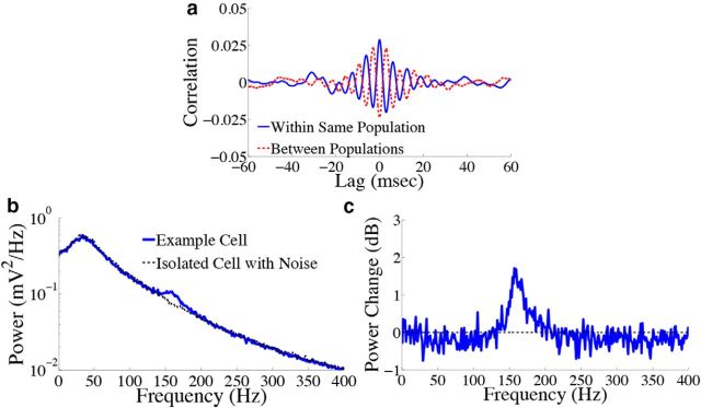
Signatures of spike-based computation are also present in the subthreshold membrane potentials of cells in our network. First, Figure 7a shows the trial-averaged cross-correlogram (see Materials and Methods, Voltage cross-correlograms and power spectra) between the subthreshold voltages of two example cells in the stimulus-depressed population (blue solid trace) and two example cells in different populations (red dashed trace). The voltage traces of cells within the same population appear to be correlated over short time lags, as we expect from the fact that neurons in the same population receive highly similar synaptic input. Meanwhile, voltages of cells in different populations are anti-correlated. Thus, cells in different populations can be differentiated via correlations in their subthreshold voltages. Next, we explore the voltage statistics of single cells. Figure 7b shows the voltage power spectrum of an example cell in the stimulus-depressed population (solid trace). For comparison, the power spectrum of an isolated neuron that only receives background noise input is shown in the dashed trace. It appears that noise input drives the peak in the power spectrum ∼40 Hz, whereas the fast predictive coding implemented by the feedforward input and lateral connections is responsible for the remaining peak ∼150 Hz (Fig. 7c gives a closer view of this second peak). The presence of this second peak is therefore another prediction of the spike-based predictive coding framework.

Figure 7.

Error signal affects the correlation of the subthreshold voltage activity in the homogeneous integrator network with the box function input. a, Trial averaged cross-correlation between the subthreshold voltage activity of two cells in the stimulus-depressed population (blue solid trace) and two cells in different populations (red dashed trace). Cells in the same population (different populations) show correlated (anticorrelated) voltage activity over short time lags. b, Trial averaged voltage power spectrum for an example neuron in the stimulus-depressed population (blue solid trace) and for an isolated cell with only background noise input (dashed trace). c, Change in power (expressed in decibels) that occurs when synaptic connections are included (logarithm base 10 of the solid trace in b divided by the dashed trace). Recurrent inputs contribute to the peak in power ∼150 Hz.

Network creates “good” correlations that reduce decoding variance

We now explore the structure of correlations that emerge among the spikes of different cells in the network, and whether these correlations are beneficial or harmful to the network's encoding of an input that has been integrated over time. Specifically, we ask whether these coordinated spike times increase or decrease the variance of the decoded signal around its mean value. As shown in Materials and Methods, Decoding variance and approximations, the variance of the decoded signal is given by the following:

where C_ij^α = cov(ρ_i^α, ρ_j^α), C_ij^η̇ = cov(ρ_i^η̇, ρ_j^η̇), and C_ij^αη̇ = cov(ρ_i^α, ρ_j^η̇) are the average covariance matrices of the spike trains convolved with the two synaptic kernels, i.e., ρ^Y = ρ * Y(t), Y ∈ {α, η̇}. This quantity measures the variability of the network estimate around its average value; lower values of this variance correspond to highly repeatable network estimates from one trial to the next. If the neurons in our network were independent, then the off-diagonal terms in these covariance matrices would all be zero. Thus, the variance of an independent decoder ν_x̂^ind would have the same form as the above equation, except that the off-diagonal terms of the covariance matrices would be set to zero. The ratio ν_x̂^ind/ν_x̂ measures the reduction in decoding variance caused by the structure of pairwise interactions between neurons in the network. The larger this ratio is, the greater the benefit of pairwise correlations between cells. If the neurons in our network were indeed independent, then this ratio would be 1.

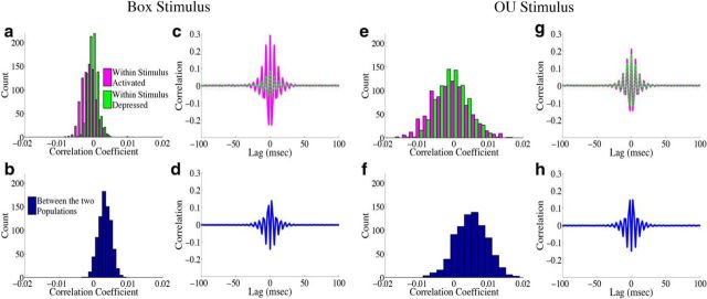
How do correlations affect decoding variance in the homogeneous integrator network? For both of the different inputs, the structure of pairwise interactions between neurons causes an approximately fivefold decrease in the variability of the network estimate: for the box function input, the reduction in decoding variance is 5.0, whereas for the OU input, it is 5.8. To gain insight into how the correlation structure of the network causes this, Figure 8 plots the population-averaged correlation coefficients and cross-correlograms for the homogeneous integrator network. We first focus on the case of the box input function. In Figure 8a we show a histogram of the population-averaged pairwise correlation coefficients for both the stimulus-activated (magenta) and stimulus-depressed (green) populations. Neurons in both populations appear to have weak (and slightly negative) pairwise interactions with one another on average: the mean correlation coefficient for the stimulus-activated (stimulus-depressed) population is −1.3 × 10⁻³ (−0.3 × 10⁻³). On the other hand, Figure 8b shows that the pairwise correlation coefficients between cells in the two different populations are small but positive, with a mean of 3.3 × 10⁻³. Thus, the network reduces decoding variance by creating negative correlations between neurons that represent the same aspect of the stimulus, and positive correlations between neurons that represent different aspects of the stimulus. From a coding perspective, these represent good correlations as the negative correlations between cells in the same population act to reduce redundancy, while the positive correlations across populations allow for some of the background noise to be cancelled out when the estimates from two populations are subtracted (Averbeck et al., 2006; Hu et al., 2014). This can also be seen in the cross-correlograms of the different populations, Figure 8, c and d.

Figure 8.

Structure of spike time correlations for the homogeneous integrator network. The structure of spike time correlations for the network with the box function input are shown in a–d, whereas e–h show the structure of the network with the OU input. a, e, A histogram of the population averaged pairwise correlation coefficient between cells in the stimulus activated population (magenta) and between cells in the stimulus-depressed population (green). In a, the mean correlation coefficient across trials for the stimulus-activated (stimulus-depressed) population is −1.3 × 10⁻³ (−0.3 × 10⁻³), whereas in e it is −1.0 × 10⁻³ (−0.7 × 10⁻³). b, f, A histogram of the average correlation coefficient between cells in the two different populations. In b, the mean correlation coefficient across trials is 3.3 × 10⁻³, whereas in f it is 5.0 × 10⁻³. c, g, Plot of the population and trial averaged shift-predictor-corrected cross correlograms for the raw spike trains of neurons within the stimulus activated (magenta) and stimulus-depressed (green) populations. d, h, Plot of the population and trial averaged shift-predictor-corrected cross correlograms for the raw spike trains of neurons in the two different populations.

The situation is very similar for the OU stimulus input as shown in Figure 8e–h. There are slight differences in that the correlation coefficients are more broadly distributed, Figure 8e, and the correlation structure of the stimulus-activated and stimulus-depressed populations are more similar than for the box function stimulus. This is likely due to the fact that, with the OU stimulus, the two populations receive a more similar range of inputs over time.

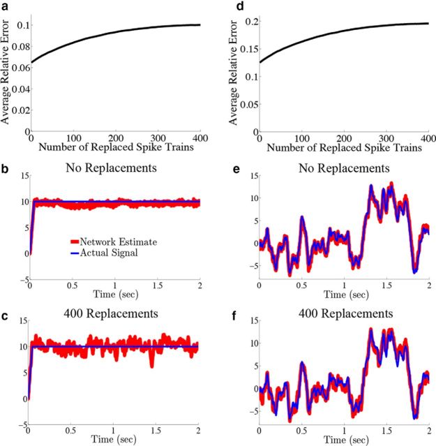
We have shown that the structure of pairwise interactions between neurons in the network acts to greatly reduce the variability of the network estimate of the underlying computation on a stimulus input. This already reveals a difference between this framework and the underlying assumptions of a rate model, in which neurons in the network are assumed to be statistically independent. As such, one could shuffle the spiking output of individual neurons from different trials and the rate-based computation would suffer no loss in accuracy. However, for the predictive coding network, it was shown that the structure of interactions between spike trains for individual neurons from trial to trial is important to the accuracy of the desired computation (Boerlin et al., 2013). To give a more direct illustration of this effect with our current network, we explored how the relative error between the decoded network estimate and the actual signal varied as we replaced an increasing number of spike trains with variations recorded from separate trials (“shuffled” trains).

Figure 9a plots the average relative error between desired (x) and network-decoded (x̂(t)) signals (see Materials and Methods, Error metrics) as a function of the number of shuffled spike trains, for the box function input. As expected, the error increases with the number of shuffled trains and reaches its maximum when all spike trains are taken from separate trials. To see how the shuffling affects the network estimate, we show an example decoded estimate (red) plotted against the true signal (blue) in Figure 9b when all spike trains are taken from the same trial. In Figure 9c, we plot the estimate decoded from entirely shuffled spike trains, where all are taken from different trials. As also expected from the previous section, the effect of shuffling spike trains appears to increase the magnitude of the fluctuations of the decoded estimate around its mean value. Figure 9d–f show that the situation is similar with the OU stimulus, although it is more difficult to see the effects on the decoded signal due to the fluctuations in the OU signal itself.

Figure 9.

Shuffling spike trains across trials distinguishes the network from a rate model. We explore how the decoding error varies as we decode the spiking output of the network where we replace an increasing number of individual neuron spike trains with those from different trial simulations. The parameters are the same as those used in Figure 4. a, Plots of the relative error (Eq. 47) as a function of the number of replaced spike trains for the network with the box function input. As the number of replaced spike trains is increased, so does the error. b, Plots an example network estimate (red) against the actual signal (blue) when no spike trains have been replaced. c, Plots the network estimate (red) against the actual signal (blue) when all 400 spike trains are taken from separate trials. Notice how replacing spike trains increases the variability of the estimate around its mean. For comparison, the relative error in b is 0.05, whereas in c it is 0.09. d–f, The same as a–c except that the OU stimulus is used. The relative error in e is 0.09, whereas in f it is 0.18.

Sensitivity to variation in synaptic strength and noise levels

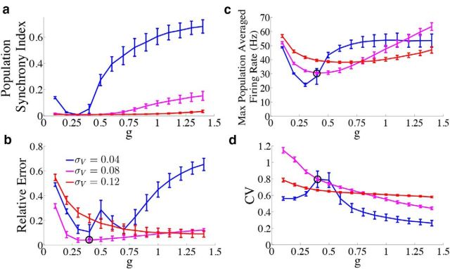
Our previous examples of the behavior of the homogeneous integrator system made use of a particular choice of network parameters. We now explore the sensitivity of its performance to changes in these parameters. In particular, we vary the strength of the fast and slow synaptic input, g, and the strength of the added voltage noise, σ_V. For the homogeneous integrator network, these two parameters have the largest effect on performance as g effectively scales the strength of synaptic connectivity between neurons in the network and σ_V creates a level of heterogeneity in the individual voltage dynamics that prevents cells from synchronizing. We will show that the performance of our network is fairly robust to changes in these parameters.

We quantify network behavior using several measures. As before, the accuracy of the computation is evaluated using the relative error between the network estimate and the true signal. To assess the firing properties of the network, we compute a population synchrony index introduced by (Golomb, 2007; see Materials and Methods, Measuring population synchrony), and the coefficient of variation of the interspike intervals during periods of zero stimulus input (for the box function input). We also track the maximum population-averaged firing rate, to ensure that the populations are not firing at unrealistically high levels. Because similar results were obtained with the OU stimulus, we only report these metrics for the box function stimulus.

We first investigate how the level of population synchrony interacts with the accuracy of the network and neuronal firing rates. Figure 10a plots the population synchrony index as a function of the synaptic gain g for three different values of the noise strength. The population synchrony has a U-shaped dependence on g; this is easiest to see at the smallest noise level. When the population synchrony is high, the relative error is large (Fig. 10b) and firing rates approach unrealistic levels (Fig. 10c). Thus, desynchronizing the firing dynamics of individual neurons in the network by increasing the noise to moderate levels improves network accuracy. Our interpretation is that moderate noise distributes the computation more efficiently among individual neurons. If the noise is too small, then individual neurons behave too similarly and eventually synchronize, effectively reducing the dimensionality of the network and also the computational power. When the noise is too large, the computation is overpowered by the noise.

Figure 10.

Dependence of network statistics on noise and synaptic gain parameters. We explore how the network output changes as we vary the synaptic gain parameter g and the strength of the voltage noise σ_V. We set the parameter c₀ which scales the strength of the input to c₀ = g for every value of g used. Because the results were similar for the frozen noise (OU) case, we only plot the results for the network with the box function input. b–d, We indicate the parameter values used in the previous figures with a black circle. Error bars represent SDs over 300 trials. a, Population synchrony index (see Materials and Methods, Measuring population synchrony) as a function of g for three different noise levels σ_V = 0.04 μA/cm² · $\sqrt{s}$ (blue trace), σ_V = 0.08 μA/cm² · $\sqrt{s}$ (magenta trace), and σ_V = 0.12 μA/cm² · $\sqrt{s}$ (red trace). b, Relative error between the estimate and the actual signal as a function of g. c, Maximum population averaged firing rate as a function of g. d, Coefficient of variation of the ISIs during the period of zero stimulus input as a function of g.

Figure 10b plots the relative error between the network estimate and the true signal as a function of g for three different noise levels. As in Figure 10a, for the first two noise levels (blue and magenta traces), the error appears to display an almost U-shaped dependence on g, indicating that there is an optimal choice for g that minimizes the error for each noise level. This value of g also corresponds to the lowest value of the population synchrony index. However, for the largest noise level (red trace), the error monotonically decreases as g is increased. This could be indicative of the fact that, for this noise level, the population remains fairly desynchronized for a wide range of g values. The effects of increasing the noise also depend on the value of g. For small g, increasing the noise level first acts to decrease the error (compare blue to magenta), but then drives it to its highest level (red trace). However, when g is larger, noise appears to always cause the error to decrease. For reference, the black circle on the magenta trace shows the values of g and σ_V that were used in the previous sections.

How do these parameter choices affect the networks' firing rates? Like the relative error traces in Figure 10b, the maximum population-averaged firing rates (Fig. 10c) also display a U-shaped dependence on g, and the shallowness of the U increases as the noise level is increased. This indicates that with increasing noise, there is a larger range of g values that lead to low firing rates. Last, Figure 10d plots the CV of the ISIs of the network during the period of zero stimulus input. For moderate noise and moderate g, the network maintains CV on the order of 0.8.

In conclusion, network performance is not highly sensitive to changes in synaptic strength g or to the level of added voltage noise, as there exist many combinations of choices that lead to similar network performance.

Recording from a subset of neurons

Until now, we have assumed that the decoder has access to all neurons in the network that is performing the computation on the input; that is, we have fixed our network size at N = 400 cells and have examined its performance using the spiking output of all 400 cells. However, when recording from real neural circuits, it is more likely that one would be measuring from a subset of cells involved in a given computation. The same is possible for different circuits “downstream” of a computing network. We explore how the reduction in decoding variance and the decoding error scales with the number of simultaneously recorded neurons.

Figure 11a plots the reduction in decoding variance ν_x̂^ind/ν_x̂ as a function of the number of simultaneously recorded neurons M for the homogeneous integrator network with the box function input stimulus. The simulated network size was fixed at N = 400. To compute the reduction in decoding variance for a smaller network of size M, a random subset of M spike trains was chosen from a single simulated trial of the full network. We then computed the necessary covariance matrices using these spike trains, and averaged these matrices over all 800 trials. These averaged covariance matrices were used to compute the ratio ν_x̂^ind/ν_x̂ according to the formulae given in Materials and Methods, Decoding variance and approximations. The solid trace in Figure 11a plots the result of these numerical simulations whereas the dashed trace plots the approximation given in Equation 45, which uses the correlation coefficients that were computed using all N cells in the simulated network.

Figure 11b plots the square root of the decoding error (Eq. 48) as a function of the number of simultaneously recorded neurons. As the number of recorded neurons increases, the decoding error initially decreases as $1/\sqrt{\text{Number\hspace{0.17em}of\hspace{0.17em}Recorded\hspace{0.17em}Neurons}}$ (black dashed line), similar to what one would expect for independent Poisson spiking, as implicitly assumed in many rate models. However, as the number of recorded neurons is increased further, the error from the spiking network decreases faster than $1/\sqrt{\text{Number\hspace{0.17em}of\hspace{0.17em}Recorded\hspace{0.17em}Neurons}}$.

The predictions of our network about how the reduction in decoding variance and the decoding error both scale with the number of simultaneously recorded neurons could in principle be tested with dense multielectrode arrays or optical imaging. However, these predictions would have to be modified to incorporate the effects of shared sensory noise or noise in the output of the decoder.

Varying network size

We now explore how the total number of neurons in the network, N, affects the fidelity of the computation. We limit our analysis to integration of the box function stimulus. As derived in Materials and Methods, Scaling when varying the simulated network size, we scale both the entries of the matrix Γ and the synaptic gain parameter g with 1/N. Using this scaling allows the total input to each neuron in the network to remain constant as the network size is varied.

Figure 12 shows the results of these simulations. In particular, we explore how the population synchrony index, the relative error, the time- and population-averaged firing rate, and the integrated error vary as the network size is increased. In all plots, the cyan trace at N = 400 corresponds to the parameters used in our previous network simulations. Figure 12a plots the inverse of the synchrony index as a function of N for four different values of the parameter c₀, which scales the synaptic gain (that is, g ∼ c₀/N). This highlights the differences between the curves corresponding to the different values of c₀. It is clear that synchrony tends to always decrease as the network size is increased, though the maximum level of synchrony reached as well as the rate at which it decreases with N are both affected by c₀. Thus, as we have seen previously in Figure 10, increasing the synaptic gain can lead to increased population synchrony (compare the cyan and magenta traces). Figure 12b plots the relative error as a function of N. For small values of c₀, the error initially increases with N, but quickly reaches an asymptote and remains constant with further increases in network size (blue trace). As c₀ is increased, we quickly see a transition in the curves as the relative error now begins to decrease with N. Increasing c₀ initially causes the error to drop off faster with N (compare the red and cyan traces), but too large of a value for c₀ cause the error to drop off more slowly with N (compare the cyan and magenta traces). Figure 12c plots the inverse time- and population-averaged firing rate during the period of zero stimulus input as a function of N. As with the population synchrony index, the firing rates tend to decrease as N is increased.

In sum, Figure 12a–c illustrate that the computational error produced by the network, as well as its firing rates and synchrony, all tend to decrease for larger networks. We next compare the trend in error against what would be naively expected in a simple “rate network”; that is, one in which each neuron fires according to a prescribed firing rate in a population, and does so with independent Poisson statistics. In this case, we expect that the square root of the mean integrated squared error will scale like 1/$\sqrt{N}$. To compare the error in our spiking network, we plot the square root of the mean integrated squared error as a function of N in Figure 12d. For c₀ = 0.4 (cyan trace), the error decreases as 1/$\sqrt{N}$ (black dashed line) just as for the Poisson rate network. However, for such rate networks, the firing rates of individual units are fixed and do not vary with the network size. In our network, we clearly see a dramatic decrease in firing rates as network size grows, up to ∼N = 400 cells (Fig. 12c). Further increases in network size past this point lead to minimal decreases in the firing rates. The fact that the firing rates for our network change with network size is a strong difference from a Poisson rate network. Thus, even though our network produces a similar error scaling with N as predicted under basic assumptions for firing rate networks, for network sizes between 100 and 400 neurons, it manages to do so in a more efficient manner; it produces the same error with a lower average firing rate (i.e., fewer spikes).

Beyond pure integration: leaky integration and damped harmonic oscillations

In this section, we highlight the generality of our approach by showing the output of the spike-based predictive coding networks that are performing computations other than “pure” integration of its inputs over time. First, we study leaky integration, obtained in Equation 1 by choosing A to be negative (and continuing to take J = 1 dimension for the signal x(t)). Figure 13 shows an example of the network performing leaky integration (A = −10) on the same box function input from Figure 4a. All other network parameters are the same as in Figure 4. The raster plot in Figure 13a shows that the network still displays sparse irregular spiking when performing leaky integration. Figure 13b shows the network estimate (red) plotted along with the actual signal (blue), demonstrating that the leaky integration computation is performed with a high degree of accuracy (the relative error is 0.08). Last, Figure 13c shows the firing rates of both the stimulus-activated and stimulus-depressed populations; note that these eventually return to their baseline (pre-input) levels because the computation is leaky.

Figure 13.

Leaky integration in the homogeneous network. We show the results of the network performing leaky integration on the box function input. All parameters are the same as in Figure 4 except that A = −10; c(t) is the same box function from Figure 4a. a, The raster plot of the 400 cells in the network. The top 200 rows are the stimulus-activated population, whereas the bottom 200 rows are the stimulus-depressed population. b, Plots the network estimate (red) against the actual signal (blue). c, Plots the average firing rates for the stimulus-activated (magenta) and stimulus-depressed (green) populations.

Next, we consider the computation of processing inputs through a two dimensional dynamical system that displays damped harmonic oscillations. Here, the matrix A is chosen as

In this case, the eigenvalues of the matrix A are μ ± iω, and the solutions x(t) of the linear system (Eq. 1) will display damped oscillations as long as μ < 0 (we use μ = −5 and ω = 20). We take Γ to be a 2 × N matrix whose elements are chosen randomly. Last, we use as our input c(t) a vector with c₁(t) being the box function input from Figure 4a and c₂(t) = 0.

Figure 14 plots the resulting network behavior. We again see sparse irregular spiking with firing rates that eventually return to their baseline level (Fig. 14a and b. As the signal x(t) is two dimensional, the network estimate x̂(t) is also two dimensional, and we plot both of the network estimates (red) along with the actual signals (blue) in Figure 14c and d. Once again, the network is able to perform the required computation with a high degree of accuracy (the relative error in Fig, 14c is 0.14 and d is 0.12).

Figure 14.

Damped harmonic oscillations. We show the results of the network processing the box function input via damped harmonic oscillations. All parameters are the same as in Figure 4 except that Γ is now a 2 × N matrix and c(t) is a vector with c₁(t) being the same box function from Figure 4a and c₂(t) = 0. The elements of Γ are chosen randomly with Γ_ij ∈ Unif(0.002, 1) for i = 1, 2 and j = 1,2,…,N/2 and Γ_ij ∈ Unif(− 1, − 0.002) for i = 1, 2 and j = N/2 + 1,…,N. Also, the columns of Γ are normalized so that ‖Γ‖_j = $\sqrt{{\Gamma }_{1j}^2+{\Gamma }_{2j}^2}$ = 0.06. a, The raster plot of the 400 cells in the network. The top 200 rows are the stimulus-activated population, whereas the bottom 200 rows are the stimulus-depressed population. b, Plots the average firing rates for the stimulus-activated (magenta) and stimulus-depressed (green) populations. c, d, Plots of the network estimates (red) against the actual signals (blue).

Discussion

Synaptic kinetics that support spike-based computation

We have shown that networks of neurons with voltage-dependent spike-generating currents and realistic synaptic timescales can perform accurate spike-based computations. These networks are derived based upon the premise that the voltage traces of individual neurons represent an error signal between the network estimate and the actual signal, and that spikes occur whenever the error becomes too large. The key innovation we present that allows the network to accurately perform these computations is the inclusion of synapses with appropriate kinetics. Two factors determine these kinetics. We begin by assuming that signals are “decoded” from the network with synapses that have finite timescales of rise and decay (“double-exponential” synapses). Next, we account for the nonlinear dynamics of spike generating currents with “compensating” synapses, which allow the system to represent the projected error signal in the voltage traces of individual neurons. It is important to note two limitations of these additional factors. The first is that if the rate of rise of the double-exponential synapse is slower than the rate of change of the signal, then the accuracy of the computation will be affected. This is the case because the network simply cannot respond quickly enough to accurately track the signal. Second, the “compensating” synapses we introduce were designed to compensate for currents acting on the timescale of a single action potential. Thus, slow adaptation currents are not accounted for by our approach. This will make it difficult for the network to maintain the persistent activity that is required when the desired computation is pure integration. Interestingly, however, we find that when the desired computation is leaky, simulations suggest that adaptation may have a minimal effect on the performance of the network. Thus, a network with strong adaptive currents is perhaps better suited to implement leaky integration or fast dynamics rather than perfect integration.

Our results prove the principle that mechanisms of spike-based computation previously derived for networks of idealized neurons and synapses (Boerlin and Denéve, 2011; Boerlin et al., 2013) can be extended to settings closer to the underlying biophysics. However, there is still distance to travel before we arrive at a “realistic” biologically based system. The compensating synapses are somewhat complicated functions of time. Moreover, these and other synaptic connections provide both positive and negative currents following a spike, a clear violation of Dale's rule (although recently neurons that release both GABA and glutamate have been found in rodents; Root et al., 2014). More complex synaptic waveforms, and ones that change sign, could be implemented via intermediate synapses with different kinetics (for example, a pathway with delayed feedforward inhibition will produce first positive, then negative, synaptic current). Furthermore, recent advances in learning temporal connections between neurons (Kennedy et al., 2014), together with learning algorithms for the present spike-based computation framework (Bourdoukan et al., 2012), provide a basis to potentially derive a learning rule for the compensation filters. However, a question for future work is whether there are other network configurations that perform spike-based computation without the need for intermediate connections (as for simpler settings by Boerlin et al., 2013), and additionally with simpler synaptic waveforms than the compensating ones derived here.

Computing with spikes and computing with rates

As shown by Boerlin and Denéve (2011) and Boerlin et al. (2013), our network approaches the notion of computations in neural circuits from the standpoint that a computation is distributed among the spike times of individual neurons. This stands in contrast to many studies in which the computation is assumed to be carried at the level of averaged firing rates (Brunel, 2000; Compte et al., 2000; Goldman et al., 2003; Renart et al., 2004; Wong and Wang, 2006; Ostojic, 2014), and to other related studies that derive network dynamics that minimize squared error in signal representation (Rozell et al., 2008). Demonstrating the importance of spike timing in our network, we compared the accuracy of the underlying computation before and after shuffling these times but preserving trial-averaged firing rates (Fig. 9). Shuffling indeed reduced the accuracy, a fact we related to the structure of spike-time correlations produced by the network.

What are the advantages of using such a precise temporal representation? It could be that distributing a computation among the spike times of individual cells endows the network with robustness to perturbations such as synaptic failure and lesions (as was demonstrated by Boerlin et al., 2013). Moreover, a computation performed on the level of spike times opens the possibility that the underlying network structure could be learned via spike-based plasticity rules, as suggested by recent work (Bourdoukan et al., 2012).

Finally, a precise temporal code may leverage the computational power of individual spiking neurons in a more efficient manner than rate-based approaches. Traditional spiking network implementations of rate-based networks employ large amounts of added voltage noise to avoid synchrony, and large cell populations, so that the resulting population output is well described by “mean field” rate equations (Brunel, 2000; Compte et al., 2000; Renart et al., 2004; Machens et al., 2005; Wong and Wang, 2006; Ostojic, 2014). Thus, large populations of cells with noise-driven spiking represent signals in traditional rate-based approaches. The possibility that spike-based computation might give rise to a significantly lower total error for a given population size. This seems likely, given the results by Boerlin et al. (2013), and in our Results, Recording from a subset of neurons. That is, the error in our networks can decrease faster than expected for a population of cells with independent spike times. Making a more direct comparison to rate-based networks is an interesting area for future work.

This said, this spike-based approach to computation is not immune to problems with synchrony, and the need for additive noise to combat it. We showed that there is an optimal level of this noise at which the network retains characteristics of spike-based computation. Moreover, in the current work, we have used a very homogeneous population in which all neurons have the same spike-generating currents and magnitude of synaptic connectivity. Preliminary simulations suggest that more heterogeneous networks better avoid synchrony, and hence may be able to perform computations with higher accuracy.

Balanced networks and irregular spiking behavior

Cortical neurons are known to display irregular Poisson-like firing (Softky and Koch, 1993; Shadlen and Newsome, 1998). What might be the basis of the observed irregularity? Various authors have proposed that the variability is a result of a tight balance between the total excitatory and inhibitory current each neuron in the network receives (van Vreeswijk and Sompolinsky, 1996; Renart et al., 2010). Indeed cortical networks have been shown to display such a balance between excitation and inhibition (Wehr and Zador, 2003; Haider et al., 2006; Okun and Lampl, 2008).

Although successful in reproducing the Poisson-like firing of cortical neurons, it has only very recently been shown that balanced networks can be used to perform particular computations, including integration of inputs over time (Boerlin et al., 2013; Lim and Goldman, 2013). Our work contributes further results in this direction. In contrast to much previous modeling work on balanced networks, the specific condition for balancing excitation and inhibition is not built into the derivation of spike-based computation. Rather, the balanced state arises naturally as a consequence of optimizing the computation at the level of single cells; that is, assuming that neurons represent a projected error signal in their voltage traces and spike when this error becomes too large (Boerlin et al., 2013). Furthermore, our network maintains this balanced state with a relatively small number of cells (Figs. 4, 5). Thus, our work suggests that a computational unit in the brain may require dramatically fewer neurons than predicted by rate-based approaches (Brunel, 2000; Lim and Goldman, 2013; Ostojic, 2014).

Finally, nearly all modeling work on balanced networks makes use of simplified integrate-and-fire neuronal spiking dynamics. Thus, it has remained unclear whether or not the balanced state can be maintained by a network of neurons with more complex spike-generating dynamics. We have shown here that it is indeed possible for a network of such neurons to display a tight balance between excitation and inhibition, and thus display irregular spiking.

Even during a single trial, the neurons in our network display variable spiking behavior. This can be seen from the population firing rates in Figure 4d. Even though the network maintains a constant decoded signal, the average firing rates fluctuate, indicating that not all neurons are displaying the same firing rate. This phenomenon of variable neuronal activity underlying stable network stimulus representation is known to occur (Buzsáki and Draguhn, 2004; Haider and McCormick, 2009; Tchumatchenko et al., 2011) and has recently been shown in a rate model network with a specific architecture (Druckmann and Chklovskii, 2012). Here, we show that stable stimulus representation with variable neuronal responses arises as a natural feature of networks that perform spike-based computation.

Sensitivity and tuning

The performance of network models that integrate inputs over time is typically quite sensitive to the choice of connection weights between neural populations (Seung et al., 2000). If the recurrent connections are either too strong or too weak, the activity of the network can either quickly increase to saturation or decrease to a baseline level. Recent work by Lim and Goldman (2013, 2014) has shown that this sensitivity issue can be resolved in a rate-based network where inhibition and excitation are balanced. In particular, Lim and Goldman show that a balanced rate-based network of LIF neurons can robustly maintain information for working memory with irregular spiking. Further work will be needed to assess whether the spike-based networks derived here have similar robustness to changes in network connection strengths; our preliminary studies suggest that they may not, as perturbing the network structure away from the optimally derived connectivity will lead to decreased network accuracy. However, there is evidence to suggest that the optimal connectivity structure could potentially be learned, and maintained, by plasticity rules (Bourdoukan et al., 2012; Kennedy et al., 2014).

References

- Averbeck BB, Latham PE, Pouget A. Neural correlations, population coding and computation. Nat Rev Neurosci. 2006;7:358–366. doi: 10.1038/nrn1888. [DOI] [PubMed] [Google Scholar]
- Boerlin M, Denève S. Spike-based population coding and working memory. PLoS Comput Biol. 2011;7:e1001080. doi: 10.1371/journal.pcbi.1001080. [DOI] [PMC free article] [PubMed] [Google Scholar]
- Boerlin M, Machens CK, Denève S. Predictive coding of dynamical variables in balanced spiking networks. PLoS Comput Biol. 2013;9:e1003258. doi: 10.1371/journal.pcbi.1003258. [DOI] [PMC free article] [PubMed] [Google Scholar]
- Bogacz R, Brown E, Moehlis J, Hu P, Holmes P, Cohen JD. The physics of optimal decision making: a formal analysis of models of performance in two alternative forced choice tasks. Psychol Rev. 2006;113:700–765. doi: 10.1037/0033-295X.113.4.700. [DOI] [PubMed] [Google Scholar]
- Bourdoukan R, Barrett D, Machens C, Denéve S. Learning optimal spike-based representations. In: Bartlett P, Pereira FCN, Burges CJC, Bottou L, Weinberger KQ, editors. Advances in neural information processing systems. Vol 25. Cambridge, MA: MIT; 2012. pp. 2294–2302. [Google Scholar]
- Brody CD, Romo R, Kepecs A. Basic mechanisms for graded persistent activity: discrete attractors, continuous attractors, and dynamic representations. Curr Opin Neurobiol. 2003;13:204–211. doi: 10.1016/S0959-4388(03)00050-3. [DOI] [PubMed] [Google Scholar]
- Brunel N. Dynamics of sparsely connected networks of excitatory and inhibitory spiking neurons. J Comput Neurosci. 2000;8:183–208. doi: 10.1023/A:1008925309027. [DOI] [PubMed] [Google Scholar]
- Buzsáki G, Draguhn A. Neuronal oscillations in cortical networks. Science. 2004;304:1926–1929. doi: 10.1126/science.1099745. [DOI] [PubMed] [Google Scholar]
- Cain N, Shea-Brown E. Computational models of decision making: integration, stability, and noise. Curr Opin Neurobiol. 2012;22:1047–1053. doi: 10.1016/j.conb.2012.04.013. [DOI] [PubMed] [Google Scholar]
- Compte A, Brunel N, Goldman-Rakic PS, Wang XJ. Synaptic mechanisms and network dynamics underlying spatial working memory in a cortical network model. Cereb Cortex. 2000;10:910–923. doi: 10.1093/cercor/10.9.910. [DOI] [PubMed] [Google Scholar]
- Druckmann S, Chklovskii DB. Neuronal circuits underlying persistent representations despite time varying activity. Curr Biol. 2012;22:2095–2103. doi: 10.1016/j.cub.2012.08.058. [DOI] [PMC free article] [PubMed] [Google Scholar]
- Eckhoff P, Wong-Lin K, Holmes P. Dimension reduction and dynamics of a spiking neural network model for decision making under neuromodulation. SIADS. 2011;10:148–188. doi: 10.1137/090770096. [DOI] [PMC free article] [PubMed] [Google Scholar]
- Erisir A, Lau D, Rudy B, Leonard CS. Function of specific k+ channels in sustained high-frequency firing of fast-spiking neocortical interneurons. J Neurophysiol. 1999;82:2476–2489. doi: 10.1152/jn.1999.82.5.2476. [DOI] [PubMed] [Google Scholar]
- Faisal AA, Selen LP, Wolpert DM. Noise in the nervous system. Nat Rev Neurosci. 2008;9:292–303. doi: 10.1038/nrn2258. [DOI] [PMC free article] [PubMed] [Google Scholar]
- Gold JI, Shadlen MN. The neural basis of decision making. Annu Rev Neurosci. 2007;30:535–574. doi: 10.1146/annurev.neuro.29.051605.113038. [DOI] [PubMed] [Google Scholar]
- Goldman MS. Memory without feedback in a neural network. Neuron. 2009;61:621–634. doi: 10.1016/j.neuron.2008.12.012. [DOI] [PMC free article] [PubMed] [Google Scholar]
- Goldman MS, Levine JH, Major G, Tank DW, Seung HS. Robust persistent neural activity in a model integrator with multiple hysteretic dendrites per neuron. Cereb Cortex. 2003;13:1185–1195. doi: 10.1093/cercor/bhg095. [DOI] [PubMed] [Google Scholar]
- Golomb D. Neural synchrony measures. Scholarpedia. 2007;2:1347. doi: 10.4249/scholarpedia.1347. [DOI] [Google Scholar]
- Haider B, McCormick DA. Rapid neocortical dynamics: cellular and network mechanisms. Neuron. 2009;62:171–189. doi: 10.1016/j.neuron.2009.04.008. [DOI] [PMC free article] [PubMed] [Google Scholar]
- Haider B, Duque A, Hasenstaub AR, McCormick DA. Neocortical network activity in vivo is generated through a dynamic balance of excitation and inhibition. J Neurosci. 2006;26:4535–4545. doi: 10.1523/JNEUROSCI.5297-05.2006. [DOI] [PMC free article] [PubMed] [Google Scholar]
- Hodgkin AL, Huxley AF. A quantitative description of membrane current and its application to conduction and excitation in nerve. J Physiol. 1952;117:500–544. doi: 10.1113/jphysiol.1952.sp004764. [DOI] [PMC free article] [PubMed] [Google Scholar]
- Hoppensteadt FC, Peskin C. Modeling and simulation in medicine and the life sciences. Ed 2. New York: Springer; 2001. [Google Scholar]
- Hu Y, Zylberberg J, Shea-Brown E. The sign rule and beyond: boundary effects, flexibility, and noise correlations in neural population codes. PLoS Comput Biol. 2014;10:e1003469. doi: 10.1371/journal.pcbi.1003469. [DOI] [PMC free article] [PubMed] [Google Scholar]
- Jonides J, Lewis RL, Nee DE, Lustig CA, Berman MG, Moore KS. The mind and brain of short-term memory. Annu Rev Psychol. 2008;59:193–224. doi: 10.1146/annurev.psych.59.103006.093615. [DOI] [PMC free article] [PubMed] [Google Scholar]
- Kennedy A, Wayne G, Kaifosh P, Alviña K, Abbott LF, Sawtell NB. A temporal basis for predicting the sensory consequences of motor commands in an electric fish. Nat Neurosci. 2014;17:416–422. doi: 10.1038/nn.3650. [DOI] [PMC free article] [PubMed] [Google Scholar]
- Lampl I, Reichova I, Ferster D. Synchronous membrane potential fluctuations in neurons of the cat visual cortex. Neuron. 1999;22:361–374. doi: 10.1016/S0896-6273(00)81096-X. [DOI] [PubMed] [Google Scholar]
- Lim S, Goldman MS. Balanced cortical microcircuitry for maintaining information in working memory. Nat Neurosci. 2013;16:1306–1314. doi: 10.1038/nn.3492. [DOI] [PMC free article] [PubMed] [Google Scholar]
- Lim S, Goldman MS. Balanced cortical microcircuitry for spatial working memory based on corrective feedback control. J Neurosci. 2014;34:6790–6806. doi: 10.1523/JNEUROSCI.4602-13.2014. [DOI] [PMC free article] [PubMed] [Google Scholar]
- Machens CK, Romo R, Brody CD. Flexible control of mutual inhibition: a neural model of two-interval discrimination. Science. 2005;307:1121–1124. doi: 10.1126/science.1104171. [DOI] [PubMed] [Google Scholar]
- Mainen ZF, Joerges J, Huguenard JR, Sejnowski TJ. A model of spike initiation in neocortical pyramidal neurons. Neuron. 1995;15:1427–1439. doi: 10.1016/0896-6273(95)90020-9. [DOI] [PubMed] [Google Scholar]
- Okun M, Lampl I. Instantaneous correlation of excitation and inhibition during ongoing and sensory-evoked activities. Nat Neurosci. 2008;11:535–537. doi: 10.1038/nn.2105. [DOI] [PubMed] [Google Scholar]
- Ostojic S. Two types of asynchronous activity in networks of excitatory and inhibitory spiking neurons. Nat Neurosci. 2014;17:594–600. doi: 10.1038/nn.3658. [DOI] [PubMed] [Google Scholar]
- Renart A, Brunel N, Wang XJ. Computational neuroscience: a comprehensive approach. Boca Raton, FL: Chapman and Hall; 2004. Mean-field theory of irregularly spiking neuronal populations and working memory in recurrent cortical networks; pp. 431–490. [Google Scholar]
- Renart A, de la Rocha J, Bartho P, Hollender L, Parga N, Reyes A, Harris KD. The asynchronous state in cortical circuits. Science. 2010;327:587–590. doi: 10.1126/science.1179850. [DOI] [PMC free article] [PubMed] [Google Scholar]
- Root DH, Mejias-Aponte CA, Zhang S, Wang HL, Hoffman AF, Lupica CR, Morales M. Single rodent mesohabenular axons release glutamate and gaba. Nat Neurosci. 2014;17:1543–1551. doi: 10.1038/nn.3823. [DOI] [PMC free article] [PubMed] [Google Scholar]
- Rotaru DC, Yoshino H, Lewis DA, Ermentrout GB, Gonzalez-Burgos G. Glutamate receptor subtypes mediating synaptic activation of prefrontal cortex neurons: relevance for schizophrenia. J Neurosci. 2011;31:142–156. doi: 10.1523/JNEUROSCI.1970-10.2011. [DOI] [PMC free article] [PubMed] [Google Scholar]
- Rozell CJ, Johnson DH, Baraniuk RG, Olshausen BA. Sparse coding via thresholding and local competition in neural circuits. Neural Comput. 2008;20:2526–2563. doi: 10.1162/neco.2008.03-07-486. [DOI] [PubMed] [Google Scholar]
- Salin P, Prince DA. Spontaneous GABAA receptor-mediated inhibitory currents in adult rat somatosensory cortex. J Neurophysiol. 1996;75:1573–1588. doi: 10.1152/jn.1996.75.4.1573. [DOI] [PubMed] [Google Scholar]
- Seung HS. How the brain keeps the eyes still. Proc Natl Acad Sci U S A. 1996;93:13339–13344. doi: 10.1073/pnas.93.23.13339. [DOI] [PMC free article] [PubMed] [Google Scholar]
- Seung H, Lee D, Reis B, Tank D. Stability of the memory of eye position in a recurrent network of conductance-based model neurons. Neuron. 2000;26:259–271. doi: 10.1016/S0896-6273(00)81155-1. [DOI] [PubMed] [Google Scholar]
- Shadlen MN, Newsome WT. The variable discharge of cortical neurons: implications for connectivity, computation, and information coding. J Neurosci. 1998;18:3870–3896. doi: 10.1523/JNEUROSCI.18-10-03870.1998. [DOI] [PMC free article] [PubMed] [Google Scholar]
- Softky WR, Koch C. The highly irregular firing of cortical cells is inconsistent with temporal integration of random EPSPs. J Neurosci. 1993;13:334–350. doi: 10.1523/JNEUROSCI.13-01-00334.1993. [DOI] [PMC free article] [PubMed] [Google Scholar]
- Tchumatchenko T, Malyshev A, Wolf F, Volgushev M. Ultrafast population encoding by cortical neurons. J Neurosci. 2011;31:12171–12179. doi: 10.1523/JNEUROSCI.2182-11.2011. [DOI] [PMC free article] [PubMed] [Google Scholar]
- Traub R, Miles R. Pyramidal cell-to-inhibitory cell spike transduction explicable by active dendritic conductances in inhibitory cell. J Comput Neurosci. 1995;2:291–298. doi: 10.1007/BF00961441. [DOI] [PubMed] [Google Scholar]
- Uhlenbeck G, Ornstein L. On the theory of the brownian motion. Phys Rev. 1930;36:823–841. doi: 10.1103/PhysRev.36.823. [DOI] [Google Scholar]
- Usher M, McClelland J. On the time course of perceptual choice: the leaky competing accumulator model. Psychol Rev. 2001;108:550–592. doi: 10.1037/0033-295X.108.3.550. [DOI] [PubMed] [Google Scholar]
- van Vreeswijk C, Sompolinsky H. Chaos in neuronal networks with balanced excitatory and inhibitory activity. Science. 1996;274:1724–1726. doi: 10.1126/science.274.5293.1724. [DOI] [PubMed] [Google Scholar]
- Wang XJ. Probabilistic decision making by slow reverberation in cortical circuits. Neuron. 2002;36:955–968. doi: 10.1016/S0896-6273(02)01092-9. [DOI] [PubMed] [Google Scholar]
- Wehr M, Zador A. Balanced inhibition underlies tuning and sharpens spike timing in auditory cortex. Nature. 2003;426:442–446. doi: 10.1038/nature02116. [DOI] [PubMed] [Google Scholar]
- Wong KF, Wang XJ. A recurrent network mechanism of time integration in perceptual decisions. J Neurosci. 2006;26:1314–1328. doi: 10.1523/JNEUROSCI.3733-05.2006. [DOI] [PMC free article] [PubMed] [Google Scholar]
- Xiang Z, Huguenard J, Prince D. GABAA receptor-mediated currents in interneurons and pyramidal cells of rat visual cortex. J Physiol. 1998;506:715–730. doi: 10.1111/j.1469-7793.1998.715bv.x. [DOI] [PMC free article] [PubMed] [Google Scholar]
- Yu J, Ferster D. Membrane potential synchrony in primary visual cortex during sensory stimulation. Neuron. 2010;68:1187–1201. doi: 10.1016/j.neuron.2010.11.027. [DOI] [PMC free article] [PubMed] [Google Scholar]