cloudSPAdes: assembly of synthetic long reads using de Bruijn graphs

Abstract

Motivation

The recently developed barcoding-based synthetic long read (SLR) technologies have already found many applications in genome assembly and analysis. However, although some new barcoding protocols are emerging and the range of SLR applications is being expanded, the existing SLR assemblers are optimized for a narrow range of parameters and are not easily extendable to new barcoding technologies and new applications such as metagenomics or hybrid assembly.

Results

We describe the algorithmic challenge of the SLR assembly and present a cloudSPAdes algorithm for SLR assembly that is based on analyzing the de Bruijn graph of SLRs. We benchmarked cloudSPAdes across various barcoding technologies/applications and demonstrated that it improves on the state-of-the-art SLR assemblers in accuracy and speed.

Availability and implementation

Source code and installation manual for cloudSPAdes are available at https://github.com/ablab/spades/releases/tag/cloudspades-paper.

Supplementary Information

Supplementary data are available at Bioinformatics online.

1 Introduction

The SLR technology. Long-read sequencing technologies (developed by Pacific Biosciences and Oxford Nanopores) have resulted in improved assemblies as compared to short-read sequencing technologies. However, their applications, particularly in the field of metagenomics, remain rather expensive in terms of the per-base cost (Gong et al., 2018; Goordial et al., 2017). In contrast, the synthetic long reads (SLRs) technologies [recently developed by Illumina, 10X Genomics, Loop Genomics, and Universal Sequencing Technology (UST)] combine the accuracy and low cost of short reads with the long range information, making them an attractive alternative to error-prone long reads (Marks et al., 2018; Voskoboynik et al., 2013; Zheng et al., 2016).

Various SLR technologies follow similar protocols (Fig. 1):

• DNA is sheared into long genomic fragments.

• Fragments are distributed across multiple containers, each container characterized by a unique barcode. A container may contain multiple fragments with the same barcode.

• Fragments in each container are amplified and broken further into shorter subfragments marked with the barcode of the container it came from.

• All subfragments are pooled together and sequenced as short paired-end reads which can be assigned to their original containers using barcodes.

Fig. 1.

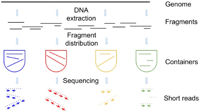
An overview of SLR technologies. A genome (metagenome) is sheared into long fragments that are placed into multiple containers. Fragments in each container are amplified, broken into short subfragments, barcoded and sequenced. Resulting reads are assigned to their original containers using barcodes

As the result, each long fragment is represented as a read cloud: a set of barcoded paired-end reads that originated from a given fragment (Kuleshov et al., 2016).

TSLR and SSLR. The TruSeq SLR (TSLR) technology generates 384 containers with 150–300 fragments with length $\approx 10$kb and sequences them with high coverage (Bankevich and Pevzner, 2016; Voskoboynik et al., 2013). These parameters enable barcode assembly of all reads with the same barcode that aims to reconstruct all fragments marked by this barcode.

Although TSLRs revealed rare species in metagenomes (Bankevich and Pevzner, 2016, 2018; Sharon et al., 2015), their applications are limited by a rather high cost.

The Sparse SLR (SSLR) technologies (such as developed by 10x Genomics and UST) represent a lower cost alternative to the TSLR technology (Marks et al., 2018; Zheng et al., 2016) that results in a low coverage of fragments by short reads and does not enable barcode assembly. Instead, it generates longer fragments (typically 10–70 kb) distributed over many containers (up to 4 million).

In difference from truSPAdes (Bankevich and Pevzner, 2016) aimed at high-cost TSLRs, cloudSPAdes was developed for the lower-cost SSLRs.

The mean fragment length defines a typical repeat length an SSLR technology can resolve. However, the low coverage of fragments by short reads may result in difficulties in repeat resolution, even in the case of long fragments. Thus, each SSLR assembly algorithm should be adapted to the parameters of a specific SSLR technology and even to the parameters of a specific dataset (even generated by the same technology!) since various datasets often have different characteristics.

Although the 10X Genomics Chromium Controller is now the most popular instrument for generating SSLRs, various groups are now developing new barcoding protocols with the goal to reduce the cost of SSLRs and even substitute a rather expensive Chromium Controller by a simpler kit-based barcoding protocol, thus reducing the cost by an order of magnitude. For example, UST recently introduced Transposase Enzyme Linked Long-read Sequencing (TELL-seq^TM) that enables faster and more cost-effective way to generate SSLRs in a single-tube reaction without a need for an expensive protocol-specific instrument. TELL-Seq promises to advance short-read sequencing by replacing mate-pairs in generating low-cost high-quality short-read assemblies.

TELL-seq takes advantage of a unique property of Mu transposition reaction, which creates a very stable intermediate product (i.e. strand transfer complex) when Mu transposomes attack a DNA target (Savilahti et al., 1995), and barcodes the DNA target before it breaks. TELL-Seq produces SSLR sequencing libraries for a variety of genome sizes ranging from bacterium to human with 1 to 10 ng genomic DNA input in approximately 3 h. In difference from the Chromium Controller, it does not require emulsion compartments and results in a scalable and automation-friendly workflow.

Since various barcoding protocols often have different parameters, there is a need to test how these parameters affect the quality of genome assembly. However, our benchmarking revealed that existing SSLR assemblers are optimized for a narrow range of parameters and their performance may greatly deteriorate when these parameters change. With respect to various applications, we demonstrate that the state-of-the-art metagenomics SSLR assemblers, that work well on some dataset, may perform poorly on other datasets with different coverage of fragments by short reads, different distributions of species abundances, etc. For example, even for the same SSLR technology, there exist a need to adjust parameters due to varying sample characteristics, e.g. DNA can be more fragmented in one sample versus another, resulting in shorter fragments. This raises a problem of developing a universal SSLR assembler that learns parameters from the data and works well across a wide range of parameters.

SLR assemblers. The existing SLR assemblers can be classified into three categories:

• The barcode assembly approach reconstructs SLRs by assembling short reads from a single barcode as in the TSLR technology (Bankevich and Pevzner, 2016) or several barcodes as in the SSLR technology (Bishara et al., 2018), and further reconstructs the genome from the resulting SLRs.

• The scaffolding approach aligns the barcoded reads to contigs and uses them for scaffolding (Adey et al., 2014; Kuleshov et al., 2016; Yeo et al., 2018).

• The de Bruijn graph approach constructs the assembly graph of all barcoded reads and uses it for the follow-up SLR assembly (Weisenfeld et al., 2017).

With exception of Supernova (Weisenfeld et al., 2017), the existing SSLR assemblers [Architect (Kuleshov et al., 2016), ARCS (Yeo et al., 2018) and Athena (Bishara et al., 2018)] use SPAdes assembler (Bankevich et al., 2012) for an initial assembly (without using barcoding information) and further improve it by utilizing the barcoding information. However, they only use SPAdes contigs and do not take advantage of the SPAdes assembly graph that provides important information for analyzing barcodes. cloudSPAdes addresses this limitation by analyzing the assembly graph and represents the first application of assembly graphs for metagenomic SSLR assembly [assembly graphs were previously used only for genomic SSLR assembly (Weisenfeld et al., 2017)].

The Shortest Cloud Superstring Problem. A string is called a superstring of a collection of strings if it contains each string from this collection as a substring. The genome assembly problem is related to the Shortest Superstring Problem, finding a shortest superstring for a collection of strings. In difference from the classical genome assembly problem, the algorithmic problems motivated by the SSLR assembly have not been explored yet. Below we describe an analog of the Shortest Superstring Problem (for a set of clouds rather than strings) motivated by the SLR assembly.

The composition of a string S [denoted as composition(S)] is defined as the set of all characters in S. A set of characters c is a cloud of a string S if there exists a substring s of S with composition equal to c. We say that a string S conforms with a collection of sets C (referred to as a cloud-set) if each set in C is a cloud of S. Given a cloud-set C, the Shortest Cloud Superstring (SCS) Problem is to find a shortest string that conforms with C. Note the difference between the Shortest Superstring (the set of strings is known) and the SCS Problems (the set of strings is unknown but their compositions are known), reflecting the difference between the classical genome assembly and the SLR assembly.

Below we explain how the SCS Problem relates to the SLR assembly, describe an algorithm for solving this problem, generalize this problem for assembly graphs and use it to develop the cloudSPAdes tool for both genomics and metagenomic SSLR assembly.

2 Materials and methods

De Bruijn graph. In the genomic mode, cloudSPAdes uses a genomic assembler SPAdes (Bankevich et al., 2012) to construct the assembly graph from reads. Given a set of reads Reads and a k-mer size (or a range of k-mer sizes in the iterative mode), SPAdes constructs the de Bruijn graph of reads and transforms it into the assembly graph$\mathit{DB}=\mathit{DB}(\mathit{Reads},k)$ after performing various graph simplification procedures (Fig. 2). In the metagenomic mode, cloudSPAdes uses a metagenomic assembler metaSPAdes (Nurk et al., 2017) to construct the assembly graph from reads with non-uniform coverage.

Fig. 2.

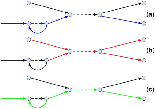
Outline of the cloudSPAdes algorithm. (First layer) Linear representation of a circular genome $a{s}_1{s}_{2}b{s}_{4}c{s}_3{s}_{2}d{s}_1{s}_{2}e{s}_4$ with five long edges $a,b,c,d$ and e. Numbers under the edges denote the lengths of the segments. (Second layer left) Assembly graph DB of the genome. (Second layer right) Contracted assembly graph CDB. The contraction of an edge (v, w) is the gluing of the endpoints of this edge into a single vertex u, followed by the removal of the loop-edge resulting from this gluing (all edges incident to v or w in the assembly graph are incident to u in the contracted assembly graph). (Third layer left) The containment metric for the contracted de Bruijn graph CDB. (Third layer middle) The transition-set T in the contracted assembly graph with the containment index exceeding 0.7 and the T-compatible cloud-set C. The transition-set T includes all correct genomic transitions (ab, bc, cd, de, ea) and three false transitions (ba, cb, ae). (Third layer right) The T-compatible clouded Eulerian cycle for the contracted assembly graph CDB, the transition-set T and the cloud-set C. (Fourth layer) The short-edge subgraph of the assembly graph DB between two consecutive long edges a and b in the genomic cycle. There are two possible ways to fill the gap between a and b, the correct one (shown on top and reconstructed by cloudSPAdes) and the incorrect one (shown at the bottom)

Each edge in the assembly graph is labeled by a nucleotide string and the length of an edge is defined as the number of nucleotides in this string.

For simplicity, below we assume that all chromosomes are circular. Each chromosome traverses a cycle in the assembly graph that we refer to as a genomic cycle (a genomic cycle may be broken into multiple paths if there exist drops in coverage that fragment the assembly graph). The multiplicity of an edge in the assembly graph is defined as the total number of times it is traversed by all genomic cycles in the assembly graph. An edge is classified as unique if its multiplicity is 1 and as repeat, otherwise. Although this classification is not known in the de novo setting, SPAdes infers the tentative sets of unique and repeat edges.

Clouds in the assembly graph. We refer to a subpath of the genomic cycle traversed by a fragment F in the assembly graph DB as path(DB, F) and to the set of edges in this subpath as the cloud in the assembly graph of the fragment F, referred to as cloud(DB, F). We say that a barcode marks an edge of the assembly graph if one of the reads aligned to this edge has this barcode. We refer to a barcode marking the fragment F as barcode(F).

In the ideal case, when barcode(F) marks all edges in path(DB, F) (and does not mark other edges), the SSLR technology provides information about cloud(DB, F) [all edges marked by barcode(F)] but does not reveal path(DB, F). In practice, if edges of cloud(DB, F) form a connected subgraph in the assembly graph, one might attempt to reconstruct path(DB, F) from cloud(DB, F) as a path traversing all edges in this subgraph. If we succeed in reconstructing path(DB, F), we can transform it into a string over the edge alphabet (the set of all edges in the assembly graph). If all fragments were transformed into such strings, the SSLR assembly problem would be reduced to genome assembly from a set of such strings.

In reality, path(DB, F) may be self-overlapping (in the case when it contains repeat edges), making it difficult to figure out how it traverses edges in cloud(DB, F). Below we show how to use clouds for reconstructing the genomic cycle even in the case when paths traversed by some fragments are unknown.

Since each cloud in the assembly graph is a composition of a subpath of a genomic cycle, the SSLR assembly corresponds to solving the SCS Problem for the set of all clouds in the assembly graph. However, although the SCS Problem is a useful abstraction, it does not adequately model the cloud assembly (similarly to the Shortest Superstring Problem that does not adequately model the read assembly).

Below we introduce a more adequate model for the SSLR assembly [Clouded Eulerian Path (CEP) problem] and describe a practical SSLR assembly algorithm.

The challenge of reconstructing clouds in the assembly graph. Given the set of all edges marked by barcode [referred to as edges(DB, barcode)], we consider the problem of reconstructing cloud(DB, F) for all fragments F marked by barcode.

One way to address this problem is to select each connected subgraph formed by edges(DB, barcode) as an approximation of cloud(DB, F) for some fragment F. However, short edges in cloud(DB, F) are often not marked by barcode(F) (since the coverage of fragments by reads is low), making it difficult to reconstruct cloud(DB, F). In this case, cloud(DB, F) does not form a connected subgraph in the assembly graph and is broken into multiple connected subgraphs (Fig. 3a).

Fig. 3.

Reconstructing clouds in the assembly graph. A fragment of assembly graph with edges marked by blue, red and green barcodes. Long edges are shown as solid and short edges are shown dashed. (a) A cloud formed by the blue barcode is broken into two subgraphs. (b) Two fragments that share the red barcode also share a short edge, resulting in a multicloud subgraph. (c) A short edge in the fragment-path that is not marked by the green barcode results in a connected component (marked by the green barcode) that cannot be traversed by a single path

Additionally, each barcode usually marks multiple fragments that may correspond to paths sharing some edges. Thus, a connected subgraph formed by edges(DB, barcode) may correspond to several fragments rather than to a single fragment (Fig. 3b). We refer to such subgraphs of the assembly graph as multicloud subgraphs as opposed to unicloud subgraphs that represent a single cloud in the assembly graph.

Since multicloud subgraphs are difficult to analyze, one can consider only subgraphs that form a path [such a path likely corresponds to path(DB, F)] that traverses each edge in a subgraph at least once. However, limiting analysis to paths may filter out some unicloud subgraphs, since some edges unmarked by barcode(F) will be missing from path(DB, F) (Fig. 3c).

Focusing on long edges of the assembly graph. To address the complications illustrated in Figure 2, instead of considering all edges of the assembly graph, we focus on long edges (longer than a length threshold LT) and ignore short edges. We refer to a cloud with at least two long edges as a multi-edge cloud and define the complexity of a cloud-set as the mean number of long edges in a multi-edge cloud. On the one hand, setting up a small length threshold results in difficult-to-analyze cloud-sets with high complexity. On the other hand, setting up a large length threshold results in easy-to-analyze cloud-sets with small complexity but makes it difficult to fill the gaps between consecutive long edges (formed by short edges) in the genomic path.

Our benchmarking revealed that selecting the length threshold in such a way that the resulting clouds are relatively small (the complexity of the resulting cloud-set is $\approx$3) represents a good trade-off. Figure 4 illustrates how the number of long edges and the complexity of a cloud-set [denoted complexity(LT)] reduce with the increase in the length threshold LT. We define the parameter LT as the maximum value L of the length threshold with complexity(L) above 3.

Fig. 4.

Number of long edges in the assembly graph (left), complexity (middle) and the mean weight of a vertex in the contracted assembly graph (right) depending on the edge length threshold (for the YEAST dataset described in Section 3). Long edges are defined as edges longer than 11 kb (the mean number of long edges in a multi-edge cloud is 3 for the edge length threshold 11 kb)

cloudSPAdes first attempts to infer the order of long edges and afterwards attempts to fill the gaps between long edges by progressively shorter and shorter edges.

For simplicity, below we define this iterative process by defining only two tiers of edges lengths: long (longer than LT) and short (all remaining edges). In the Supplementary Material, we will illustrate this iterative process in more details by defining three tiers of edge lengths: ultralong (longer than LT⁺), long (longer than a threshold LT but shorter or equal than LT⁺) and short (all remaining edges).

Contracted assembly graph. Short edges in Path(F) are less likely to be marked by barcode(F) than long edges. Thus, instead of reconstructing the order of all edges in path(DB, F), we focus on a simpler problem of reconstructing the order of long edges in path(DB, F) for every fragment F.

To focus on long edges in the assembly graph DB, we contract all short edges in this graph (Figure 2). Note that the resulting assembly graph may contain non-branching vertices (vertices with a single incoming and a single outgoing edge). The contracted assembly graph DB_LT is obtained from this graph by transforming each non-branching path into a single edge. For the YEAST dataset ($\mathit{LT}\approx 11$ kb), the contracted assembly graph DB_LT has 154 vertices and 525 edges (13 of them are loops). We define the weight of a vertex in the contracted assembly graph as the total length of all edges that were contracted into this vertex (Fig. 4).

Below we describe variations of the SCS Problem aimed at analyzing the contracted assembly graph [Cloud Permutation (CP) Problem and CEP Problem]. The latter employs the concept of transitions between the edges of the contracted assembly graph that we use for reconstructing the set of long edges for every cloud in the assembly graph. A transition-set in a graph G is an arbitrary set of pairs of incident edges (v, w) and (w, u) in this graph [a loop (v, v) may form a transition with any edge that has v as one of its endpoints]. We distinguish between correct transitions (pairs of consecutive edges in a genomic path) and false transitions (all other pairs of edges).

The CP Problem and the CEP Problem. Our goal is to solve the SCS Problem for clouds encoded in the alphabet of long edges in the contracted assembly graph. Since long edges are mostly unique, this task corresponds to a simpler CP Problem: find a permutation (a string without repeated symbols) that conforms with a cloud-set C. We omitted the word ‘shortest’ in this formulation, since all permutations have the same length [each of them contains all characters from C that we denote as char(C)].

Twenty years ago, various DNA physical mapping studies (Pevzner, 2000; Rajaraman et al., 2017) analyzed algorithmic problems similar to the CP Problem (Alizadeh et al., 1995; Batzoglou and Istrail, 1999; Mayraz and Shamir, 1999). However, we are not aware of a software tool that resulted from these studies and would be applicable to SSLRs. Below we describe the CEP Problem that is relevant to analyzing clouds on edges of an assembly graph.

We refer to a cloud-set where each cloud is a subset of edges in a graph G as a cloud-set in G. Given a transition-set T in a graph G, we say that a path P in G is T-compatible, if every pair of consecutive edges in this path forms a transition in T. Given a transition-set T in a graph G, and a cloud-set C in G, a Clouded Eulerian Path is a T-compatible Eulerian path in G that forms a permutation of its edges conforming with the cloud-set C. The CEP Problem is to find a CEP for G, T and C. Note that solving the Clouded Permutation Problem on C is equivalent to solving the CEP problem in the case when a graph G contains a single vertex, all its edges represent loops, and every pair of edges in G forms a transition. In the case of an empty cloud-set C, solving the CEP problem corresponds to finding a T-compatible Eulerian path in G (Fleischner, 1990).

Clouds in the contracted assembly graph. Each cloud cloud(DB, F) in the assembly graph corresponds to a cloud cloud(CDB, F) in the contracted assembly graph. Let clouds(CDB, barcode) be the set of clouds in the contracted assembly graph of all fragments marked by barcode. Since the contracted assembly graph does not have short edges [that are often not marked by barcode(F)], clouds in this graph are more likely to represent connected subgraphs than clouds in the assembly graph. Thus, reconstructing clouds(CDB, barcode) from only long edges marked by barcode is easier than reconstructing clouds(DB, barcode) from all edges in the assembly graph marked by barcode.

Each barcode marks a set of edges edges(CDB, barcode) in the contracted assembly graph. We consider the induced subgraph formed by these edges and analyze its connected components. Given a transition-set T, we classify a connected component as simple if it contains a T-compatible Eulerian path (non-simple components likely result from barcode collisions) and report simple components as putative clouds. We refer to the set of putative clouds constructed using the contracted assembly graph CDB, a transition-set T and barcoded reads Reads as $\mathit{Clouds}(\mathit{CDB},T,\mathit{Reads})$ (each cloud in this set represents a set of edges in the contracted assembly graph).

Let Genome be a genome string and Cycle(Genome, DB) be a genomic cycle traversed by Genome in the assembly graph DB. This cycle got contracted into a genomic cycle Cycle(Genome, CDB) in the contracted assembly graph CDB that we aim to reconstruct. Given a contracted assembly graph CDB, we attempt to solve the cloud superstring problem for the cloud-set $\mathit{Clouds}(\mathit{CDB},T,\mathit{Reads})$ to reconstruct Cycle(Genome, CDB).

Brief outline of the cloudSPAdes algorithm. Below we use a simple simulated dataset to illustrate the main steps of the algorithm and delegate the details to the Supplementary Material. Figure 2 describes a simulated genome and a simulated SSLR dataset with 50 000 fragments (with mean fragment length 20 kb and mean coverage 0.1×) distributed among 2000 containers.

cloudSPAdes first derives the parameter LT by analyzing the dataset and uses it to transform the assembly graph DB into the contracted assembly graph $\mathit{CDB}=D{B}_{\mathit{LT}}$. It further defines the initial transition-set that includes five correct (ab, bc, cd, de, ea) and seven false (ad, ae, ba, cb, ce, db, ec) transitions. cloudSPAdes attempts to remove false transitions by evaluating various metrics described in the Supplementary Material. Figure 2 illustrates only one of these metrics that we describe below.

We refer to the set of barcodes marking an edge e in a graph as barcode-set of an edge and denote this set as b(e). Given edges e₁ and e₂, we refer to the set of barcodes marking both e₁ and e₂ as $b(e_1,e_2)$. We score the similarity between barcode-sets of two edges using the containment index CI (Koslicki and Zabeti, 2017)

$$\text{CI}(e_1,e_2)=\frac{|b(e_1,e_2)|}{\text{min}(|b(e_1)|,|b(e_2)|)}.$$

We say that long edges e₁ and e₂ have similar barcode-sets if $\text{CI}(e_1,e_2)$ exceeds a threshold CI_long (the approach for setting this threshold is described in the Supplementary Material).

Figure 2 shows the containment metric for the simulated dataset (entries exceeding the threshold CI_long are shown in dark blue). After applying this threshold, we are left with a transition-set T consisting of all correct transitions (ab, bc, cd, de, ea) and three false transitions (ba, cb, ae). After deriving the transition-set T, cloudSPAdes constructs a cloud-set $C=\mathit{Clouds}(\mathit{CDB},T,\mathit{Reads})$ in the contracted assembly graph consisting of only five clouds {ab}, {bc}, {abe}, {bcd}, {cde}. Afterwards, cloudSPAdes attempts to find out how the genomic cycle traverses the contracted assembly graph by solving the CEP problem (there exists only one T-compatible Eulerian cycle for this cloud-set).

After finding a genomic cycle in the contracted assembly graph CDB, cloudSPAdes turns the attention to the assembly graph DB, fills the gap between each pair of consecutive long edges in this cycle and constructs a genomic cycle in the assembly graph. In the simulated example, it is not clear whether this cycle is traversed as $a{s}_1{s}_{2}b{s}_{4}c{s}_3{s}_{2}d{s}_1{s}_{2}e{s}_4$ or as $a{s}_3{s}_{2}b{s}_{4}c{s}_1{s}_{2}d{s}_1{s}_{2}e{s}_4$. cloudSPAdes selects one of these possibilities by iteratively reducing the parameter LT to fill the gaps between long edges in the assembly graph using additional metrics described in the Supplementary Material.

Combinatorics of crossing clouds. cloudSPAdes is motivated by a combinatorial analysis of cloud-sets that we describe in the Supplementary Material. For simplicity, the theoretical results below and in the Supplementary Material refer to the case of reconstructing a single linear genome. However, in the case of a metagenome, cloudSPAdes uses these results to assemble multiple circular genomes in a metagenome. For a self-contained description of all results, below we define a condition on a cloud-set that guarantees that the CP Problem has a unique solution.

We say that sets c₁ and c₂cross ($c_1⌢c_2$) iff $c_1\cancel{\subseteq }{c}_2,\hspace{0.17em}{c}_2\cancel{\subseteq }{c}_1$, and $c_1\cap c_2\ne \varnothing$. A cloud-set C crosses a subset of char(C) if it contains a cloud crossing this subset. A set of clouds C is complete if it crosses each non-trivial subset of char(C).

Theorem. Let G be a permutation that conforms with a cloud-set C. Then G is unique iff C is complete.

Organization of Supplementary Material. Section 1 introduces various procedures aimed at eliminating false transitions. Sections 2–7 describe the transition elimination procedures in more details. Section 8 describes how to partition the contracted assembly graph into smaller subgraphs and to solve a separate CP Problem in each of them. Section 9 describes how cloudSPAdes utilizes read-pairs in the SSLR libraries.

Long edges in path(DB, F) form a path path(CDB, F) in the contracted assembly graph that we aim to reconstruct and to further use the reconstructed paths for figuring out how the genomic cycle traverses the contracted assembly graph. Since path(CDB, F) does not provide information about short edges within genomic cycle, Supplementary Section 10 describes how to fill in the gaps between long edges in this path (formed by paths consisting of short edges), thus reconstructing the entire genomic cycles.

The proof of the Theorem is given in Supplementary Section 11. Supplementary Sections 12 and 13 describe how cloudSPAdes combines information provided by a cloud-set and a transition-set in the contracted assembly graph. Supplementary Section 14 outlines the steps of the cloudSPAdes algorithms in more details.

3 Results

SLR assemblers. We benchmarked cloudSPAdes and the state-of-the-art SSLR assemblers Architect (Kuleshov et al., 2016), ARCS (Yeo et al., 2018), Athena (Bishara et al., 2018) and Supernova (Weisenfeld et al., 2017) using QUAST (Gurevich et al., 2013) and metaQUAST (Mikheenko et al., 2016). Architect, ARCS, Athena and Supernova are aimed at various settings and/or various variants of the SLR technologies: Architect is best suited for TSLR assemblies, ARCS and Supernova were developed for human SSLR assemblies and Athena was developed for metagenomics SSLR assemblies.

Datasets. We benchmarked all SLR assemblers on three genomic SSLR dataset generated by TELL-seq technology and three metagenomic SSLR datasets generated by 10X Genomics technology (see Supplementary Section 15 for detailed information about these datasets and the reference genomes). Although the metagenomics datasets were generated using the same, they have widely different characteristics with respect to fragment coverage by short reads and abundances of various species, thus allowing us to analyze how stable each assembly tool is with respect to these variations. The genomic datasets were analyzed with the goal to evaluate whether the state-of-the-art SSLR tools can be applied to emerging technologies with parameters that differ from the parameters of the 10X Genomics technology.

YEAST, STAPH and ECOLI datasets contain reads from the genomic DNA of Saccharomyces cerevisiae, Staphylococcus aureus and Escherichia coli DH10B strain, respectively.

MOCK5 dataset is a synthetic community dataset containing reads from the genomic DNA mixture of five bacterial species, four of them have genomes that are similar to known genomes (Danko et al., 2019).

MOCK20 dataset is a synthetic community dataset containing reads from the genomic DNA mixture of 20 bacterial strains, 19 of them have genomes that are similar to known genomes (Bishara et al., 2018).

GUT dataset is a large metagenomic dataset from the gut of a male adult (Bishara et al., 2018).

The lengths of fragments generated by the SSLR technology are defined by the lengths of DNA fragments extracted from the sample.

Since extracting high molecular weight DNA from a metagenomic sample is challenging (Bag et al., 2016; Kuhn et al., 2017), the average SSLR fragment length often drops from 30–70 kb in an isolate to 5–10 kb in a metagenome. Supplementary Section 16 presents statistics for various SSLR metagenomic datasets.

Benchmarking SLR assemblers. Table 1 summarizes the assembly statistics for metagenomic datasets. Table 2 summarizes the assembly statistics for prokaryotic datasets. Figure 5 presents the NAx plots for the YEAST, STAPH, ECOLI, MOCK5 and MOCK20 datasets and the NGx plot for the GUT dataset. Figure 6 provides information about the NGA50 statistics and the number of misassemblies for each reference genome for the MOCK5, MOCK20 and GUT datasets.

Table 1.

Assembly statistics for the MOCK5, MOCK20 and GUT datasets

Assembler	metaSPAdes	Athena	cloudSPAdes	Architect	ARCS	Supernova
MOCK5
# contigs	353	117	97	295	319	1895
Total length (kb)	21 253	21 820	21 260	21 259	21 256	21 614
NA50 (kb)	51	154	225	61	52	2
N50 (kb)	116	351	1294	185	168	120
NA10 (kb)	194	688	1265	284	268	101
N10 (kb)	562	1020	2836	1129	1372	2369
Longest alignment (kb)	268	1150	1416	563	563	491
# N’s per 100 kb	22	0	761	25	23	15 762
Mean NGA50 per reference (kb)	93	544	528	125	105	19
Mean # misassemblies per reference	3.75	21.5	10	5.25	6.25	59.5
Running time	37 h	37 h + 36 h	37 h + 51 min	37 h + 4 h	37 h + 3.5 h	25 min
MOCK20
# contigs	1089	243	793	1032	1015	13 193
Total length (kb)	51 053	50 917	54 838	51 067	51 060	67 321
NA50 (kb)	50	203	124	50	54	18
N50 (kb)	155	885	845	157	189	36
NA10 (kb)	364	1141	1368	366	1021	95
N10 (kb)	581	3011	1968	587	6300	166
Longest alignment (kb)	907	2389	1844	907	1435	1532
# N’s per 100 kb	14	0.4	403	16	14	245
Mean NGA50 per reference (kb)	153	781	787	153	467	343
Mean # misassemblies per reference	1.4	3.4	3.0	1.6	1.6	12.2
Running time	68 h	68 h + 9 days	68 h + 3 h	68 h + 6.5 h	68 h + 5 h	26 days
GUT
# contigs	39 317	14 015	33 130	39 283	39 270	25 333
Total length (kb)	342 982	318 979	376 934	346 276	342 987	374 906
NG50	5708	15 544	12 729	5903	6441	21 195
NG10	95 914	375 559	322 007	96 072	95 939	263 602
Longest contig (kb)	725	1968	1934	725	725	1787
# N’s per 100 kb	22	0	714	22	23	22 613
Mean NGA50 per reference	40 301	93 563	85 859	40 301	40 301	17 586
Mean # misassemblies per reference	11.08	52.46	35.31	13.69	11.15	24.53
Running time	6 days	6 days + 24 days	6 days + 12.5 h	6 days + 13 h	6 days + 9 h	28 h

Note: The running time for all tools but Supernova includes the SPAdes or metaSPAdes running time ($\approx 6$ days for the GUT dataset). The best value for each row is indicated in bold. metaSPAdes was run with the default k-mer size equal to 55. All benchmarking was done on Intel Xeon E7-4880 processor using 15 CPUs. metaQUAST defines the NA50 statistics as similar to NGA50, but calculates it with respect to the total assembly length instead of the reference genome size. To compare various assemblers, we used both contigs and scaffolds exceeding 2 kb in length. metaQUAST was launched with the -m 2000 and -x 2500 options for all datasets, and with –fragmented option for the GUT dataset. The reference length for the GUT dataset was set to length of the metaSPAdes assembly (520 Mb). Since the reference assemblies may have significant differences compared to the genomes in the GUT metagenome, estimates of the number of assembly errors for the GUT dataset should be taken with caution since many of the errors may represent differences with the references rather than errors. All tools except Architect were run with default parameters. Architect was run with parameters t = 2, $\mathit{rc}\_\mathit{abs}\_\mathit{thr}=3,\hspace{0.17em}\mathit{rc}\_\mathit{rel}\_\mathit{edge}\_\mathit{thr}=0.02,\hspace{0.17em}\mathit{rc}\_\mathit{rel}\_\mathit{prun}\_\mathit{thr}=0.01$ to optimize its performance on SSLR datasets.

Table 2.

Assembly statistics for the YEAST, STAPH and ECOLI datasets

Assembler	SPAdes	Athena	cloudSPAdes	Architect	ARCS	Supernova
YEAST
# contigs	305	116	101	320	259	898
Total length (kb)	11 583	11 752	11 734	11 603	11 589	10 983
NGA50 (kb)	103	179	539	228	185	22
NG50 (kb)	103	187	691	410	198	23
NGA10 (kb)	227	470	888	622	532	63
NG10 (kb)	243	470	1, 715	772	533	70
Longest alignment (kb)	314	545	848	314	584	92
# N’s per 100 kb	18	1	761	24	57	548
# misassemblies	1	15	7	21	1	16
Running time	74 min	74 min + 11 h	74 min + 13 min	74 min + 30 min	74 min + 42 min	25 min
STAPH
# contigs	89	21	56	75	79	12
Total length (kb)	2870	2886	2905	2874	2872	2957
NGA50 (kb)	174	728	1645	821	252	2794
NG50 (kb)	174	728	1655	821	252	2797
NGA10 (kb)	303	1170	1645	859	356	2794
NG10 (kb)	313	1231	1654	1022	356	2797
Longest alignment (kb)	313	1170	1645	859	356	2793
# N’s per 100 kb	25	0	603	33	60	27
# misassemblies	2	2	3	5	2	0
Running time	119 min	119 min + 115 min	119 min + 1 min	119 min + 11 min	119 min + 9 min	190 min
ECOLI
# contigs	110	16	9	75	75	63
Total length (kb)	4515	4634	4596	4516	4518	4471
NGA50 (kb)	82	396	2543	201	287	123
NG50 (kb)	83	439	2813	209	287	127
NGA10 (kb)	260	1, 075	2543	542	505	260
NG10 (kb)	260	1, 075	2813	542	506	260
Longest alignment (kb)	326	1074	2543	542	505	414
# N’s per 100 kb	20	0	647	28	97	73
# misassemblies	1	5	3	5	3	5
Running time	18 min	18 min + 43 min	18 min + 11 s	18 min + 1 min	18 min + 53 s	11 min

Note: The running time for all tools but Supernova includes the SPAdes running time. The best value for each row is indicated in bold. All benchmarking was done on Intel Xeon E7-4880 processor using 15 CPUs. Number of misassemblies includes only global misassemblies as identified by QUAST (with breakpoint distance exceeding 2 kb). QUAST was launched with the –scaffold-gap-max-size 20000 and -x 2000 options for all datasets.

Fig. 5.

The NGAx plots for the YEAST (top left), STAPH (top middle) and ECOLI(top right) datasets. NAx plots for the MOCK5 (top right), NAx plots for the MOCK20 (bottom left) and NGx plot for the GUT (bottom right) datasets. The metaSPAdes curve is not shown since it is nearly identical to the ARCS curve for the GUT dataset. The metaSPAdes curve is replaced with the SPAdes curve for the YEAST, STAPH and ECOLI plots

Fig. 6.

metaQUAST statistics for MOCK5, MOCK20 and GUT datasets. NGA50 statistics per reference for the MOCK5(top left), MOCK20 (top middle) and GUT(top right) datasets. Number of misassemblies per reference for the MOCK5 (bottom left), MOCK20 (bottom middle) and GUT (bottom right) datasets. Genomes are represented by their RefSeq IDs

The benchmarking results for the YEAST datasets reveal that the existing SSLR assemblers are unstable with respect to parameters: their performance deteriorates when they are faced with datasets whose parameters differ from the parameters these assemblers optimized for. The unstable behavior of various SSLR tools makes it difficult to develop new barcoding technologies since the ongoing experimental developments of new protocols have to be constantly complemented by computational tests (otherwise it is unclear how a new technology affects the downstream assembly).

cloudSPAdes turned out to be a fast assembler that performs well across the range of technologies and applications. As discussed in (Nurk et al., 2017), the NA50 metric alone is limited with respect to estimating the contiguity of metagenomics assemblers since biologists are typically interested in the contiguity of the 10–100 most abundant genomes that often form less than 50% of the total metagenome length. We thus reflected the both NA50 and NA10 statistics in Table 1 (see Fig. 5 for detailed information about the contiguity of various assemblers).

On the MOCK5 dataset, cloudSPAdes generated the longest contigs with respect to the NA50 (225 kb for cloudSPAdes versus 154 kb for Athena) and NA10 (1265 kb versus 688 kb). The superior performance of cloudSPAdes on the MOCK5 dataset may be explained by its adaptability to the specific properties of the SSLR datasets, e.g. the MOCK5 dataset has an unusually low fragment coverage.

On the MOCK20 datasets, cloudSPAdes and Athena showed similar results: Athena resulted in higher NA50 (124 kb for cloudSPAdes versus 203 kb for Athena) but lower NA10 (1368 kb for cloudSPAdes versus 1141 kb for Athena).

On the GUT dataset, cloudSPAdes, Athena and Supernova generated the most contiguous assemblies. However, Supernova’s assembly has limited applicability since it generated contigs with an extremely large fraction of unknown nucleotides (22.6% of all nucleotides are marked as Ns). cloudSPAdes and Athena resulted in assemblies with similar contiguity (NG50 and NG10 are approximately 20% higher for Athena than for cloudSPAdes). However, NG50 and NG10 parameters do not account for assembly errors that typically inflate the contig lengths. Since only a few reference genomes for the GUT dataset are known, we are unable to derive the NA50 and NA10 statistics for this dataset. However, judging from the fact that Athena made $\approx$50% more assembly errors on the reference GUT genomes, we project that cloudSPAdes assemblies may have very similar or even higher NA50 and NA10 statistics than Athena assembly. Interestingly, Athena resulted in a 20% smaller total assembly length than cloudSPAdes. Athena took 24 days to assemble the GUT dataset, while cloudSPAdes took only 12.5 h (not counting the metaSPAdes running time).

4 Discussion

Although long error-prone reads have revolutionized sequencing of large genomes, the relatively high cost limits their applications to sequencing of small genomes. This is unfortunate since the number of bacterial sequencing projects based on short reads [most of them assembled with SPAdes (Bankevich et al., 2012)] greatly exceeds the number of eukaryotic sequencing projects based on long reads [most of them assembled with Canu (Koren et al., 2017)]. However, since long-read assemblies are much more contiguous than short-read assemblies, there is an effort to make assemblies of small genomes both contiguous and cost efficient at the same time. Although SSLRs represent a potential solution for a low-cost genome sequencing, the 10X Genomics Chromium Controller remains rather expensive for sequencing small genomes. That is why UST and other companies are trying to reduce the cost of SSLRs, to eliminate the need for an expensive Chromium Controller, to simplify sample preparation, and to enable new SSLR applications. These efforts promise to revolutionize sequencing of small genomes by making it as cost-effective as short-read sequencing and as contiguous as long read sequencing. However, to support such developments, there is a need to develop a ‘universal’ SSLR assembler that works well across various barcoding technologies and various applications.

We have demonstrated that the existing SSLR assemblers are rather stringent with respect to changing parameters of the emerging barcoding technologies and even the parameters of specific metagenomics datasets generated using the same 10X Genomics technology. cloudSPAdes is an attempt to develop a universal open-source SSLR assembler that works well across various technologies and datasets. Although it significantly improves on the contiguity of SPAdes and metaSPAdes assemblies, further efforts are needed to close the gap between the contiguity (and the number of assembly errors) of the low-cost SSLR assemblies and high-cost assemblies based on long error-prone reads.

References

- Adey A. et al. (2014) In vitro, long-range sequence information for De Novo genome assembly via transposase contiguity. Genome Res., 24, 2041–2049. [DOI] [PMC free article] [PubMed] [Google Scholar]
- Alizadeh F. et al. (1995) Physical mapping of chromosomes: a combinatorial problem in molecular biology. Algorithmica, 13, 52–76. [Google Scholar]
- Bag S. et al. (2016) An improved method for high quality metagenomics DNA extraction from human and environmental samples. Sci. Rep., 6, 26775.. [DOI] [PMC free article] [PubMed] [Google Scholar]
- Bankevich A., Pevzner P.A. (2016) TruSPAdes: barcode assembly of TruSeq synthetic long reads. Nat. Methods, 13, 248–250. [DOI] [PubMed] [Google Scholar]
- Bankevich A., Pevzner P.A. (2018) Joint analysis of long and short reads enables accurate estimates of microbiome complexity. Cell Syst., 7, 192–200. [DOI] [PubMed] [Google Scholar]
- Bankevich A. et al. (2012) SPAdes: a new genome assembly algorithm and its applications to single-cell sequencing. J. Comput. Biol., 19, 455–477. [DOI] [PMC free article] [PubMed] [Google Scholar]
- Batzoglou S., Istrail S. (1999) Physical mapping with repeated probes: the hypergraph superstring problem In: Crochemore, M. and Paterson, M. (eds) Combinatorial Pattern Matching. CPM 1999. Lecture Notes in Computer Science, Vol. 1645. Springer, Berlin, Heidelberg, pp. 66–77. [Google Scholar]
- Bishara A. et al. (2018) High-quality genome sequences of uncultured microbes by assembly of read clouds. Nat. Biotechnol., 36, 1067–1075. [DOI] [PMC free article] [PubMed] [Google Scholar]
- Danko D.C. et al. (2019) Minerva: an alignment- and reference-free approach to deconvolve linked-reads for metagenomics. Genome Res., 29, 116–124. [DOI] [PMC free article] [PubMed] [Google Scholar]
- Fleischner H. (1990) Eulerian Graphs and Related Topics, Vol. 1. Elsevier, Amsterdam. [Google Scholar]
- Gong L. et al. (2018) Culture-independent analysis of liver abscess using nanopore sequencing. PLoS One, 13, e0190853.. [DOI] [PMC free article] [PubMed] [Google Scholar]
- Goordial J. et al. (2017) In situ field sequencing and life detection in remote (79–26’N) Canadian high arctic permafrost ice wedge microbial communities. Front. Microbiol., 8, 2594.. [DOI] [PMC free article] [PubMed] [Google Scholar]
- Gurevich A. et al. (2013) QUAST: quality assessment tool for genome assemblies. Bioinformatics, 29, 1072–1075. [DOI] [PMC free article] [PubMed] [Google Scholar]
- Koren S. et al. (2017) Canu: scalable and accurate long-read assembly via adaptive k-mer weighting and repeat separation. Genome Res., 27, 722–736. [DOI] [PMC free article] [PubMed] [Google Scholar]
- Koslicki D., Zabeti H. (2017) Improving min hash via the containment index with applications to metagenomic analysis. Preprint.
- Kuhn R. et al. (2017) Comparison of ten different DNA extraction procedures with respect to their suitability for environmental samples. J. Microbiol. Methods, 143, 78–86. [DOI] [PubMed] [Google Scholar]
- Kuleshov V. et al. (2016) Genome assembly from synthetic long read clouds. Bioinformatics, 32, i216–i224. [DOI] [PMC free article] [PubMed] [Google Scholar]
- Marks P. et al. (2018) Resolving the full spectrum of human genome variation using linked-reads. Genome Res., 29, 635–645. [DOI] [PMC free article] [PubMed] [Google Scholar]
- Mayraz G., Shamir R. (1999) Construction of physical maps from oligonucleotide fingerprints data. J. Comput. Biol., 6, 237–252. [DOI] [PubMed] [Google Scholar]
- Mikheenko A. et al. (2016) MetaQUAST: evaluation of metagenome assemblies. Bioinformatics, 32, 1088–1090. [DOI] [PubMed] [Google Scholar]
- Nurk S. et al. (2017) metaSPAdes: a new versatile metagenomic assembler. Genome Res., 27, 824–834. [DOI] [PMC free article] [PubMed] [Google Scholar]
- O’Leary N.A. et al. (2016) Reference sequence (RefSeq) database at NCBI: current status, taxonomic expansion, and functional annotation. Nucleic Acids Res., 44, D733–D745. [DOI] [PMC free article] [PubMed] [Google Scholar]
- Ondov B.D. et al. (2016) Mash: fast genome and metagenome distance estimation using MinHash. Genome Biol., 17, 132.. [DOI] [PMC free article] [PubMed] [Google Scholar]
- Pevzner P. (2000) Computational Molecular Biology: An Algorithmic Approach. The MIT Press, Cambridge, MA. [Google Scholar]
- Rajaraman A. et al. (2017) Algorithms and complexity results for genome mapping problems. IEEE/ACM Trans. Comput. Biol. Bioinformatics, 14, 418–430. [DOI] [PubMed] [Google Scholar]
- Savilahti H. et al. (1995) The phage Mu transpososome core: DNA requirements for assembly and function. EMBO J., 14, 4893–4903. [DOI] [PMC free article] [PubMed] [Google Scholar]
- Sharon I. et al. (2015) Accurate, multi-kb reads resolve complex populations and detect rare microorganisms. Genome Res., 25, 534–543. [DOI] [PMC free article] [PubMed] [Google Scholar]
- Voskoboynik A. et al. (2013) The genome sequence of the colonial chordate, Botryllus schlosseri. Elife, 2, e00569.. [DOI] [PMC free article] [PubMed] [Google Scholar]
- Weisenfeld N.I. et al. (2017) Direct determination of diploid genome sequences. Genome Res., 27, 757–767. [DOI] [PMC free article] [PubMed] [Google Scholar]
- Yeo S. et al. (2018) ARCS: scaffolding genome drafts with linked reads. Bioinformatics, 34, 725–731. [DOI] [PMC free article] [PubMed] [Google Scholar]
- Zheng G.X.Y. et al. (2016) Haplotyping germline and cancer genomes with high-throughput linked-read sequencing. Nat. Biotechnol., 34, 303–311. [DOI] [PMC free article] [PubMed] [Google Scholar]
Associated Data
This section collects any data citations, data availability statements, or supplementary materials included in this article.