

Abstract
Motivation
Predictive models are a powerful tool for solving complex problems in computational biology. They are typically designed to predict or classify data coming from the same unknown distribution as the training data. In many real-world settings, however, uncontrolled biological or technical factors can lead to a distribution mismatch between datasets acquired at different times, causing model performance to deteriorate on new data. A common additional obstacle in computational biology is scarce data with many more features than samples. To address these problems, we propose a method for unsupervised domain adaptation that is based on a weighted elastic net. The key idea of our approach is to compare dependencies between inputs in training and test data and to increase the cost of differently behaving features in the elastic net regularization term. In doing so, we encourage the model to assign a higher importance to features that are robust and behave similarly across domains.
Results
We evaluate our method both on simulated data with varying degrees of distribution mismatch and on real data, considering the problem of age prediction based on DNA methylation data across multiple tissues. Compared with a non-adaptive standard model, our approach substantially reduces errors on samples with a mismatched distribution. On real data, we achieve far lower errors on cerebellum samples, a tissue which is not part of the training data and poorly predicted by standard models. Our results demonstrate that unsupervised domain adaptation is possible for applications in computational biology, even with many more features than samples.
Availability and implementation
Source code is available at https://github.com/PfeiferLabTue/wenda.
Supplementary information
Supplementary data are available at Bioinformatics online.
1 Introduction
Machine learning has gained wide popularity in recent years and has proved its potential to solve important problems in computational biology on many occasions (Almagro Armenteros et al., 2017; Angermueller et al., 2017; Farh et al., 2015; Jansen et al., 2003; Krogan et al., 2006). Enabled by the increasing amounts of available data, predictive models have the potential to uncover new relationships, e.g. between genotypes and phenotypes (Leffler et al., 2017; Stranger et al., 2011), and to improve health care by offering treatment decision support systems to predict critical events (Hoiles and van der Schaar, 2016) or a patient’s response to treatment (Lengauer and Sing, 2006).
Traditionally, machine learning assumes that the training data originates from the same distribution as the data on which the learned model is later applied. While this assumption forms the statistical basis of all standard models, it is often violated in real-world settings. If new data does not have exactly the same distribution as the training data, learned relationships may no longer be valid, causing model performance to deteriorate.
For example, a model may be developed in a highly controlled setting, but when it is later put to use in the real world, the conditions are less ideal. New data might be measured in different institutions with different devices or protocols, or batch effects might lead to differences in the distributions of data acquired at different times (Akey et al., 2007; Leek et al., 2010). Biological variability can also lead to a distribution mismatch, e.g. when cell composition or other confounders cannot be precisely controlled (Saito and Sætrom, 2012). A distribution mismatch may even arise intentionally, if training data for the problem of interest are not directly available and different but related data are used as a replacement, e.g. for knowledge transfer between species.
Building predictive models that perform well even on data with a certain distribution mismatch with respect to the training data is known as domain adaptation (Pan and Yang, 2010; Patel et al., 2015). The general setting considers data from two domains with different but related underlying distributions: a source domain, from which a sufficient amount of labeled data is available, and a target domain, from which little or no labeled data are available. The goal is to predict well on the target domain while training (mostly) on source domain data. There are multiple flavors of domain adaptation, differing in how much information from the target domain is known.
A particularly challenging variant is unsupervised domain adaptation (Margolis, 2011), where only unlabeled examples from the target domain are available for training. In this setting, there is no direct way to measure a model’s predictive performance on the target domain during training. It is necessary to make assumptions on the structure of the distribution mismatch, which can vary with the data type or application of interest. Otherwise, the source and target distributions could be arbitrarily far apart, eliminating any chance of successful prediction. For some applications, e.g. in computer vision for object recognition from digital images, unsupervised domain adaptation has been studied extensively with promising results (Aljundi et al., 2015; Gong et al., 2012, 2013) and especially domain adaptation methods based on (deep) neural networks have proven successful (Ganin et al., 2016; Long et al., 2016).
Despite the recent success of deep learning methods, applications in computational biology often demand other approaches since models are required to be interpretable and data are less abundant. A popular example are regularized regression models like the elastic net (Zou and Hastie, 2005), which limit the complexity of a model by penalizing large coefficients. Such models are well suited for prediction problems with a much larger number of possibly correlated features than samples, and are thus frequently used in computational biology (Garnett et al., 2012; Hughey and Butte, 2015; Schmidt et al., 2017). Specifically, the elastic net uses a convex combination of L1 and L2 penalty, combining advantages of LASSO (Tibshirani, 1996) and ridge regression (Hoerl and Kennard, 1970) regarding sparsity and the handling of correlated features.
In this article we propose wenda (weighted elastic net for unsupervised domain adaptation). Our method compares the dependency structure between inputs in source and target domain to measure how similar features behave. It then encourages the use of similarly behaving features using a target domain-specific feature weighting. We build on ideas from Jalali and Pfeifer (2016) to measure the similarity of features in source and target domain, but do not use strict feature selection or a predefined set of weak learners. Instead, we learn a full weighted model for each considered target domain. Wenda retains all advantages of the standard elastic net regarding interpretability and the effects of regularization, but prioritizes features according to how well they agree in both domains.
As a concrete application example, we consider the problem of age prediction from DNA methylation data across tissues. DNA methylation is a well-studied epigenetic mark, which has been shown to play a role in important gene regulatory processes like the long-term repression of genes, genomic imprinting and X-chromosome inactivation (Schübeler, 2015). In addition, DNA methylation patterns of genomic DNA have been found to be associated with its donor’s chronological age (Bell et al., 2012; Heyn et al., 2012; Teschendorff et al., 2013a). Several studies used DNA methylation data to predict donor age and elastic net models turned out to be particularly useful for this task (Florath et al., 2014; Hannum et al., 2013; Horvath, 2013). While these models were trained on the DNA methylation and chronological age of healthy donors, their predictions are interpreted as a biological epigenetic age. Increased epigenetic aging could be linked to lifestyle factors and disease history, suggesting that the epigenetic age contains useful information on an individual’s health status.
DNA methylation patterns are known to be highly tissue specific (Varley et al., 2013; Ziller et al., 2013). While some age-associated changes in DNA methylation are similar across tissues (Christensen et al., 2009; Zhu et al., 2018), this does not hold for all of them (Day et al., 2013; Fraser et al., 2005). Predicting age on different tissues than the ones that are available for training can therefore be seen as an unsupervised domain adaptation problem. As more tissue-specific data have recently become available (Aguet et al., 2017), predicting age on data from multiple tissues can serve as an example for many future prediction scenarios, making this problem an ideal candidate for evaluating wenda on real biological data.
We consider DNA methylation data from multiple tissues and explicitly unmatched tissue compositions in training and test set. Compared with a non-adaptive standard model, we show that our method strongly improves performance on samples from the cerebellum of the human brain, which were not part of the training data and very poorly predicted by a non-adaptive standard model. In addition, we study the performance of wenda in simulation experiments, where it is possible to vary the severity of the distribution mismatch between domains in a controlled setting. We show that our method reduces test error compared with a simple elastic net without domain adaptation also in this scenario, suggesting a wide applicability in computational biology.
2 The wenda method
We assume to have n labeled examples, , from the source domain and m labeled examples, , from the target domain. In both domains, the inputs, and , are p-dimensional vectors with , and the outputs, and , are scalars. The goal of our method is to use the source domain examples and the target domain inputs to come up with a good prediction of target domain output. The data in source and target domain follow two different joint probability distributions and , respectively. A classical assumption in domain adaptation, called the covariate shift assumption, is that the difference between these distributions arises only from the inputs, i.e. , while the conditional distributions, , are identical. We weaken this assumption by allowing some features to have a different influence on the output in source and target domain. More precisely, we assume that a subset M of all p features, , that shares the same dependency structure in source and target domain will also have the same influence on Y in both domains. Features which are not in M might influence Y differently in source and target domain. More formally, the core assumption is
| (1) |
where Xf and denote feature f and all features except f in X, respectively, and XM is the subvector of X containing only features in M. We propose a model-based approach to quantify how well and agree for different features. Instead of strictly including or excluding features, we enforce stronger regularization on features for which larger differences exist. This allows for a tradeoff between a feature’s suitability for adaptation and its importance for prediction. If and differ noticeably, reducing the influence of features outside M on the model should improve its robustness and capability to transfer between domains.
Wenda consists of the following three main components, which we describe in detail in the following sections:
Feature models: We estimate the dependency structure between inputs in the source domain using Bayesian models.
Confidence scores: We evaluate the estimated input dependency structure on the target domain to quantify the confidence into each feature for domain adaptation.
Final adaptive model: We train the final model on source domain data while adjusting the strength of regularization for each feature depending on its confidence.
For simplicity, we explain this method considering only one target domain even though it can easily be applied to multiple target domains as we do in Sections 3 and 4.
2.1 Feature models
We capture the dependency structure between inputs in the source domain using Bayesian models. For each feature f, we train a model gf which predicts f based on all other features using the source domain inputs, , as training data. These feature models estimate all conditional distributions . Since we consider high-dimensional feature spaces, we use Gaussian process models (Rasmussen and Williams, 2006) with a simple linear kernel and additive noise. This model has two hyper parameters, the variance of the prior on the coefficients , and the variance of the noise , which we determine by maximum marginal likelihood for each feature. More precisely, we write for the vector containing feature f, and for the -matrix containing all remaining features of the training samples, and maximize
| (2) |
Here is the linear kernel matrix, In is the n-dimensional identity matrix and denotes the determinant. Given and , the posterior distribution of the coefficients, ω, of the linear model is Gaussian and has the closed-form solution
| (3) |
where . The advantage of using Bayesian models in this step is that they offer not only a single prediction, but a posterior distribution including uncertainty information.
2.2 Confidence scores
This uncertainty information can be used to define a score that quantifies how closely each feature in the target domain follows the source-domain dependency structure. Consider a given test input, , and feature, f. We denote the value of f in by , and the values of all features except f in by . Given , the feature model gf outputs a posterior distribution, describing which values of would be expected according to the source-domain dependency structure. For Gaussian processes this is a normal distribution, . We quantify how well the observed value, , fits to this predicted distribution using the confidence proposed by Jalali and Pfeifer (2016),
| (4) |
where denotes the cumulative distribution function of a standard normal distribution. This confidence is the probability that a value as far from as or further occurs in the posterior distribution predicted by gf. We define the confidence of feature f for prediction on the target domain as the average of over all target inputs,
| (5) |
For each feature, cf describes how well the source-domain dependencies of feature f fit in the target domain and, according to the core assumption stated in Equation (1), how suitable f is for the considered domain adaptation task.
2.3 Final adaptive model
To predict the output, , in the target domain, we train a final model on the source domain data using the confidences defined in Equation (5) to prioritize features. Here we use a weighted version of the elastic net, which scales the contributions of features to the regularization term according to predefined feature weights. The weighted elastic net solves the problem
| (6) |
| (7) |
where denotes the residual sum of squares on the training data, wf are the feature weights, is the regularization parameter and determines the proportion of L1 and L2 penalty. If wf =1 for all features, Equation (7) reduces to the standard elastic net penalty. We choose these feature weights based on the confidences defined in Equation (5) to encourage the use of features which were estimated to be useful for domain adaptation. More precisely, we set
| (8) |
where k > 0 is a user-specified model parameter. This means that coefficients of features with a low confidence are penalized more severely than coefficients of high-confidence features. The parameter k controls how exactly confidences are translated into weights. For k = 1, the feature weight increases linearly with decreasing confidence, for higher values of k the model puts an increasingly high penalty on very low confidences while penalizing medium to high confidences less severely. The resulting model still attempts to predict well on the training data by achieving a small , but is encouraged to prefer features with high confidence. It takes into account both a feature’s importance for predicting the output according to the source domain data and its confidence, i.e. its estimated suitability for domain adaptation.
2.4 The challenge of parameter selection
Wenda has three external parameters: the weighting parameter k, the proportion of L1 and L2 penalty α and the regularization parameter λ. Parameters α and λ are inherited from the standard elastic net and usually optimized via cross-validation on the training data. Alternatively, α is sometimes treated as a design choice (Horvath, 2013; Hughey and Butte, 2015), as its effect, i.e. the interpolation between ridge regression and LASSO, is fairly straightforward to interpret.
Cross-validation approximates the error on unseen samples drawn from the same distribution as the training data. The goal of unsupervised domain adaptation, however, is to achieve low error on samples from the target domain, which follow a different distribution. The absence of labeled output examples from the target domain for training is an obstacle for model selection. While parameters can be optimized with respect to the source-domain distribution, it is uncertain whether they generalize to the target domain. Furthermore, simultaneously optimizing multiple parameters constitutes a non-negligible computational burden.
Considering these aspects, we treat α as a design choice and keep it fixed at . Parameter λ determines the strength of regularization and can thus not be globally set to one value that performs well across different datasets. Since data-dependent tuning of λ is inevitable, we evaluate and compare two approaches, which are described in Sections 2.5 and 2.6. The parameter k is introduced by our method, so we evaluate its sensitivity in the empirical studies (Sections 3 and 4).
2.5 Wenda-pn: prior knowledge on size of mismatch
In wenda, λ does not only affect the strength of regularization but also how strongly the feature weights are taken into account. For very small λ, e.g. all features are weakly penalized and differences among feature weights have only a minor influence. For large λ, redistributing coefficients between features with different weights can strongly change the value of the objective function, giving feature weights a large influence on the final result. Hence, for any target domain T, the optimal value, , depends on how much adaptation is needed for transfer between the source and target domain.
If the size or severity of the distribution mismatch between domains has a major influence on which λ is optimal, prior knowledge on the similarity between the domains could help to choose λ. Note that prior knowledge here refers to information known from other sources, but not to a prior distribution in the Bayesian sense. This approach requires:
A quantitative measure of similarity or dissimilarity between source domain and target domain(s).
A mapping from domain (dis)similarity to a good choice of λ.
If and how prior knowledge on domain similarity is available depends on the application and will be described in Sections 3.3 and 4.2 for the datasets used in this work.
The mapping usually has to be estimated from data, which is possible if multiple target domains, , are considered and labeled examples are available for some of them. We model as a linear function of domain similarity since λ is non-negative and typically chosen from a grid of equidistant points on a logarithmic scale (Friedman et al., 2010).
We call the version of wenda using prior knowledge wenda-pn and evaluate it using the following cross-validation scheme. We first partition the indexes of all available target domains into two subsets, I1 and I2. For all we determine by varying λ on a grid and choosing the value which leads to the lowest mean absolute error (MAE) on the target domain Ti, disclosing the corresponding labels. Next, we fit the model for the relationship between domain similarity and via least squares, using and the corresponding domain similarities as training data. With this model we predict for all and measure the resulting performance of wenda-pn. This process is repeated for multiple splits of the target domains into subsets I1 and I2. The exact number and ratio of splits is problem dependent and will be described in Sections 3.3 and 4.2.
2.6 Wenda-cv: cross-validation on training data
If no knowledge on domain similarity is available, an alternative option is to still use cross-validation on the training data to determine λ. Cross-validation will choose a regularization strength which is optimal on the source domain for the given feature weights, rather than the target domain. Including the feature weighting can still lead to an improvement compared with a standard elastic net, but choosing λ with cross-validation on source domain data may not fully exploit its potential. We call this version of our method wenda-cv.
2.7 Implementation
We implemented all models in python 3.5.4., the source code is available on GitHub (https://github.com/PfeiferLabTue/wenda). For computing the regularization paths of (weighted or unweighted) elastic net models, we used python-glmnet (Civis Analytics, 2016), a python wrapper around the original Fortran code which is also the basis of the R package glmnet (Friedman et al., 2010). For optimizing the Gaussian process models needed for the feature models described in Section 2.1, we used the python package GPy (GPy, 2012).
3 Experiments on simulated data
To evaluate how wenda performs on datasets with varying degrees of domain mismatch in a controlled setting, we simulate multiple datasets with dependent inputs and a defined distribution mismatch between source and target domain. In each simulated dataset we use 1000 inputs, 3000 training samples from the source domain and 1000 test samples from the target domain. To account for variability, we run 10 fully independent simulations.
3.1 Source domain model
We model the complex dependency structure between inputs using Bayesian networks (Pearl, 1988) with Gaussian marginal distributions. For each simulation, we first randomly generate 20 directed acyclic graphs (DAGs) with 50 nodes each and a maximum degree of 5 (indegree + outdegree) using BNGenerator (Ide and Cozman, 2002). These graphs model 20 groups of input variables with dependencies within but not between groups. BNGenerator uses a Markov chain Monte Carlo approach to sample uniformly from all possible DAGs which satisfy the specified constraints. It additionally outputs categorical distributions and conditional distributions for the nodes, which we ignore for this application. Instead of categorical distributions, we assign independent standard normal distributions to all root nodes and define the distributions of all child nodes as linear combinations of their parent nodes plus a fixed amount of Gaussian noise. To control the variance of child nodes, we move through each graph according to its topological ordering, draw random weights for parent edges from a standard normal distribution, and scale them to achieve a total variance of 1 (including noise). We set the noise variance for input dependencies to , i.e. 10% of the marginal variance of each node.
For the output, we use a sparse linear model with Gaussian noise. We randomly choose 20 out of 1000 coefficients to be nonzero, one in each of the 20 graphs. As for the relationships between inputs, we set the noise variance to , draw the nonzero coefficients from a standard normal distribution and scale them to achieve variance 1.
3.2 Target domain model
To model target domain data with a distribution mismatch, we start from the source domain model, but make changes to some of the variables and their influence on the output. The Bayesian networks allow us to directly change dependencies between inputs in the model, instead of just distorting simulated data. Depending on the degree of domain mismatch we wish to introduce, we randomly pick a certain number of the 20 graphs representing the inputs and multiply the weights of all their edges with −1, thus inverting the dependencies they have in the source domain. This is an attractive choice because it specifically changes the dependencies of inputs while not strongly distorting their marginal distributions. In addition, we change the influence of these altered variables on the output by setting the corresponding coefficients in the output model to zero. In each simulation, we consider four different target domains with varying size of distribution mismatch: no mismatch, 10%, 20% and 30% altered variables. When training the weighted models, we average confidences only over groups of 100 samples at a time, to account for the variability in feature weights caused by smaller target domain sample sizes.
3.3 Prior knowledge on domain mismatch
Incorporating knowledge on the size of the domain mismatch is simple for simulated data since the ground truth of how many variables were altered is known. We define domain similarity as the fraction of unchanged variables and use leave-one-out cross-validation on the four sizes of distribution mismatch to evaluate the performance of wenda-pn (Section 2.5). When predicting with wenda-pn for the target domains with a certain size of distribution mismatch, we use the remaining target domains (from all simulations) to learn the relationship between domain similarity and .
3.4 Baseline models
We compare the results of wenda-pn and wenda-cv on the simulated datasets to two baseline models. The first is a simple elastic net without feature weights (en), which is the natural baseline for our adaptive model. Here we choose in agreement with wenda, and determine λ via 10-fold cross-validation on the training data.
The second baseline is a weighted elastic net with a simpler feature weighting, for which we use the abbreviation wenda-mar. This model has the same structure as proposed in Section 2, but feature weights are computed based on the marginal distributions of features instead of the dependency structure between them, eliminating the need to train feature models as described in Section 2.1. It still detects differences between the distributions of inputs in source and target domain, but does not utilize dependencies between features to do so. More precisely, the confidence defined in Equation (4) is replaced by the simplified version
| (9) |
where denotes the empirical cumulative distribution function of feature f in the training data. As in wenda-pn and wenda-cv, we average these confidences over all target-domain inputs and translate them to feature weights in analogy to Equations (5) and (8). Consistently with wenda-pn and wenda-cv, we keep fixed and report results for multiple values of k. To determine the regularization parameter λ, we use 10-fold cross-validation on the training data.
The score is chosen to be very similar to Equation (4). A comparison of wenda-mar to an alternative score based on KL divergence can be found in Supplementary Figures S1 and S2.
3.5 Results on simulated data
Figure 1 summarizes the MAE of wenda-pn, wenda-cv and wenda-mar on the simulated test data. We report all errors relative to the MAE of the standard (unweighted) elastic net (en), the error bars indicate mean and standard deviation over 10 simulations. A similar plot of the correlation between true and predicted output is shown in Supplementary Figure S3.
Fig. 1.
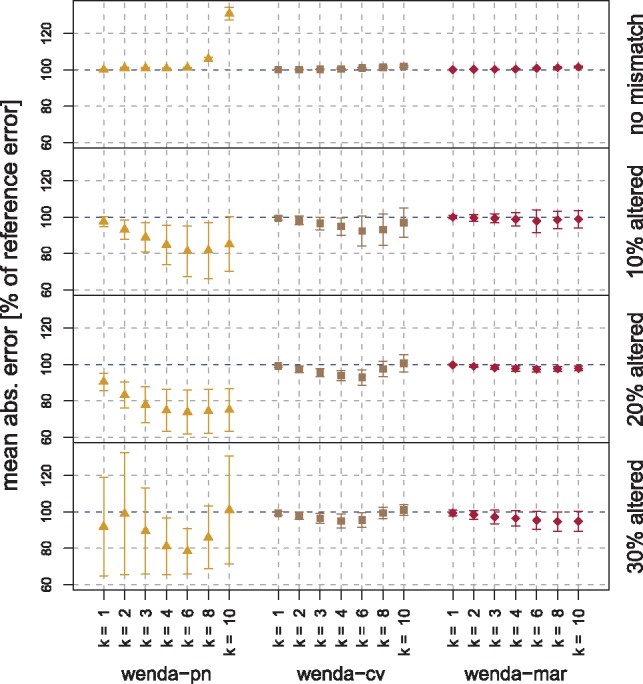
Mean absolute error (MAE) of wenda-pn, wenda-cv and wenda-mar on simulated test data. Each row shows results on one target domain (no mismatch, 10–30% altered variables). We report all errors relative to the MAE of en showing the mean±standard deviation over 10 simulations
With wenda-pn we obtain considerable improvements for the intermediate target domains with 10% and 20% altered variables, reducing the MAE of en by up to 18.7% and 26.2%, respectively. For the more extreme target domains the results are mixed. With 30% altered variables we still observe an improvement for some values of k, but the variability is very high (both within one choice and between choices of k). For the target domain without mismatch, the MAE even increases compared with en for high values of k. This can be explained by the cross-validation scheme we employ to learn the relationship between and domain similarity (Section 3.3). For each size of distribution mismatch, the model describing this relationship has been trained on the remaining target domains. This is an interpolation for the intermediate target domains (10% and 20% altered variables), but an extrapolation for the target domains with 30% altered variables and no mismatch. Extrapolation is a harder problem and can lead to a less accurate estimate of and increased variability.
It should be noted that using domain adaptation even though prior knowledge suggests that there is no distribution mismatch between domains is not a realistic scenario. We include the results of wenda-pn on data without distribution mismatch for the sake of completeness.
The other two weighted models, wenda-cv and wenda-mar show no or only very little improvement over en. On target domains with mismatch, wenda-cv consistently receives a slightly lower MAE than en, but the improvement is only 7.6% at best. It uses the same feature weights as wenda-pn, but obviously chooses a less suitable value for λ. The simpler confidences used by wenda-mar can only pick up changes in the marginal distributions of features, not in their dependency structure, leading to almost the same results as en. Only for 30% altered variables a slight improvement can be noted. Since marginal distributions are only altered very subtly in the target domain model, we expected a weak performance of wenda-mar in this simulation study.
4 Age prediction from DNA methylation data
Now we consider our primary application on real data, i.e. the problem of age prediction from DNA methylation data across multiple tissues.
4.1 DNA methylation dataset and preprocessing
We use DNA methylation data and donor age from two sources, the Cancer Genome Atlas (TCGA; Chang et al., 2013) and the Gene Expression Omnibus (GEO; Edgar et al., 2002). We include only DNA methylation data which were measured with the Illumina Infinium HumanMethylation450 BeadChip and only samples from healthy tissue. Using RnBeads (Assenov et al., 2014), we perform several preprocessing steps on the DNA methylation data. In particular, we remove SNPs and gonosomal CpGs, and normalize the data with the BMIQ method (Teschendorff et al., 2013b). In addition, we impute missing values (<0.5% of all measurements) using 10-nearest-neighbor imputation in the R package impute (Hastie et al., 2017). Finally, we split the dataset into a training and test set with 1866 and 1001 samples, respectively.
The final training set contains data from 19 different tissues, with a focus on blood, and from donors with a chronological age ranging from 0 to 103 years. The test set consists of data from 13 different tissues initially, including blood as well as tissues which are not present in the training data, e.g. samples from the cerebellum of the human brain. We slightly aggregate them, combining ‘blood’, ‘whole blood’ and ‘menstrual blood’, as well as ‘Brain MedialFrontalCortex’ and ‘Brain FrontalCortex’ to increase sample sizes per tissue. The range of ages represented in the test set is 0–70 years. When applying wenda, we keep the training set fixed and consider each tissue in the test set as a separate target domain.
To limit the computational burden of training feature models, we reduce the initial number of 466 094 features to 12 980 using a standard elastic net model with and fixed regularization parameter, λ=1.1 × 10⁻⁴. Furthermore, we use the following transformation for the chronological ages, which was proposed by Horvath (2013). We transform all training ages with the function
with adult age prior to training, and later re-transform the model’s predictions with the inverse function, . This transformation is logarithmic for ages below and linear for ages above , which is motivated by the fact that the methylation landscape changes more quickly and dramatically in childhood and adolescence than later in life. Subsequently, we standardize all data to zero mean and unit variance.
4.2 Prior knowledge on domain mismatch
As prior knowledge for wenda-pn (Section 2.5), we make use of published data on similarities between human tissues. The GTEx consortium published an analysis of a large dataset of (among others) genotype and gene expression data across 42 human tissues (Aguet et al., 2017). In this article, Aguet et al. (2017) identified tissue-specific expression quantitative trait loci (eQTLs), i.e. locations in the genome where genetic variants have a significant effect on gene expression levels. Furthermore, the authors estimated tissue-specific effect sizes for each eQTL using a linear mixed model, and reported the correlation (Spearman’s ρ) of effect sizes between all pairs of tissues (see Figure 2a in Aguet et al., 2017), providing a comprehensive measure of tissue similarity. Here we focus on the correlations reported for cis-eQTLs, where the location of the genetic variation is within 1 Mb of the target gene’s transcription start site, since these were identified in larger numbers and with a lower false discovery rate than trans-eQTLs.
Fig. 2.

(a) Mean absolute error of en-ls and wenda-pn with k = 3 per test tissue. We show the mean ± standard deviation over 10 runs of 10-fold cross-validation for en-ls, and over all splits of the test tissues where the tissue of interest was in the evaluation set for wenda-pn. Predicted versus true chronological age for typical runs of en-ls (b) and wenda-pn with k = 3 (c). In each plot, we show samples colored by tissue. As a typical run for en-ls we show the one with closest to median performance on cerebellum samples and full test set. For wenda-pn, we choose a typical run for each tissue: among all models with this tissue in the holdout set, we plot predictions of the one with closest to median performance
We map each tissue in our data to the corresponding tissue(s) contained in the GTEx study, allowing multiple matches if the GTEx classification is more detailed than the one available for our data (Supplementary Table S1). Next, we compute similarities between tissues in our data by looking up (and potentially averaging) the similarities between matched GTEx tissues. Finally, we define the similarity between each target domain and the source domain as the average over all pairwise similarities between samples from the two sets. Our data contains several samples from tissues for which no close match is available in the GTEx data (240 samples in the training set, 56 in the test set). For these we impute the similarity to other tissues with the mean of all pairwise tissue similarities.
When evaluating the performance of wenda-pn, we repeatedly split the test tissues into one part for fitting the relationship between domain similarity and and one part for evaluation (Section 2.5). Here, we iterate over all combinations of 3 tissues with at least 20 samples each for training and evaluate the performance on the remaining tissues.
4.3 Baseline models
We compare wenda-pn and wenda-cv to the two baseline models described in Section 3.4 with the following minor modification: instead of using a simple elastic net directly, we use en followed by a linear least-squares fit based only on features which received nonzero coefficients in en. We refer to this baseline as en-ls. This model type was suggested by Horvath (2013) for age prediction from DNA methylation data, who reported that the subsequent least-squares fit reduced test errors on his dataset. We observe a similar effect on our data, where en-ls produces lower test errors than en on cerebellum samples while making almost no difference on the remaining samples.
4.4 Results on DNA methylation data
We compare the results of wenda-pn, wenda-cv and the two baseline models on the dataset described in Section 4.1 and measure performance by MAE on the test set (Supplementary Figure S4 for correlation instead of MAE). Due to the heterogeneous nature of the data, the random split of the training data used for 10-fold cross-validation has a large influence on the results, especially for en-ls. Hence, we report the mean and standard deviation over 10 runs. For wenda-pn, we do not perform cross-validation on the training data but iterate over multiple splits of the test tissues to learn the relationship between domain similarity and . Here, we measure MAE only on samples which were not used for the similarity-lambda fit, and report mean and standard deviation over all splits.
When training the weighted models, we regard each tissue in the test dataset as a separate target domain. To be precise, we average the confidences defined in Equation (5) only over samples of the same tissue and train a separate model for each tissue, using always the same training data but tissue-specific feature weights.
With en-ls we obtain an MAE of 6.19 ± 0.90 years on the full test set. Figure 2a illustrates the MAE of en-ls and a representative example of a weighted model (wenda-pn, k = 3) on each test tissue. It shows that en-ls yields a considerably higher MAE on cerebellum samples than on other tissues. Figure 2b shows the predicted versus true ages for the test set in a typical cross-validation run, colored by tissue, and reveals that the predicted age is consistently far below the true chronological age. Both plots demonstrate that en-ls predicts age well on all test tissues except cerebellum. In fact, on cerebellum samples en-ls produces an MAE of 18.75 ± 7.18 years.
Cerebellum samples are especially hard to predict for two reasons: they are not represented in the training data and they are known to be biologically very different even from other brain tissues regarding function and gene expression patterns (Aguet et al., 2017; Fraser et al., 2005). Therefore, the focus of our evaluation is whether domain adaptation as implemented by wenda can improve performance on these samples.
The predictions of wenda-pn with k = 3 versus the true ages are shown in Figure 2c. Here, we plot the predictions of a typical run for each tissue by choosing the model with closest to median performance among all models with this tissue in the holdout set. The ages predicted by wenda-pn for cerebellum samples are far closer to the corresponding true ages than they were for en-ls (Fig. 2b), and predictions of wenda-pn on the remaining test tissues are of a similar quality as those of en-ls. This observation is confirmed by the quantitative comparison in Figure 2a, where wenda-pn has far lower errors than en-ls on cerebellum samples, and similar or better performance than en-ls on the remaining test tissues.
While en-ls predicts age far worse on cerebellum samples than on other tissues, wenda-pn shows no major difference in prediction quality between cerebellum samples and the remaining test tissues. Consequently, wenda-pn demonstrates to be considerably more robust to the distribution mismatch between cerebellum samples and the training data than en-ls.
Figure 3 shows the MAE of all models on cerebellum samples. Here, all weighted models strongly improve upon en-ls. The lowest errors on cerebellum samples are achieved by wenda-cv, reaching as low as 6.07 ± 0.10 years for k = 4. This is closely followed by wenda-pn, which achieves an MAE between 7.60 and 8.70 years on average on cerebellum samples for . Even wenda-mar, which uses only marginal distributions to weight features, improves upon en-ls with an MAE of 9.42 ± 0.69 years at best. All weighted models achieve their best result for k between 2 and 4 with not too much variation in this range. However, even when k is far from optimal for cerebellum samples, they still perform better than en-ls.
Fig. 3.
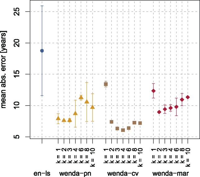
Mean absolute error of all models on cerebellum samples. We show the mean and standard deviation over 10 runs of 10-fold cross-validation or, in case of wenda-pn, over all splits where cerebellum samples were in the evaluation set
A comparison of the MAE of all models on the full test set is shown in Figure 4 and indicates an overall similar performance of wenda and the two baselines. For , wenda-cv and wenda-mar yield a slightly lower MAE than en-ls, and for large k, wenda-cv and wenda-pn yield a slightly higher MAE than en-ls. Given that en-ls already shows acceptable performance on all tissues except cerebellum, we did not expect a big improvement here. The results show, however, that the improvement on cerebellum samples is not bought by a loss of performance on other tissues.
Fig. 4.
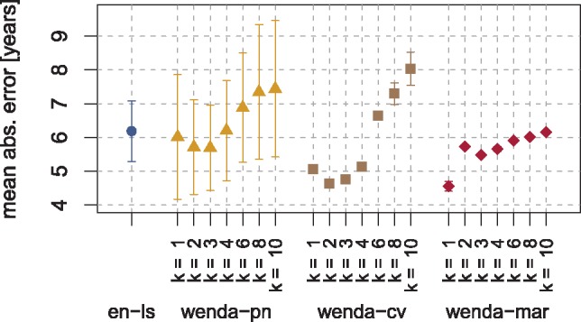
Mean absolute error (MAE) of all models on the full test set of DNA methylation data. We show the mean and standard deviation over 10 runs of 10-fold cross-validation. In case of wenda-pn, we compute the MAE only based on samples in the evaluation set, and plot the mean and standard deviation over all considered splits of the test tissues
5 Discussion
Predictive models are widely used in computational biology, but differences between the distribution of their training data and new data to which they are later applied can severely threaten their performance. In this article we propose wenda, a method for unsupervised domain adaptation based on the elastic net. It detects differences in the dependency structure between inputs in source and target domain and enforces stronger regularization on features that behave differently. Our method is different from previous studies on the combination of the elastic net and domain adaptation techniques (Li et al., 2015; Wachinger and Reuter, 2016). Both consider only the easier problem of supervised domain adaptation, i.e. the situation where some labeled examples from the target domain are available for training, and are not applicable in the setting we consider. Our method is also different from the approach proposed by Cortes and Mohri (2011), which uses a sample weighting rather than a feature weighting and is thus better suited for situations with n > p than for the ones we consider.
The key idea of our approach, which separates it from many other domain adaptation methods, is to learn the dependency structure between inputs for calculating feature weights. This property is of particular relevance to applications within computational biology where, in contrast to, e.g. image analysis, the dependency structure is irregular and not known a priori. For example, even distant locations in the (epi)genome can interact and form complex gene regulatory networks, which vary with cell type and differentiation state (Thompson et al., 2015). While we used Gaussian process models with linear kernels as feature models, any other Bayesian model type would be applicable in principle, subject only to the data and computational resources.
Like any domain adaptation method, wenda makes the assumption that source and target distribution are not too far apart, so that some features are useful for predicting the output and behave similarly in source and target domain. Another central assumption of our method is that the dependency structure between inputs is informative of which features are useful for domain adaptation. There are certain extreme cases, where this is clearly violated. For example, when features are entirely independent, the distribution predicted by each feature model gf would be approximately the feature’s marginal distribution, and wenda-pn and wenda-cv would behave similarly to wenda-mar. Another such case is the presence of duplicates or extremely strong correlations between variables. These could arise, e.g. in sequencing-based methylation assays, where the DNA methylation of consecutive CpG sites is highly correlated in all tissues. Thus, each feature would always be well predicted by its neighbor, regardless of changes on a larger scale. In situations like this, we suggest to aggregate extremely correlated features before training, which is also advisable for a standard elastic net.
Our method is computationally demanding since it requires to train one Bayesian model per feature (for confidence estimation) and one weighted elastic net per target domain (for prediction). While both of these steps can be parallelized to speed up calculations, fitting the feature models remains challenging for large datasets. For example, training 12 980 feature models for the DNA methylation data on 10 CPUs of the type Intel Xeon CPU E7-4850 with 2.30 GHz takes about 51 h.
However, the structure of wenda allows additional speed-ups, as feature models have to be trained only once (as long as the training data remain fixed) and can be reused to predict on multiple target domains or with different parameter settings. If the confidence scores for a given test dataset are precomputed as well, the final model for one target domain is only a weighted elastic net trained on the training data, whose regularization path can be computed quickly, e.g. with glmnet. With the same computational setup as before and with precomputed feature models and confidence scores, training all models required for wenda-pn with k = 3 (Fig. 2c) takes about 43 s.
Wenda allows to incorporate prior knowledge on the size of the domain mismatch (wenda-pn), but a simplified version can also be applied without it (wenda-cv). Wenda-cv uses cross-validation on the training data to determine λ, which is not ideal in a domain adaptation setting. Nevertheless, our results on the DNA methylation data demonstrate that it can still lead to a surprisingly large improvement over a non-adaptive model. This makes it a valuable alternative to wenda-pn, especially if no prior knowledge on the size of domain mismatch is available.
Wenda introduces a new parameter k, which controls how confidences are translated into feature weights. We empirically studied the impact of choosing k on the MAE and observed satisfying performance in the interval . Hence, k = 3 might constitute a relatively robust choice for future applications, albeit it is unlikely that any single parameter choice is optimal for each and every target domain. We note that wenda never performs substantially worse than the non-adaptive reference. Hence, the precise value of k determines only the magnitude of improvement obtained and a suboptimal choice poses relatively little risk. Nevertheless, without labeled training examples from the target domain, parameter selection remains a non-trivial problem. Finding a data-driven way to determine an optimal choice for k, or evaluating whether α can be optimized additionally, are challenging themes for future research.
6 Conclusions
In this article we propose wenda, a method for unsupervised domain adaptation which is based on the elastic net and utilizes dependencies between inputs to detect differences between source and target domain. Using a weighted elastic net penalty, wenda enforces stronger regularization on features that behave differently in the two domains, reducing the effects of a distribution mismatch.
We compare two variants of our method, wenda-pn and wenda-cv, on simulated datasets and on real data, where we considered the problem of age prediction from DNA methylation data across tissues. Our experimental results demonstrate that both variants can reduce test errors on samples with a distribution mismatch. While wenda-cv outperforms the non-adaptive reference only on real data, wenda-pn strongly reduces errors on test samples with a distribution mismatch both on real and simulated data, which makes it the more promising variant for future applications.
From a wider perspective, this article demonstrates that the ambitious goal of unsupervised domain adaptation is indeed feasible not only for big data analysis with deep learning methods, but also for traditional machine learning methods that are useful for analyzing relatively small datasets as they frequently occur in computational biology and medicine.
Supplementary Material
Acknowledgements
We would like to thank Dr Alexis Battle and Ben Strober for kindly providing the matrix of similarities plotted in Figure 2a in Aguet et al. (2017). We additionally thank Martina Feierabend for reviewing the mapping of tissues between their data and ours.
Funding
This work was prepared within the project XplOit of the initiative ‘i: DSem—Integrative Datensemantik in der Systemmedizin’, funded by the German Federal Ministry of Education and Research (BMBF).
Conflict of Interest: none declared.
References
- Aguet F. et al. (2017) Genetic effects on gene expression across human tissues. Nature, 550, 204–213. [DOI] [PMC free article] [PubMed] [Google Scholar]
- Akey J.M. et al. (2007) On the design and analysis of gene expression studies in human populations. Nat. Genet., 39, 807–808. [DOI] [PubMed] [Google Scholar]
- Aljundi R. et al. (2015) Landmarks-based kernelized subspace alignment for unsupervised domain adaptation. In: Proceedings of the 2015 IEEE Conference on Computer Vision and Pattern Recognition (CVPR), 2015: 8–10 June, 2015, pp. 56–63. Boston, Massachusetts, USA.
- Almagro Armenteros J.J. et al. (2017) DeepLoc: prediction of protein subcellular localization using deep learning. Bioinformatics, 33, 3387–3395. [DOI] [PubMed] [Google Scholar]
- Angermueller C. et al. (2017) DeepCpG: accurate prediction of single-cell DNA methylation states using deep learning. Genome Biol., 18, 67.. [DOI] [PMC free article] [PubMed] [Google Scholar]
- Assenov Y. et al. (2014) Comprehensive analysis of DNA methylation data with RnBeads. Nat. Methods, 11, 1138–1140. [DOI] [PMC free article] [PubMed] [Google Scholar]
- Bell J.T. et al. (2012) Epigenome-wide scans identify differentially methylated regions for age and age-related phenotypes in a healthy ageing population. PLOS Genet., 8, e1002629.. [DOI] [PMC free article] [PubMed] [Google Scholar]
- Chang K. et al. (2013) The cancer genome atlas pan-cancer analysis project. Nat. Genet., 45, 1113–1120. [DOI] [PMC free article] [PubMed] [Google Scholar]
- Christensen B.C. et al. (2009) Aging and environmental exposures alter tissue-specific DNA methylation dependent upon CpG island context. PLOS Genet., 5, e1000602.. [DOI] [PMC free article] [PubMed] [Google Scholar]
- Civis Analytics (since 2016) python-glmnet: A Python Port of the glmnet Package for Fitting Generalized Linear Models via Penalized Maximum Likelihood. Python Package Version 2.0.0. http://github.com/civisanalytics/python-glmnet (10 May 2019, date last accessed)
- Cortes C., Mohri M. (2011) Domain adaptation in regression. In: Proceedings of the 2011 International Conference on Algorithmic Learning Theory (ALT), 5–7 October, 2011, pp. 308–323. Espoo, Finland.
- Day K. et al. (2013) Differential DNA methylation with age displays both common and dynamic features across human tissues that are influenced by CpG landscape. Genome Biol., 14, R102.. [DOI] [PMC free article] [PubMed] [Google Scholar]
- Edgar R. et al. (2002) Gene expression omnibus: NCBI gene expression and hybridization array data repository. Nucleic Acids Res., 30, 207–210. [DOI] [PMC free article] [PubMed] [Google Scholar]
- Farh K.K.-H. et al. (2015) Genetic and epigenetic fine mapping of causal autoimmune disease variants. Nature, 518, 337–343. [DOI] [PMC free article] [PubMed] [Google Scholar]
- Florath I. et al. (2014) Cross-sectional and longitudinal changes in DNA methylation with age: an epigenome-wide analysis revealing over 60 novel age-associated CpG sites. Hum. Mol. Genet., 23, 1186–1201. [DOI] [PMC free article] [PubMed] [Google Scholar]
- Fraser H.B. et al. (2005) Aging and gene expression in the primate brain. PLOS Biol., 3, e274.. [DOI] [PMC free article] [PubMed] [Google Scholar]
- Friedman J. et al. (2010) Regularization paths for generalized linear models via coordinate descent. J. Stat. Softw., 33, 1–22. [PMC free article] [PubMed] [Google Scholar]
- Ganin Y. et al. (2016) Domain-adversarial training of neural networks. J. Mach. Learn. Res., 17, 1–35. [Google Scholar]
- Garnett M.J. et al. (2012) Systematic identification of genomic markers of drug sensitivity in cancer cells. Nature, 483, 570–575. [DOI] [PMC free article] [PubMed] [Google Scholar]
- Gong B. et al. (2012) Geodesic flow kernel for unsupervised domain adaptation. In: Proceedings of the 2012 IEEE Conference on Computer Vision and Pattern Recognition (CVPR), 16–21 June, 2012, pp. 2066–2073. Rhode Island, USA.
- Gong B. et al. (2013) Connecting the dots with landmarks: discriminatively learning domain-invariant features for unsupervised domain adaptation. In: Proceedings of the 30th International Conference on Machine Learning (ICML), 16–21 June, 2013, pp. 222–230. Atlanta, Georgia, USA.
- GPy (since 2012) GPy: A Gaussian Process Framework in Python Python Package Version 1.5.3. http://github.com/SheffieldML/GPy (10 May 2019, date last accessed).
- Hannum G. et al. (2013) Genome-wide methylation profiles reveal quantitative views of human aging rates. Mol. Cell, 49, 359–367. [DOI] [PMC free article] [PubMed] [Google Scholar]
- Hastie T. et al. (2017) impute: Imputation for Microarray Data R Package Version 1.52.0. http://www.bioconductor.org/packages/release/bioc/html/impute.html (10 May 2019, date last accessed).
- Heyn H. et al. (2012) Distinct DNA methylomes of newborns and centenarians. Proc. Natl. Acad. Sci. U.S.A., 109, 10522–10527. [DOI] [PMC free article] [PubMed] [Google Scholar]
- Hoerl A.E., Kennard R.W. (1970) Ridge regression: biased estimation for nonorthogonal problems. Technometrics, 12, 55–67. [Google Scholar]
- Hoiles W., van der Schaar M. (2016) A non-parametric learning method for confidently estimating patient’s clinical state and dynamics. Adv. Neural Inform. Process. Syst., 29, 2020–2028. [Google Scholar]
- Horvath S. (2013) DNA methylation age of human tissues and cell types. Genome Biol., 14, R115.. [DOI] [PMC free article] [PubMed] [Google Scholar]
- Hughey J.J., Butte A.J. (2015) Robust meta-analysis of gene expression using the elastic net. Nucleic Acids Res., 43, e79.. [DOI] [PMC free article] [PubMed] [Google Scholar]
- Ide J.S., Cozman F.G. (2002) Random generation of Bayesian networks. In: Advances in Artificial Intelligence, Lecture Notes in Computer Science, Springer, Berlin.
- Jalali A., Pfeifer N. (2016) Interpretable per case weighted ensemble method for cancer associations. BMC Genom., 17, 501. [DOI] [PMC free article] [PubMed] [Google Scholar]
- Jansen R. et al. (2003) A Bayesian networks approach for predicting protein-protein interactions from genomic data. Science, 302, 449–453. [DOI] [PubMed] [Google Scholar]
- Krogan N.J. et al. (2006) Global landscape of protein complexes in the yeast Saccharomyces cerevisiae. Nature, 440, 637–643. [DOI] [PubMed] [Google Scholar]
- Leek J.T. et al. (2010) Tackling the widespread and critical impact of batch effects in high-throughput data. Nat. Rev. Genet., 11, 733–739. [DOI] [PMC free article] [PubMed] [Google Scholar]
- Leffler E.M. et al. (2017) Resistance to malaria through structural variation of red blood cell invasion receptors. Science, 356, eaam6393.. [DOI] [PMC free article] [PubMed] [Google Scholar]
- Lengauer T., Sing T. (2006) Bioinformatics-assisted anti-HIV therapy. Nat. Rev. Microbiol., 4, 790–797. [DOI] [PubMed] [Google Scholar]
- Li Y. et al. (2015) Constrained elastic net based knowledge transfer for healthcare information exchange. Data Min. Knowl. Discov., 29, 1094–1112. [Google Scholar]
- Long M. et al. (2016) Unsupervised domain adaptation with residual transfer networks. Adv. Neural Inform. Process. Syst., 29, 136–144. [Google Scholar]
- Margolis A. (2011) A Literature Review of Domain Adaptation with Unlabeled Data. Technical Report, University of Washington.
- Pan S.J., Yang Q. (2010) A survey on transfer learning. IEEE Trans. Knowl. Data Eng., 22, 1345–1359. [Google Scholar]
- Patel V.M. et al. (2015) Visual domain adaptation: a survey of recent advances. IEEE Signal Process. Mag., 32, 53–69. [Google Scholar]
- Pearl J. (1988) Probabilistic Reasoning in Intelligent Systems: Networks of Plausible Inference. Morgan Kaufmann Publishers Inc, San Francisco. [Google Scholar]
- Rasmussen C.E., Williams C.K.I. (2006) Gaussian Processes for Machine Learning. MIT Press, Cambridge, MA. [Google Scholar]
- Saito T., Sætrom P. (2012) Target gene expression levels and competition between transfected and endogenous microRNAs are strong confounding factors in microRNA high-throughput experiments. Silence, 3, 3.. [DOI] [PMC free article] [PubMed] [Google Scholar]
- Schmidt F. et al. (2017) Combining transcription factor binding affinities with open-chromatin data for accurate gene expression prediction. Nucleic Acids Res., 45, 54–66. [DOI] [PMC free article] [PubMed] [Google Scholar]
- Schübeler D. (2015) Function and information content of DNA methylation. Nature, 517, 321–326. [DOI] [PubMed] [Google Scholar]
- Stranger B.E. et al. (2011) Progress and promise of genome-wide association studies for human complex trait genetics. Genetics, 187, 367–383. [DOI] [PMC free article] [PubMed] [Google Scholar]
- Teschendorff A.E. et al. (2013) Age-associated epigenetic drift: implications, and a case of epigenetic thrift? Hum. Mol. Genet., 22, R7–R15. [DOI] [PMC free article] [PubMed] [Google Scholar]
- Teschendorff A.E. et al. (2013) A beta-mixture quantile normalization method for correcting probe design bias in Illumina Infinium 450 k DNA methylation data. Bioinformatics, 29, 189–196. [DOI] [PMC free article] [PubMed] [Google Scholar]
- Thompson D. et al. (2015) Comparative analysis of gene regulatory networks: from network reconstruction to evolution. Annu. Rev. Cell Dev. Biol., 31, 399–428. [DOI] [PubMed] [Google Scholar]
- Tibshirani R. (1996) Regression shrinkage and selection via the lasso. J. Royal Stat. Soc. Ser. B (Stat. Methodol.), 58, 267–288. [Google Scholar]
- Varley K.E. et al. (2013) Dynamic DNA methylation across diverse human cell lines and tissues. Genome Res., 23, 555–567. [DOI] [PMC free article] [PubMed] [Google Scholar]
- Wachinger C., Reuter M. (2016) Domain adaptation for Alzheimer’s disease diagnostics. NeuroImage, 139, 470–479. [DOI] [PMC free article] [PubMed] [Google Scholar]
- Zhu T. et al. (2018) Cell and tissue type independent age-associated DNA methylation changes are not rare but common. Aging, 10, 3541–3557. [DOI] [PMC free article] [PubMed] [Google Scholar]
- Ziller M.J. et al. (2013) Charting a dynamic DNA methylation landscape of the human genome. Nature, 500, 477–481. [DOI] [PMC free article] [PubMed] [Google Scholar]
- Zou H., Hastie T. (2005) Regularization and variable selection via the elastic net. J. Royal Stat. Soc. Ser. B (Stat. Methodol.), 67, 301–320. [Google Scholar]
Associated Data
This section collects any data citations, data availability statements, or supplementary materials included in this article.