Muscle Segmentation in axial Computed Tomography (CT) Images at the Lumbar (L3) and Thoracic (T4) levels for Body Composition Analysis

Abstract

In diseases such as cancer, patients suffer from degenerative loss of skeletal muscle (cachexia). Muscle wasting and loss of muscle function/performance (sarcopenia) can also occur during advanced aging. Assessing skeletal muscle mass in sarcopenia and cachexia is therefore of clinical interest for risk stratification. In comparison with fat, body fluids and bone, quantifying the skeletal muscle mass is more challenging. Computed tomography (CT) is one of the gold standard techniques for cancer diagnostics and analysis of progression, and therefore a valuable source of imaging for in vivo quantification of skeletal muscle mass. In this paper, we design a novel deep neural network-based algorithm for the automated segmentation of skeletal muscle in axial CT images at the third lumbar (L3) and the fourth thoracic (T4) levels. A two-branch network with two training steps is investigated. The network’s performance is evaluated for three trained models on separate datasets. These datasets were generated by different CT devices and data acquisition settings. To ensure the model’s robustness, each trained model was tested on all three available test sets. Errors and the effect of labeling protocol in these cases were analyzed and reported. The best performance of the proposed algorithm was achieved on 1327 L3 test samples with an overlap Jaccard score of 98% and sensitivity and specificity greater than 99%.

1. Introduction

Measuring skeletal muscle mass is essential in many clinical conditions. Cross-sectional areas at the third lumbar vertebral level (L3) are considered to be linearly related to the whole body muscle mass (Shen et al., 2004; Mourtzakis et al., 2008). The thoracic muscle cross sectional area from a single axial slice at the fourth thoracic (T4) to sixth thoracic (T6) is also correlated with the measure of muscle volume (Mathur et al., 2017). Conventionally, the segmentation is anatomic and is done by someone trained in anatomical radiology and the Hounsfield unit (HU) is used as a secondary element for segmenting skeletal muscle, adipose tissue, and bone on computed tomography (CT) images. The standard Hounsfield unit (HU) for skeletal muscle has overlapping values with HU of neighboring organs. Therefore, a segmentation based on thresholding with this range of values still needs manual correction. This leads to a time consuming and expensive overall process hence motivating the need for developing automated segmentation algorithms.

Muscle segmentation in L3 (Chung et al., 2009; Popuri et al., 2016) and in T4 (Popuri et al., 2013) using a shape prior modeling approach has been previously reported. Kamiya et al. addressed the segmentation of individual muscle groups such as psoas major and rectus abdominis muscles from CT images by generating muscle group specific shape models (Kamiya et al., 2009; Kamiya et al., 2012). Another model-based approach for psoas major segmentation in CT images has been proposed in (Meesters et al., 2012) using a multi-atlas fusion based segmentation framework. Paraspinal muscle segmentation using fuzzy c-means clustering algorithm has been explored in (Wei et al., 2014). Finding the optimal features has always been a crucial step in automatic segmentation and design of hand-crafted features for model-based techniques. However, with deep neural networks, this step is eliminated as the network itself finds the most discriminant features based on the training ground truth labels and the chosen objective function.

Previous work on applying deep learning on segmentation of L3 CT images is limited. A convolutional neural network (CNN) (Goodfellow et al., 2016) approach for this specific task of skeletal muscle segmentation is a fully convolutional network (FCN) method (Lee et al., 2017). The structure of FCN is a popular network among semantic segmentation architectures, but it has limitations such as the spatial resolution reduction on final prediction. Despite the connections between decoder and encoder layers and merging the predictions from different pooling layers in the model suggested by Long et al. (Long et al., 2015), there is still some loss of spatial information in the final prediction. Other recent publications have used CNN for segmentation of brain regions and tumor segmentation (Pereira et al., 2016; Havaei et al., 2017; Moeskops et al., 2016; Zhang et al., 2015; De Brébisson and Montana, 2015). CNNs were also used on CT images as for example pancreas segmentation in CT images (Roth et al., 2015), knee cartilage segmentation (Prasoon et al., 2013) and cardiac CT angiography (Wolterink et al., 2016).

In this paper, a novel deep neural network-based algorithm is proposed for automatic segmentation of muscle tissue in abdominal and thoracic CT images. The main elements that were considered in this architecture were aligned to our goals of 1) keeping dense and fine information of the input image, and 2) reducing the generalization error. To achieve the first point, we benefited from two powerful existing architectures, the fully convolutional network (FCN) (Long et al., 2015) and the UNet (Ronneberger et al., 2015). Our second important objective was to reduce the generalization error. Most of the networks proposed for a specific medical image modality are not broad enough to include other sets of data from other devices with different data acquisition settings. In order to overcome this problem, different generalization methods like the pooling layers, data augmentation, and early stopping were applied and investigated on three different datasets.

2. Methods

2.1. CT data variability

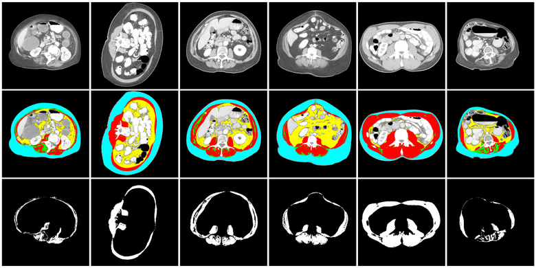
The novel deep neural network-based segmentation algorithm proposed in this manuscript is designed for muscle segmentation on L3 and T4 axial slices taken from CT images. A normal L3 axial slice taken from a CT image comprises four major compartments namely skeletal muscle (SM), visceral adipose tissue (VAT), subcutaneous adipose tissue (SAT) and inter-muscular adipose tissue (IMAT) as shown in representative images from several individuals in Figure 1. The top row shows the raw CT L3 images, the middle row shows segmentation of the above-mentioned four regions in different colors and the bottom row shows the skeletal muscle outline only highlighting the challenge of considerable variability observed across individuals.

Figure 1:

Illustration of variation of tissue types, specifically skeletal muscle tissue, in the dataset. Top row shows a CT image axial slice centered on the third lumbar vertebra (L3). In the middle row, the images corresponding to skeletal muscle (SM, red), vascular adipose tissue (VAT, yellow), subcutaneous adipose tissue (SAT, blue) and inter-muscular adipose tissue (IMAT, green) segments are illustrated. The bottom row shows the manual segmentations (taken as ground truth) for skeletal muscle tissue.

2.2. Dataset

Three datasets from L3 slices of CT scan and a single T4 CT dataset are used in this paper. The ethics approval for the study was provided by the institutional review board. The first database of L3 CT images were acquired at the Cross Cancer Institute (CCI), University of Alberta, Canada. This dataset consisted of 1075 abdominal and 709 thoracic axial CT images taken at the L3 and T4 level respectively from patients with head, neck and lung cancers. The abdominal images were obtained from 670 patients and the thoracic images were obtained from 334 patients. Manual segmentation of the muscle and fat regions were available for all the images in the Dataset-1. The manual segmentation was performed by a single expert operator using Slice-O-Matic V4.3 software (Tomovision, Montreal, Canada). 645 samples from Dataset-1 used for training the network and other 430 samples were used as the first test set.

Dataset-2 of L3 CT images comes from the ”C-scan Study” of patients diagnosed with stage IIII invasive colorectal cancer who had a surgical resection at Kaiser Permanente Northern California (KPNC) between 2006 and 2011 (Caan et al., 2017). Participants (male/female) were taken from range of race/ethnicity and body mass index (BMI) categories. A trained researcher quantified the muscle tissue discriminating components using Slice-O-Matic Software version 5.0. This dataset includes 5101 images, 3774 of which were used for training the network and the rest 1327 images used as the second test set.

Dataset-3 of L3 CT images is from female patients in the ”B-scan Study” aged 18 to 80 years diagnosed with stage II or III invasive breast cancer at KPNC between January 2005 and December 2013 (Caan et al., 2018). Two trained researchers quantified the cross-sectional area of muscle using Slice-O-Matic Software version 5.0. This dataset includes 3003 images, 1802 of which were used for training the network and the rest 1201 images used as the third test set.

2.3. Feature Learning

Deep convolutional neural networks learn the task specific features during the training process. The main elements of a CNN are convolution layers (LeCun et al., 1998). Each layer is trained (Rumelhart et al., 1986) to finally extract the relevant features.

An activation function is applied on the output feature map on each layer, to find the non-linear transformations. Rectified linear unit (Nair and Hinton, 2010) and sigmoid are two types of these activation functions that are employed in the proposed networks.

2.4. Network Architecture

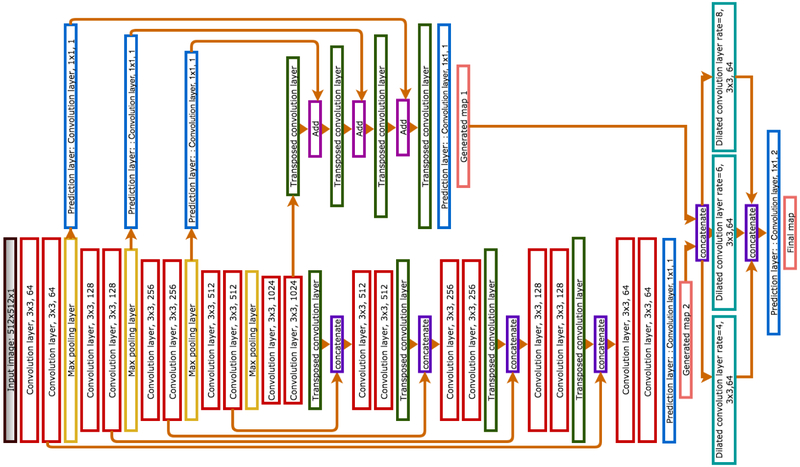
The proposed architecture is inspired by the FCN (Long et al., 2015) and the UNet (Ronneberger et al., 2015) models. The segmentation masks generated from these models showcase the strengths and weaknesses of these two architectures. The FCN estimates the coarse muscle tissue features, while the UNet shows better performance in extracting the finer boundaries at the expense of more false positive regions in some irrelevant places. The logic behind combining these two models into one architecture was to harness their individual strengths while mitigating their collective drawbacks. Figure 2 presents a schematic depiction of the model. The proposed architecture consists of three major parts and three predictions. While only the final prediction from the last layer is considered as the network’s predicted map, the two other predicted masks were used for computing the loss. These predictions are discussed in sections 2.4.1, 2.4.2 and 2.4.3. Figure 3 illustrates different layers and their details.

Figure 2:

Different steps of the proposed method are illustrated schematically. This model has three outputs, denoted as the first map, the second map and the final map (output).

Figure 3:

The proposed network architecture. Information flows from the left to the right of the network. Input image on the left is the gray scale CT slice and final map on the right is the segmentation mask. Colors of boxes indicate the type of layer in the network.

2.4.1. First prediction

The first prediction is the summation of predictions from pooling layers of the encoder. The encoder part of the network is a FCN. The architectures of FCN with VGG16 (Simonyan and Zisserman, 2014) blocks and different strides has been studied by Lee et al. (Lee et al., 2017), and the best results were found with stride-two model for muscle segmentation task. Based on the procedure for FCN with 16 pixel stride (Long et al., 2015), a convolution layer with 1 × 1 filter was added on top of all pooling layers. The prediction taken from the two pixel stride layer, is generated by summing the output of all pooling layers with the final output. This requires up-sampling for upper layers so that they reach the same size as the previous layer. Finally, to get the original image size the prediction was up-sampled once more.

2.4.2. Second prediction

Based on the fully convolutional encoder-decoder model (Ronneberger et al., 2015), the skip connection between encoder layers and decoder layers with the same level is an important feature of this architecture. These connections translate the spatial information on the earlier encoder layers to the decoder and result in fine boundaries in the generated mask.

The encoder blocks consist of two convolution layers with the same number of feature channels followed by a max-pooling layer. ReLu is the activation function of all convolution layers in this part of the network. The decoder blocks also consist of two convolution layer followed by a transpose convolution layer. Applying the transpose convolution layer, the feature maps from the previous layers in each step were up-sampled to reach the original input dimension.

2.4.3. Final prediction

In this part of the network the first two predictions were concatenated and were given as input to the three parallel dilated convolution layers with different rates. Dilated convolution is a convolution layer that can be used instead of pooling layer such that the receptive field is increased without increasing the parameters or reducing resolution (Yu and Koltun, 2015). The reason of employing dilated convolution in this architecture is the vast range of variation in the input data. Obesity and muscle wasting are two factors that can cause considerable variation in the size and thickness of the muscle tissue even in similar sex and age ranges. An automatic segmentation architecture robust to these variations and not restricted to a special group subjects is the goal.

2.5. Training

The proposed network is trained in two steps. First, the encoder-decoder part is trained on the training set and then the full network shown in Figure 3 is trained while the encoder-decoder layers are initialized by the trained model in the previous step. For the other layers, random initialization was considered. In Dataset-1 and Dataset-3, 60% of the data is used for training and the rest was segregated for testing. In Dataset-2, 80% of the total data is used for training and the rest for testing. In every training iteration, 20% of the training data is used for validation and hyper-parameter optimization ensuring a complete separation of the validation data from the testing data.

Encoder-decoder training.

Dice coefficient is a similarity measure that quantifies the similarity between two images. The loss function chosen for training is the negative of the Dice coefficient.

Full network training.

The full network’s loss function is the cross-entropy loss. The cross-entropy loss is calculated for first, second and final map prediction. Then the weighted summation of these three losses is the network’s total loss. The best performance was achieved while training the network with the loss weight vector of [0.2, 0.2, 1] for the first, second and final prediction map, respectively. The Adam optimizer was used in both steps of the training.

2.6. Experiments

2.6.1. Pre-processing

CT images are stored in DICOM format. The normal images’ sizes are 512 by 512. In this step the DICOM images are converted to grey scale PNG images. All images were standardized so that their pixel value lie in the range of [0,1].

2.6.2. Data augmentation

Data augmentation reduces the possibility of over-fitting and improves the generalization of the network. In data augmentation, the available training samples are modified and then added to the dataset. The pixel classes should be invariant to the transformations applied on the data. Random rotation, horizontal and vertical flip are the transformations used in this paper on the training dataset which increased the number of samples by 4. Augmentation is only done on the training set and not the validation data.

2.6.3. Implementation

Spatial pooling layer.

In order to keep the resolution and expand the receptive fields, dilated convolution is used in the last layer of the network. Since the goal is pixel wise segmentation, it is crucial to use techniques that preserve the resolution and learned features in the deeper layers of the network. Different dilation rates were applied on the input image of the spatial pooling layer, as the result three dilation rates of 4, 6 and 8 with the filter size of 3 × 3 form the spatial pooling layer.

Early stopping.

In addition to data augmentation, early stopping was added to our training process as another factor to reduce generalization error. In early stopping, the number of training epochs is considered as a hyperparameter which is related to the validation loss. In this process, the validation loss is monitored and the model with the lowest validation loss is stored. After each update on the best model, the network continues training for another limited number of iterations and if the validation loss does not improve, the training process terminates.

2.6.4. Post-processing

The skeletal muscle on CT images is found to range between [−29, 150] HU in intensity. This is used in the post processing steps to remove pixels that classified as muscle but are outside this intensity range.

2.6.5. T4 muscle segmentation

The T4 dataset includes 709 images. Since significantly more data from L3 datasets was available, transfer learning is applied for training the networks trained on L3 images for muscle segmentation at the T4 level. Transfer learning is based on the assumption that learned features from the training process for L3 muscle segmentation are relevant to the required features for T4 muscle segmentation. Therefore, fine-tuning the L3 trained model will help to generalize from only a few T4 samples. The trained network with Dataset-2 from the L3 datasets was fine-tuned, with a different ratio of samples of axial CT slices, on the T4 training set.

3. Results

A few representative images taken from different subjects shown in Figure 1 indicate the presence of a broad range of variations on the tissue composition in these images likely influenced by gender, age, weight and different diseases. In addition to these variations, different acquisition procedures at different imaging centers may also add to the observed variability. Training a generalized model that can perform well across the range of observed variations necessitates gathering a database that includes these variations or to generate data considering these parameters in the data augmentation step.

The generalization to unseen images was investigated by training the proposed network on each of the three datasets separately and using subsets of the three datasets set aside for testing. The samples in these three datasets are from both men and women with different BMI ranges, and were acquired by different devices taken from different centers/imaging protocols. The performance, summarized in Table 1 shows that the model trained on Dataset-2 has the highest Jaccard score when tested on Dataset-1 and Dataset-2. For Dataset-3, the best test performance was achieved from applying the model trained on Dataset-3 itself.

Table 1:

The quantitative results of the three trained model on three test sets of L3 images. The second, third and the fourth rows from the top are the results of applying each of the three networks on the test samples set aside for Dataset-1, Dataset-2 and Dataset-3.

Test set (Number of samples)	Training set (Number of samples)	Jaccard Score	Dice Coefficient	Sensitivity	Specificity
Dataset-1 (430)	Dataset-1 (645)	96.34 ± 2.77	98.11 ± 1.47	98.15 ± 1.63	99.81 ± 0.19
	Dataset-2 (3774)	97.42 ± 1.95	98.68 ± 1.02	98.73 ± 1.01	99.86 ± 0.14
	Dataset-3 (1802)	93.83 ± 2.93	96.79 ± 1.61	95.27 ± 1.72	99.84 ± 0.22
Dataset-2 (1327)	Dataset-1 (645)	96.83 ± 3.15	98.36 ± 1.76	98.24 ± 2.16	99.87 ± 0.16
	Dataset-2 (3774)	98.27 ± 1.88	99.12 ± 1	99.29 ± 0.94	99.90 ± 0.12
	Dataset-3 (1802)	94.47 ± 3.14	97.13 ± 1.79	95.37 ± 2.2	99.91 ± 0.15
Dataset-3 (1201)	Dataset-1 (645)	93.70 ± 3.22	96.70 ± 1.84	98.49 ± 1.99	99.62 ± 0.21
	Dataset-2 (3774)	94.78 ± 2.53	97.29 ± 1.39	99.26 ± 1.55	99.64 ± 0.18
	Dataset-3 (1802)	96.01 ± 2.39	97.94 ± 1.30	97.99 ± 1.31	99.84 ± 0.15

The best result observed is the mean Jaccard score of 98% along with over 99% Dice score, sensitivity and specificity that was achieved on 1327 L3 test samples showing very high performance on a significantly large number of images attesting to the robustness of this method. The reduction in performance in some cross-database experiments could be attributed to different manual labeling protocols followed for the datasets. Note that the test set is identical in bench marking the performance of the three separately trained networks, and some samples of segmented muscle maps for each of these three networks are shown in Figure 4.

Figure 4:

Illustration of performance on some samples from the three datasets with networks trained on the training images of the corresponding dataset. The top row shows some L3 samples. In the middle row, their corresponding manual muscle segmentations are illustrated. The bottom row shows the overlay of the prediction mask with the trained model and the ground truth. Yellow regions are the pixels that are correctly classified as muscle. Red pixels are the pixels that are mis-classified as muscle and green pixels are the muscle pixels which are missed from prediction. Note that the predicted automatic segmentation performs well on a range of muscle profiles.

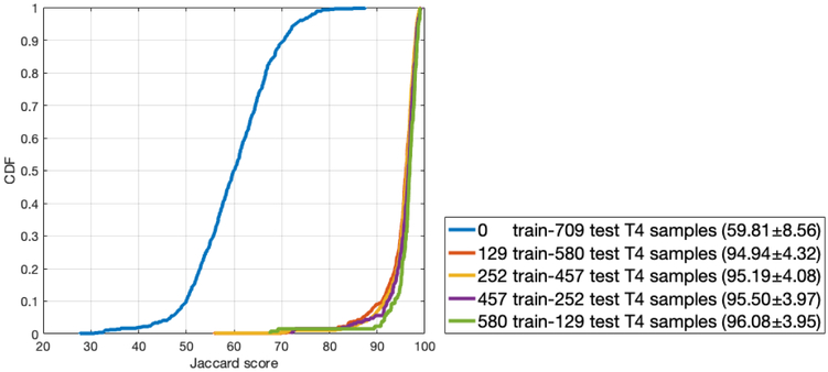
The model trained on L3 images from Dataset-2 was further used for fine-tuning the network to segment the muscle on CT images at the T4 level. Five experiments with various percentages of training and test samples were conducted and the results are presented in Figure 5. In this Figure, the blue line is the distribution of Jaccard scores on the whole dataset of T4 with the trained model using L3 vertebral level images from Dataset-2 with no further training on T4 vertebral level images. The other four curves are the distribution of Jaccard scores when the L3-based model from Dataset-2 was refined using different number of T4 images in each experiment and tested on the remainder. As the number of training samples increase (number of test samples decrease), the model performance also tends to increase although even with a few training samples, the model tends to perform well.

Figure 5:

The cumulative distribution function (CDF) plot of the Jaccard scores obtained from the experiments on T4 dataset to assess sensitivity to number of T4 images used for refining the network that was trained on L3 images from Dataset-2. The Jaccard scores (μ ± σ) for each experiment is presented in the box to the right of the graph.

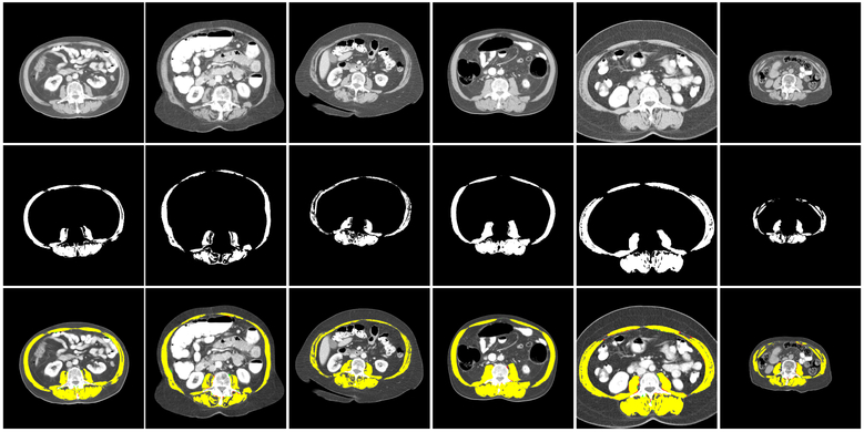
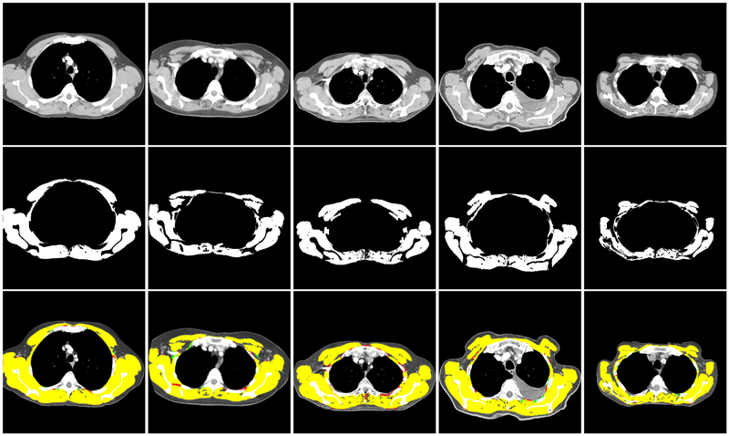
In Figure 6 some samples of the predicted segmentation mask from the model trained with approximately 80% of T4 dataset and tested on the remaining unseen 20% of the database are shown.

Figure 6:

Illustration of performance on the T4 dataset. Top row shows some T4 samples. In the middle row, their corresponding manual muscle segmentation are illustrated. Bottom row shows the overlaying result of the predicted map and ground truth. Yellow regions are the pixels that are correctly classified as muscle. Red pixels are the pixels that are mis-classified as muscle and green pixels are the muscle pixels which are missed from predicted map. Note that the predicted automatic segmentation performs well on a range of muscle profiles.

4. Discussion

We developed a deep neural network-based segmentation algorithm inspired by models presented in (Ronneberger et al., 2015) and (Long et al., 2015). Important criterion for us in developing this architecture were to retain high spatial resolution, the smoothness of labeling within a given region and the accuracy of the boundary for small degenerated areas in the muscle.

Analysis of performance on Dataset-1.

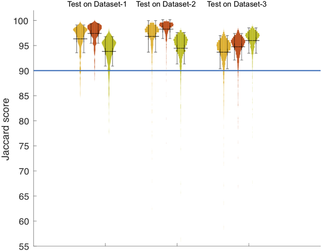
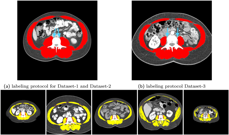
The top row of table 1 shows the quantitative results of applying the three models trained on Dataset-1, Dataset-2, and Dataset-3 to the unseen test set 1 from Dataset-1. The performance on this test set was similar across models trained on Dataset-1 and Dataset-2 but slightly higher from the model trained on Dataset-2. Since Dataset-1 and Dataset-2 have the same labeling protocol, the model trained with a higher number of samples likely led to the observed better test results. Figure 7 illustrates the distribution of Jaccard overlap scores for each experiment as a histogram on the vertical axis. The three first graph on the left refers to the models’ performance on Dataset-1. Based on this plot, each sample in test set 1 has a Jaccard score above 0.84 irrespective of the applied training model. Moreover, this graph suggests that while the trained model on Dataset-1 and the trained model on Dataset-2 have the same behaviour, the trained model on Dataset-3 has different distribution. This observation is also associated with the fact that Dataset-3 has a different labeling protocol. The key difference between the manual labels for Dataset-1 and Dataset-2 with Dataset-3 is that, while the tendon between vertebra bone and psoas muscle in Dataset-1 and Dataset-2 is segmented as muscle, in Dataset-3 it is tagged as back ground. Figure 9 shows a sample of this labeling variation criteria between Dataset-1 and Dataset-3. Figure 8 depicts the images corresponding to the six minimum scores achieved while testing on Dataset-1.

Figure 7:

Violin plot for all experiments. Cluster of three from the left shows the histogram of Jaccard scores taken from the results of testing the three networks on Dataset-1, Dataset-2 and Dataset-3, respectively. Yellow violin plots are the results from the model trained on Dataset-1. Red violin plots are the results from applying the model trained on Dataset-2 and green are the performance of the model trained on Dataset-3. Black bar is the marker for mean +/− standard deviation. The horizontal line at 90% indicates that the majority of samples have the test Jaccard score of 90% or higher.

Figure 9:

The top row is the illustration of the differences in the manual labeling protocol of Dataset-3 and the other two datasets. The bottom row is the overlay of automated segmentation of samples images from Dataset-3 with the model trained on Dataset-2 and the ground truth segmentation for these images demonstrating the protocol-based discrepancy lowering the segmentation performance.

Figure 8:

Images taken from Dataset-1 that presented with the poorest segmentation performance. Under each image is the Jaccard score corresponding to its predicted segmentation from network trained on Dataset-1 with manual ground truth. Yellow regions are the pixels that correctly classified as muscle. Red pixels are the pixels that mis-classified as muscle and green pixels are the muscle pixels which are missed from prediction.

Analysis of performance on Dataset-2.

The middle row in table 1 summarizes the performance obtained while testing the networks on unseen samples in Dataset-2. These results indicate that the model trained on Dataset-2 has the best Jaccard score for this test set. The model trained on Dataset-3 does not perform as well as the model trained on Dataset-1 and Dataset-2 (which offer similar performance due to similar labeling protocols). The three violin plots in the middle cluster in Figure 7 compares the distribution of Jaccard scores from applying the three models on the test Dataset-2. This graph indicates that most results observed on this test set have Jaccard score of 90% or higher.

Analysis of performance on Dataset-3.

Manual labeling for the Dataset-3 did not consider the tissue between the vertebra and psoas muscle as muscle. For this reason, the model trained on Dataset-3 has better performance on test set 3 as compared to the other two models due to learning the labeling in the ground truth for Dataset-3. The bottom row of table 1 demonstrates this observed performance. The ability of these convolutional networks to learn and recognize the nuances of manual labeling protocol and apply these on to the tested images is a testimonial to their inherent power and richness. However, despite the potential differences introduced by labeling protocol differences, these differences are minor and the predicted maps from all three trained models are potentially usable for assessing body composition with similar levels of accuracy. The three violin plots in the right cluster in Figure 7 further show the distribution of the Jaccard test scores from all three of trained models on the Dataset-3 showing slightly lowered performance of networks trained on Dataset-1 and Dataset-2 as compared to network trained on Dataset-3 itself. The majority of the segmentations obtained for the unseen tested images still show a high Jaccard score of 90% or higher.

Analysis of performance for T4 muscle segmentation.

Figure 5 shows the result of five models on different test sets. The performance of this model fine-tuned on different number of samples was studied. For the first experiment, this model was applied without any fine-tuning on all 709 samples of T4. As it is shown in the Figure 5, this experiment showed poor results. In the second experiment although only 20% of the data was used for fine-tuning, the Jaccard score increased to 94%. This increase in the score on tested samples indicates that even with a limited number of T4 slices the network could learn the specific features of muscle region on T4 images.

Comparison with existing models in literature.

To compare our model performance with the network proposed by Lee et al. (Lee et al., 2017), the FCN-2S networks with VGG16 blocks, their best model, was trained on our dataset. To keep the training process the same as their method in the paper, labels with three classes namely muscle, inside the muscle and background were used. Moreover, the performance of the UNet model (Ronneberger et al., 2015) was tested on the Dataset-1. Also, the Jaccard score of 90.00 ± 7.9 was reported for the shape-prior model on Dataset-1 (Popuri et al., 2016) and hence is directly comparable with our results of 96.34±2.77 on the same dataset. Table 2 shows the Jaccard score from applying these methods on a common test set of 430 samples. We observe that our proposed method has improved on these existing methods in terms of all the four metrics of Jaccard score, Dice score, sensitivity and specificity. These are likely due to novel combinations of generated segmentation masks in different levels of the network as shown in the schematic in Figure 3. Furthermore, using a twotailed t-test to compare pairwise the methods FCN-2S-VGG16, shape-prior model, UNet and our novel proposed method over the evaluation metrics, a statistically significant better performance is found (p < 0.0001).

Table 2:

The quantitative results of FCN-2S-VGG16, shape-prior model, UNet and the proposed network in this paper on Dataset-1. The pairwise two-tailed t-test demonstrated the significantly better performance of proposed method in comparison to the mentioned three methods.

Model	Jaccard	Dice	Sensitivity	Specificity
FCN-2S-VGG16 (Lee et al., 2017)	86.10 ± 6.10*	92.40 ± 3.74*	88.46 ± 5.23*	99.70 ± 0.28*
Shape-prior model (Popuri et al., 2016)	90.00 ± 7.9*	94.53 ± 5.06*	95.44 ± 6.60*	99.36 ± 4.12*
UNet (Ronneberger et al., 2015)	94.58 ± 3.80*	97.17 ± 2.09*	96.53 ± 2.36*	99.78 ± 0.23*
Proposed network	96.34 ± 2.77	98.11 ± 1.47	98.15 ± 1.63	99.81 ± 0.19

^*significant at p < 0.0001

Limitations.

Since features are not handcrafted, rather automatically learned during the training process, the performance of the model depends profoundly on the provided ground truth labels and their accuracy. Therefore, mistakes in the labeling process will transmit through to the network’s definition of skeletal muscle tissue and can result in the model making the same mistakes. Availability of standardized labels using a common protocol would help mitigate the errors due to protocol differences.

5. Conclusion

In this paper, we proposed a novel deep neural network-based segmentation algorithm for automatic muscle segmentation on L3 and T4 slices of CT images. The network was trained by applying a weighted loss from the predictions on different levels of the network Transfer learning was used to benefit from the training on the large number of L3 CT images available for segmenting the relatively smaller number of CT images at the T4 level. The generalization of the model was investigated using several experiments conducted on the three L3 datasets. The effect of training on a varying number of samples for fine-tuning the model for muscle segmentation on T4 slices was also studied. The results from these experiments suggest that: 1) deep learning-based segmentation models show promise to be robust; good performance on the data from the same training set and same data acquisition setting as well as samples from other CT devices for patients in various BMI or gender groups can be expected. 2) The labeling protocol used is an important factor in the performance evaluation of the trained models and some of the differences in performance can be attributed to differences in segmentation protocols. 3) Fine-tuning a model trained for L3 muscle segmentation on a few samples of T4 slices for the task of T4 muscle segmentation was found to provide satisfactory performance.

Highlights:

• A new convolutional neural network is presented that takes as input an axial slice from a CT image at L3 or T4 level and generates the muscle segmentation mask of the image in almost real time (it takes less than one second (~200ms) for the trained network to generate the muscle mask).

• The performance of the network on three large datasets is evaluated and demonstrates high Jaccard scores in the range of 0.96-0.98 on these datasets.

• We validated the model’s robustness by reporting the performance of the model on three different (and unseen) datasets generated by different CT devices and data acquisition settings, males and females, with a variety of muscle tissue shape and form, in various cancers attesting to the generalizability of the result.

• In total more than 9000 L3 images were used for investigating (train/test) the proposed model. This is considerably higher than the number of images used for validating the methods in other papers in the literature attesting to robustness of the results.

• The model trained on the large set of L3 is fine-tuned for T4 muscle segmentation. The model’s performance is investigated with various experiments considering different ratio of test and training images and we find that even with a small number of images at the T4 level, having a model trained at the L3 level provides a very strong initialization to develop an accurate model for the T4 level. This indicates future generalizability to other axial locations in the CT image stack.

References

- Caan BJ, Cespedes Feliciano EM, Prado CM, Alexeeff S, Kroenke CH, Bradshaw P, Quesenberry CP, Weltzien EK, Castillo AL, Olobatuyi TA, Chen WY, 2018. Association of muscle and adiposity measured by computed tomography with survival in patients with nonmetastatic breast cancer. JAMA Oncol. 4. [DOI] [PMC free article] [PubMed] [Google Scholar]
- Caan BJ, Meyerhardt JA, Kroenke CH, Alexeeff S, Xiao J, Weltzien E, Feliciano EC, Castillo AL, Quesenberry CP, Kwan ML, Prado CM, 2017. Explaining the obesity paradox: The association between body composition and colorectal cancer survival (C-SCANS Study). Cancer Epidemiol. Biomarkers Prev. 26. [DOI] [PMC free article] [PubMed] [Google Scholar]
- Chung H, Cobzas D, Birdsell L, Lieffers J, Baracos V, 2009. Automated segmentation of muscle and adipose tissue on CT images for human body composition analysis, in: Med. Imaging 2009: Visualization, Image-Guided Procedures, and Modeling, International Society for Optics and Photonics. p. 72610K. [Google Scholar]
- De Brébisson A, Montana G, 2015. Deep neural networks for anatomical brain segmentation, in: Proc. IEEE Comput. Soc. Conf. Comput. Vis. Pattern Recognit. Workshop, pp. 20–28. [Google Scholar]
- Goodfellow I, Bengio Y, Courville A, 2016. Deep Learning. MIT Press; http://www.deeplearningbook.org. [Google Scholar]
- Havaei M, Davy A, Warde-Farley D, Biard A, Courville A, Bengio Y, Pal C, Jodoin PM, Larochelle H, 2017. Brain tumor segmentation with deep neural networks. Med. Image Anal. 35. [DOI] [PubMed] [Google Scholar]
- Kamiya N, Zhou X, Chen H, Hara T, Hoshi H, Yokoyama R, Kanematsu M, Fujita H, 2009. Automated recognition of the psoas major muscles on X-ray CT images, in: 2009 Annu. Int. Conf. IEEE Eng. Med. Biol. Soc, IEEE; pp. 3557–3560. [DOI] [PubMed] [Google Scholar]
- Kamiya N, Zhou X, Chen H, Muramatsu C, Hara T, Yokoyama R, Kanematsu M, Hoshi H, Fujita H, . Automated segmentation of recuts abdominis muscle using shape model in X-ray CT images, in: 2011 Annu. Int. Conf. IEEE Eng. Med. Biol. Soc, IEEE; pp. 7993–7996. [DOI] [PubMed] [Google Scholar]
- Kamiya N, Zhou X, Chen H, Muramatsu C, Hara T, Yokoyama R, Kanematsu M, Hoshi H, Fujita H, 2012. Automated segmentation of psoas major muscle in X-ray CT images by use of a shape model: preliminary study. Radiol. Phys. Technol. 5. [DOI] [PubMed] [Google Scholar]
- LeCun Y, Bottou L, Bengio Y, Haffner P, 1998. Gradient-based learning applied to document recognition. Proc. IEEE 86. [Google Scholar]
- Lee H, Troschel FM, Tajmir S, Fuchs G, Mario J, Fintelmann FJ, Do S, 2017. Pixel-level deep segmentation: Artificial intelligence quantifies muscle on computed tomography for body morphometric analysis. J. Digit. Imaging 30. [DOI] [PMC free article] [PubMed] [Google Scholar]
- Long J, Shelhamer E, Darrell T, 2015. Fully Convolutional Networks for Semantic Segmentation, in: Proc. IEEE Comput. Soc. Conf. Comput. Vis. Pattern Recognit, pp. 3431–3440. [DOI] [PubMed] [Google Scholar]
- Mathur S, Rodrigues N, Mendes P, Rozenberg D, Singer LG, 2017. Computed tomographyderived thoracic muscle size as an indicator of sarcopenia in people with advanced lung disease. Cardiopulm. Phys. Ther. J. 28. [Google Scholar]
- Meesters S, Yokota F, Okada T, Takaya M, Tomiyama N, Yao J, Liguraru M, Summers RM, Sato Y, 2012. Multi atlas-based muscle segmentation in abdominal CT images with varying field of view, in: Int. Forum Med. Imaging Asia, pp. 16–17. [Google Scholar]
- Moeskops P, Viergever MA, Mendrik AM, de Vries LS, Benders MJNL, Isgum I, 2016. Automatic segmentation of MR brain images with a convolutional neural network. IEEE Trans. Med. Imaging 35. [DOI] [PubMed] [Google Scholar]
- Mourtzakis M, Prado CM, Lieffers JR, Reiman T, McCargar LJ, Baracos VE, 2008. A practical and precise approach to quantification of body composition in cancer patients using computed tomography images acquired during routine care. Appl. Physiol. Nutr. Metab. 33. [DOI] [PubMed] [Google Scholar]
- Nair V, Hinton GE, 2010. Rectified linear units improve restricted Boltzmann machines, in: Proc. 27th Int. Conf Machine Learning, pp. 807–814. [Google Scholar]
- Pereira S, Pinto A, Alves V, Silva CA, 2016. Brain tumor segmentation using convolutional neural networks in MRI images. IEEE Trans. Med. Imaging 35. [DOI] [PubMed] [Google Scholar]
- Popuri K, Cobzas D, Esfandiari N, Baracos V, Jagersand M, 2016. Body composition assessment in axial CT images using FEM-based automatic segmentation of skeletal muscle. IEEE Trans. Med. Imaging 35. [DOI] [PubMed] [Google Scholar]
- Popuri K, Cobzas D, Jagersand M, Esfandiari N, Baracos V, 2013. FEM-based automatic segmentation of muscle and fat tissues from thoracic CT images, in: 2013 IEEE 10th Int. Symp. Biomed. Imaging, IEEE; pp. 149–152. [DOI] [PubMed] [Google Scholar]
- Prasoon A, Petersen K, Igel C, Lauze F, Dam E, Nielsen M, 2013. Deep feature learning for knee cartilage segmentation using a triplanar convolutional neural network, in: Int. Conf. Med. Image Comput. Comput. Assist. Interv. Springer, Berlin, Heidelberg, pp. 246–253. [DOI] [PubMed] [Google Scholar]
- Ronneberger O, Fischer P, Brox T, 2015. U-net: Convolutional networks for biomedical image segmentation, in: Int. Conf. Med. Image Comput. Comput. Assist. Interv, pp. 234–241. [Google Scholar]
- Roth HR, Farag A, Lu L, Turkbey EB, Summers RM, 2015. Deep convolutional networks for pancreas segmentation in CT imaging, in: Med. Imaging 2015: Image Proc., International Society for Optics and Photonics. p. 94131G. [Google Scholar]
- Rumelhart DE, Hinton GE, Williams RJ, 1986. Learning representations by back-propagating errors. nature 323. [Google Scholar]
- Shen W, Punyanitya M, Wang Z, Gallagher D, St.-Onge MP, Albu J, Heymsfield SB, Heshka S, 2004. Total body skeletal muscle and adipose tissue volumes: estimation from a single abdominal cross-sectional image. J. Appl. Physiol. 97. [DOI] [PubMed] [Google Scholar]
- Simonyan K, Zisserman A, 2014. Very deep convolutional networks for large-scale image recognition. arXiv preprint arXiv:1409.1556. [Google Scholar]
- Wei Y, Tao X, Xu B, Castelein AP, 2014. Paraspinal muscle segmentation in CT images using GSM-based fuzzy c-means clustering. J. Comput. Commun. 2. [Google Scholar]
- Wolterink JM, Leiner T, de Vos BD, van Hamersvelt RW, Viergever MA, Išgum I, 2016. Automatic coronary artery calcium scoring in cardiac CT angiography using paired convolutional neural networks. Med. Image Anal. 34. [DOI] [PubMed] [Google Scholar]
- Yu F, Koltun V, 2015. Multi-scale context aggregation by dilated convolutions. arXiv preprint arXiv:1511.07122. [Google Scholar]
- Zhang W, Li R, Deng H, Wang L, Lin W, Ji S, Shen D, 2015. Deep convolutional neural networks for multi-modality isointense infant brain image segmentation. Neuroimage 108. [DOI] [PMC free article] [PubMed] [Google Scholar]