The Laminar and Temporal Structure of Stimulus Information in the Phase of Field Potentials of Auditory Cortex

Abstract

Recent studies have shown that the phase of low-frequency local field potentials (LFPs) in sensory cortices carries a significant amount of information about complex naturalistic stimuli, yet the laminar circuit mechanisms and the aspects of stimulus dynamics responsible for generating this phase information remain essentially unknown. Here we investigated these issues by means of an information theoretic analysis of LFPs and current source densities (CSDs) recorded with laminar multi-electrode arrays in the primary auditory area of anesthetized rats during complex acoustic stimulation (music and broadband 1/f stimuli). We found that most LFP phase information originated from discrete “CSD events” consisting of granular–superficial layer dipoles of short duration and large amplitude, which we hypothesize to be triggered by transient thalamocortical activation. These CSD events occurred at rates of 2–4 Hz during both stimulation with complex sounds and silence. During stimulation with complex sounds, these events reliably reset the LFP phases at specific times during the stimulation history. These facts suggest that the informativeness of LFP phase in rat auditory cortex is the result of transient, large-amplitude events, of the “evoked” or “driving” type, reflecting strong depolarization in thalamo-recipient layers of cortex. Finally, the CSD events were characterized by a small number of discrete types of infragranular activation. The extent to which infragranular regions were activated was stimulus dependent. These patterns of infragranular activations may reflect a categorical evaluation of stimulus episodes by the local circuit to determine whether to pass on stimulus information through the output layers.

Introduction

In the natural environment, animals are continuously exposed to acoustic scenes containing many sources of sound energy with a wide range of timescales and spectral properties (Rosen, 1992; Plack et al., 2005; Chandrasekaran et al., 2010). Unraveling how auditory systems successfully encode such complex stimuli is central for understanding auditory processing. Although there is agreement that auditory cortex plays a major role in mediating the perception of sounds (Zatorre, 1988), how the time course of auditory cortical activity encodes complex sounds remains debated and is the subject of numerous investigations (Nelken et al., 1999; Wang, 2000; Sen et al., 2001; Schnupp et al., 2006).

Recently, it has been proposed that the phase of low-frequency cortical rhythms and their relationship with spiking activity may play an important role in encoding complex, naturalistic sensory stimuli (Latham and Lengyel, 2008; Koepsell et al., 2010; Panzeri et al., 2010). The phase of local field potential (LFP), magnetoencephalogram (MEG), and electroencephalogram (EEG) signals in sensory cortices reliably aligns at specific points during the presentation of complex stimuli (Luo and Poeppel, 2007; Kayser et al., 2009; Chandrasekaran et al., 2010; Schyns et al., 2011). As a consequence of phase reliability, spike–phase relationships carry substantial amounts of information about naturalistic stimuli above and beyond that carried by firing rates and even stabilize the information content of spike times against the detrimental effect of noise in the sensory environment (Montemurro et al., 2008; Kayser et al., 2009). Moreover, phase alignment of low-frequency LFPs has been implicated in cross-modal interactions and attention (Lakatos et al., 2005, 2007, 2008, 2009), as well as in short-term memory tasks (Lee et al., 2005; Siegel et al., 2009).

The phase of slow rhythms detectable in cortical LFPs is intimately related with fluctuations in the state of excitability of cortex (Steriade et al., 1993; Azouz and Gray, 1999; Fiser et al., 2004; Okun et al., 2010). Therefore, the ability of key sensory inputs to modulate and realign the phase of slow cortical rhythms is thought to be a crucial mechanism for the amplification and processing of cortical responses to the most salient stimulus variations (Lakatos et al., 2008).

Previous studies have not answered an important question concerning the role of slow cortical LFPs in encoding naturalistic stimuli: what are the biological mechanisms that make phase informative? One possibility is that informative low-frequency LFP phases originate from, or at least engage, an internal cortically generated rhythm. Alternatively, they may purely reflect entrainment to external, stimulus-driven dynamics. In either case, little is known about the circuit mechanisms and the specific stimulus dynamics responsible for generating such informative phase resets.

To shed some light on these questions, we recorded current source densities (CSDs) from the auditory cortex of anesthetized rats during stimulation with different complex sound stimuli. CSDs are more localized than LFPs and are more directly interpretable in terms of the underlying biophysical processes. This approach revealed where, when, and how the informative LFP phase was being generated during naturalistic stimulation.

Materials and Methods

Surgery and recording

The surgical and electrophysiological methods used here were similar to those described previously (Szymanski et al., 2009). Briefly, four adult female Long–Evans rats, weighing 200–300 g, were used in this study. The animals were anesthetized by intraperitoneal infusion of ketamine (Ketaset; Fort Dodge Animal Health), medetomidine (Domitor; Pfizer), and butorphanol tartrate (Torbugesic; Fort Dodge Animal Health), at typical rates of 4.0 mg · kg⁻¹ · h⁻¹, 16 μg · kg⁻¹ · h⁻¹, and 0.5 mg · kg⁻¹ · h⁻¹, respectively.

The right auditory cortex (A1) was exposed by craniotomy at 5 mm posterior and 7.2 mm lateral to bregma (Paxinos and Watson, 2006; Polley et al., 2007), the dura was removed, and mineral oil was applied to the pial surface to prevent dehydration. A silver-plated wire was inserted into frontal cortex through a second, small craniotomy to provide a reference electrode for the recording probes in A1. Electrocardiogram, body core temperature, and O₂ saturation were monitored throughout, and anesthesia depth was monitored regularly by checking for pedal (paw pinch)-withdrawal reflexes. All procedures were approved by the Oxford University Ethical Review Committee and licensed by the United Kingdom Home Office.

All electrophysiological data were obtained in a sound-insulated chamber. Electrode signals were recorded and digitized using a Tucker Davis Technologies RP5 digital signal processor and RA16 Medusa multichannel preamplifier. BrainWare (Tucker Davis Technologies) was used to control stimulus presentation and data acquisition. The electrode signals were low-pass filtered (1200 Hz) and digitized at 5 kHz and then downsampled at 1 kHz for additional analysis.

LFP recordings were performed using a 16-channel silicon multiprobe (NeuroNexus Technologies model a1x16_3mm_100-413) to sample field potentials simultaneously throughout all cortical layers. Recording sites were separated vertically by 100 μm and had impedances of 0.8–1.2 MΩ at 1 kHz. We carefully positioned the silicon array orthogonally to the cortical surface, and we then advanced it into the brain using a micro-manipulator, until the uppermost recording site was just visible at the pial surface of the cortex [as verified by both visual inspection under microscopy and postmortem Nissl stain sections (Szymanski et al., 2009)]. This ensured that the 16 recording sites sampled a “cortical column” at 16 regularly spaced depths, from 0 to 1500 μm.

LFPs were used to calculate CSDs using the δ-source inverse CSD method described in detail by Petersen et al. (2006) and Szymanski et al. (2009). The results shown in this paper were calculated under the assumption of a homogeneous, isotropic conductivity of σ = 0.3 S/m (Pettersen et al., 2006) within the cortex. During our recording experiments, the space immediately above the cortex was filled with very poorly conducting mineral oil and air; we therefore assumed the conductivity just above the cortex to be effectively zero. We also assumed that the effective diameter of the cortical region that was activated by the stimuli and generated the CSDs was r = 500 μm and that our electrode was positioned in its center. However, the exact values of these parameters were not critical to the main findings of this study, because using different values for σ and r led to very similar results (data not shown).

Acoustic stimulation and analysis of evoked responses

Acoustic stimuli were presented using a Tucker Davis Technologies RX6 digital-to-analog converter and were presented from Fountek ribbon tweeter (NeoCD3.0; Fountek) positioned on the interaural axis, ∼20 cm away from the contralateral ear. As described by Szymanski et al. (2009), we determined the characteristic frequency (CF) for each cortical site by examining field potentials evoked by 50 ms pure-tone stimuli ranging from 2.25 to 36 kHz in ½ octave steps and delivered at intensities from 10 to 70 dB SPL in 10 dB increments. This totaled 63 frequency–level combinations, which were presented in pseudorandom order at 300 ms intervals, with typically 30 repetitions for each frequency–level combination. The recorded LFPs were subjected to CSD analysis, and the root mean square of the CSD amplitude was computed over a time window spanning the first 100 ms after stimulus onset for each sound frequency–level combination. Figure 1A shows a typical example of a resulting CSD frequency–response function. The CF was estimated by identifying the frequency with the lowest threshold response. The results reported here are all from penetrations that showed clear tuning to appropriate frequencies given the stereotaxic position of the electrode relative to published tonotopic maps of rat A1 (Polley et al., 2007).

Figure 1.

LFP and CSD profiles in rat primary auditory cortex in response to isolated pure-tone stimuli. A, Frequency tuning in an example electrode penetration. The grayscale shows evoked CSD amplitude at 500 μm below the cortical surface and reveals a V-shaped tuning curve with an identifiable CF. B, Trial-averaged LFP depth profile for the same penetration, in response to 70 dB SPL tones at CF. C, Trial-averaged CSD depth profile for the same penetration. The white dotted lines indicate the approximate depths of cortical layers boundaries. Current sinks (net inward transmembrane currents) are shown in red and current sources (net outward currents) in blue.

Two different natural sounds were used in the present study. One was a 30-s-long piece of rock music repeated between 10 and 50 times (depending on penetration), and the other consisted of 24 s of 1/f distributed random dynamic tone complexes (as described by Garcia-Lazaro et al., 2006) that was repeated 50 times. We chose rock music because it is very broadband and rich in acoustic features, which are assembled by a composer so as to make the acoustic stimulus, at least to human listeners, difficult to ignore. The 1/f stimulus was chosen to complement the rock music stimulus. Like the rock music, the 1/f stimulus is broadband, but it lacks rhythmic structure. The fact that the rock music and the 1/f stimuli yielded in many ways similar results (see below) indicates that the particular choice of stimulus was not a crucial factor in these experiments.

Bandpassing of neural signals and phase analysis

To study the frequency components of the LFP and CSD responses, we split the respective traces in each trial and at each depth into 15 frequency bands, using second-order causal Butterworth bandpass filters. The bands were centered on frequencies between 5 and 61 Hz in 4 Hz steps, and the bandwidths were equal to half the respective center frequencies. These filter characteristics were chosen so as to optimize the compromise between precision in the time domain and accuracy in the frequency domain. In addition to the narrower-band signals described above, we also computed wideband LFPs and CSDs, by filtering the respective signals as described above with a pass band of 2–60 Hz. A cutoff of 60 Hz was used because, as reported in Results, high frequencies did not carry stimulus information in the present experiment. To compute the instantaneous phase of the CSDs and LFPs, we computed the angle of the Hilbert transform of the bandpassed traces.

Information theoretic analysis

The mutual information (abbreviated to “information” in the following) between a set of stimuli S and a set of neural responses R is defined as follows:

where P(s) is the probability of presenting stimulus s, P(r|s) is the probability of observing the response r given presentation of stimulus s, and P(r) is the probability of observing response r across all trials to any stimulus (Shannon, 1948). Information quantifies the reduction of uncertainty about the stimulus that can be gained from the observation of a single trial of the neural response and is measured in bits (1 bit corresponds to reduction of uncertainty by a factor of 2). To quantify how the responses of neurons encode naturalistic sounds, we computed the information conveyed by the responses about which section of the long stimulus was being presented, as done previously (de Ruyter van Steveninck et al., 1997; Montemurro et al., 2008; Kayser et al., 2009) as follows. The stimulation time was divided into a number of 4-ms-long non-overlapping time windows. Each window was considered as a different “stimulus.” To compute the information values, phase was discretized into four uniformly spaced bins of 2π/4 width. We used four bins per cycle after verifying that, consistent with Montemurro et al. (2008) and Kayser et al. (2009), adding more than four bins did not increase the information further. The information was computed using Equation 1 with empirical estimates of stimulus–response probabilities (i.e., the frequency distributions) and corrected for limited sampling bias using the well-established quadratic extrapolation (QE) procedure (Strong et al., 1998) that has been shown to work well in comparable analyses (Montemurro et al., 2007, 2008; Kayser et al., 2009).

Impact of temporal correlations on phase information and on limited sampling information bias.

The analysis above (Eq. 1) considers only the information gained by observing the neural responses within a single short window and consequently neglects the effect of correlations between nearby time bins. It is important to note that, for this reason, information values reported in this study are to be considered as relative to the specified time window of observation.

Our primary focus was on identifying maximally informative LFP/CSD frequencies and depths. We thus performed a test to confirm that temporal correlations in the recorded signals did not substantively affect our results.

We computed information from a response vector r, which report the phase quadrants of L (L = 2, 3) adjacent 4 ms bins. This calculation explicitly includes short-lag temporal correlations across the response bins considered. We found that computing information in this manner yielded essentially identical depth and frequency profiles as obtained using a single-bin information calculation (results not shown).

We also investigated the issue of whether short-lag temporal correlations may differentially affect the limited sampling information bias at different frequencies. The bias of this information computed from the response vector can be approximated as follows (Panzeri and Treves, 1996; Panzeri et al., 2007):

where N is the number of trials across all stimuli, Rs is the number of response bins with non-zero probability of being observed in response to stimulus s [i.e., number of response bins for which P(r|s) > 0], and R is the number of response bins with non-zero probability of being observed across all stimuli [i.e., number of response bins for which P(r) > 0]. This equation helps form an intuition about the differences in bias across frequencies and how they may affect the information calculation. For very low frequencies, the joint response space would be dominated by samples in which all L bins had the same phase value (because phase varies slowly). As a result, Rs ≈ 4, and the resulting bias should be small. For high frequencies, the phase values can vary across the sequence of L time bins that comprise the stimulus window, and thus Rs can be >4. In the limit of very high frequencies, Rs ≈ 4^L. These results indicate that the upward bias attributable to limited sampling grows with frequency. We confirmed the analytical predictions by computing the information values for the bootstrapped distributions (in which stimuli and responses are paired at random and so information should be zero apart from limited sampling bias effects). These computations (data not shown) fully confirmed the analytical prediction that the upward bias grew monotonically with frequency. We then tried to evaluate the implications of the increase of bias on frequency. In the ideal case in which the bias corrections remove perfectly the bias, the dependency of bias on frequency would of course have no effect on the result. However, bias corrections are imperfect, and they often leave a “residual” not fully corrected bias. To check whether a residual bias led to problems in the determination of the maximally informative frequency, we compared the results obtained with methods such as quadratic extrapolation (Strong et al., 1998) and the Panzeri–Treves correction (Panzeri and Treves, 1996) that leave a positive residual bias (Panzeri et al., 2007) with the results of methods such as the shuffling procedure of Panzeri et al. (2007) and Montemurro et al. (2007) that leave a negative residual bias. Given that bias increases with frequency, the former (or latter, respectively) methods should give an overestimation (or underestimation, respectively) of the maximally informative frequency. We found that the maximally informative frequencies were the same regardless of the bias correction method used (results not shown). As a final check, for all datasets with >30 trials, we computed information with half trials, and we found that the frequencies of maximal information were stable. All in all, these findings indicate that the frequency dependence of the bias did not lead to a systematic error in the estimation of the maximally informative frequencies.

Analysis of information redundancy of signals at different depths.

To understand whether different signals (for example, CSDs and LFPs) or signals recorded at different depth reflected the same or different stimulus encoding processes, we used an information redundancy analysis. This analysis is based on the idea that, if two information streams reflect a single common source, then they should carry highly redundant information. The analysis operates as follows.

Let r₁ and r₂ denote the two different neural signals that we want to investigate (for example, r₁ and r₂ could be the phase of CSDs at two different depths, or r₁ could be the CSD phase at a given depth and r₂ could be the LFP phase at another depth). The amount of redundant information about the stimulus (the “information redundancy”) that the two signals r₁ and r₂ share is defined as follows (Hatsopoulos et al., 1998; Pola et al., 2003; Schneidman et al., 2003; Averbeck et al., 2006):

where I(S; R₁) denotes the stimulus information carried individually by r₁ (defined in Eq. 1) and I(S; R₂) that carried individually by r₂. I(S; R₁R₂) is the stimulus information carried by the joint knowledge of both variables r₁ and r₂. This joint information is defined as follows:

where P(r₁, r₂|s) is the probability of observing the combination of responses r₁ and r₂ together in response to a single trial with stimulus s, and P(r₁, r₂) is the probability of jointly observing r₁ and r₂ across all stimuli. I(S; R₁, R₂) was computed by discretizing the phase into four classes (as described above for single-variable information), compiling the empirical distributions P(r₁, r₂|s) and P(r₁, r₂), and then correcting for bias using the QE procedure (Strong et al., 1998) paired with a shuffling procedure (Montemurro et al., 2007), which improves estimates of bias in joint information.

Redundancy can in principle be positive, null, or negative. When it is positive (as it happens in the analysis presented here), observing both r₁ and r₂ provides less information about the stimulus than the sum of the information provided by each variable alone. It has been demonstrated (Pola et al., 2003) that positive redundancy implies that the two variables have similar (i.e., statistically dependent) response profiles to the same stimuli, also known as “signal correlation” (Gawne and Richmond, 1993; Pola et al., 2003; Averbeck et al., 2006). A positive redundancy therefore indicates that the two variables share a similar stimulus selectivity and suggests that they have a common origin. Zero redundancy, conversely, occurs when the two response variables provide independent information sources about the stimulus. If the two measured variables originate from completely unrelated, uncorrelated neural processes, and thus share neither a common source of modulation by the stimulus nor any other type of covariation, their redundancy would be zero.

The measured redundancy is best interpreted as a percentage value. We defined the maximal achievable redundancy as the case when the observation of one signal does not add anything to the information carried by the other. This occurs when I(S; R₁ R₂) = max[I(S; R₁), I(S; R₂)]. From Equation 3, the maximal amount of redundancy is max(Red(R₁; R₂)) = min[I(S; R₁), I(S; R₂)]. Therefore, the percentage of maximal achievable redundancy, %Red(R₁; R₂), is computed as follows:

100% redundancy occurs when knowing any one of the two signals provides no additional information about the stimulus on top of knowing the other. From this perspective, the two signals carry identical information, although the manner in which this information is encoded may differ.

CSD event identification

To identify the times of occurrence of CSD events within single-trial CSD traces (see Fig. 3B), we filtered the CSD with a template for such stereotypical CSD events obtained from the trial-averaged CSD dipole in the supragranular layers (channels 1–8, green dotted rectangle in Fig. 3A) evoked 12–42 ms after presentation of brief isolated 70 dB SPL pure tones at the CF of the penetration. We detected CSD events by first computing the convolution of this typical CSD pattern with the single-trial CSD profiles to obtain a matching score (see Fig. 3D). We then found the local maxima of the scores that exceeded a detection threshold. The threshold was chosen so as to maximize the number of events detected while minimizing the number of false alarms (see Fig. 3C). We quantified the false-alarm rate by searching for CSD events on “permuted” CSD profiles, obtained by randomly shuffling CSD traces across depths and trials. This ensured that the coordinated pattern across depth was destroyed while other statistical features of the signal were retained. For any given detection threshold, we were therefore able to determine the rate of detected event candidates D, estimate the false-alarm rate F, and estimate the rate of “correct detections” as D − F. Brute force search showed that threshold values close to 4.375% of a “perfect match score” (which was calculated by convolving the template with itself) maximized the expected rate of correct detections. This threshold value was therefore chosen for our event detection algorithm.

Figure 3.

CSD event detection algorithm. A, Average CSD in response to 70 dB pure tones at the CF of this penetration. The green rectangle outlines the part of the CSD used for the event detection algorithm (from 0 to 700 μm and from 12 to 42 ms after tone onset). This dipole is a consistent feature seen throughout our sample of pure-tone-evoked CSDs. B, A single-trial CSD profile. Note the presence of three CSD events that resemble the pattern shown in A. C, Box plots of the CSD event rate for both stimulus conditions (1/f, rock) and in silence (spon). Blue boxes indicate the interquartile range, red lines show the medians, and whiskers denote the full observed range. The gray box plots show estimated rates of false positives, as explained in Materials and Methods. D, Illustration of the CSD detection algorithm. Each row in the color image shows the convolution of the typical CSD pattern (green rectangle in A) with the CSD shown in B at each depth. The total matching score is the sum of these eight convolutions (black line). The three local maxima (blue dots) that are greater than the threshold (red line) identify CSD events. We estimated the onset times of the CSD events as 19 ms before this peak, based on the typical latencies between the first appearance of the current sink and the peak of the convolution. We chose the smallest threshold that keeps the false-alarm rate close to zero.

Finally, we estimated the time of onset of CSD events as occurring 19 ms before this peak, based on the typical latencies between the first appearance of the current sink and the peak of the convolution.

Spectrotemporal receptive field estimation

The spectrotemporal receptive field (STRF) of the CSD was estimated by correlating the time histogram of CSD events with a “cochleogram” representation of the stimulus. This was done using the rock music stimulus, because spectral correlations in the 1/f stimulus were far too strong to allow for STRF estimation. The sound waveform was convolved with a bank of gamma-tone filters, the output of which was rectified and the logarithm taken, yielding an analog of the spectrogram of the sound that more realistically captures the vestibulo-cochlear transformation of the sound at the periphery (Patterson et al., 1987; Hohmann, 2002). Ninety percent of the stimulus–response data was used for STRF estimation, whereas the remaining 10% was set aside as a validation subset (see below). The STRF was mapped using the automatic smoothness determination (ASD) algorithm (Sahani and Linden, 2003), with the additional assumption that the STRF was separable in frequency and time, as a means for reducing the parameter load (Ahrens et al., 2008). Given the difficulties in estimating receptive fields using complex stimuli, we verified the result by independently mapping the STRF using a “boosting” algorithm, which seeks a sparse representation of the STRF. This method reduces the impact of stimulus correlations on the resulting kernel (David et al., 2007; Willmore et al., 2010). In all cases, the second method verified the ASD results by producing very similar receptive fields (data not shown).

To confirm that the STRFs did indeed capture a real stimulus–response relationship, we used the STRF as a linear model to predict the distribution of CSD events on a separate subset of the data, as per Sahani and Linden (2003). This was achieved by convolving the STRF with the cochleogram of the stimulus for the validation subset and comparing the output with the true distribution of CSD events over this time. Results are reported as variance explained; this denotes the difference between the variance of the empirical distribution of CSD events, and the variance of the residuals obtained after subtracting the predicted distribution. We then improved these linear models by extending them to linear–nonlinear models (Chichilnisky, 2001; Simoncelli et al., 2004; Rabinowitz et al., 2011). This captures additional nonlinearities (such as thresholding) in the relationship between stimulus and CSD events, by passing the output of the STRF through a static nonlinearity. Nonlinearities were generally well fit using sigmoids, although the extent of saturation was typically limited. Including the static nonlinearity substantially improved prediction scores.

Classification of CSD events

As outlined above, CSD events were selected only on the basis of their supragranular activation, and they differed from event to event on the basis of their infragranular activation. In Results, we present an analysis and classification of the shapes of CSD events according to their pattern of infragranular activation. In this section, we provide the full details of our analysis.

We first performed a principal component analysis (PCA) of the distribution of spatiotemporal shapes of the CSD events in each electrode penetration. The shape of each CSD event for the PCA was characterized as a matrix with 2250 entries (15 depths × 150 time points = 2250 dimensions). In all electrode penetrations, the first principal component (PC) captured >30% of the variance in the amount of infragranular activation associated with the CSD events. These explained a much greater proportion of variance than the subsequent PCs (see Fig. 10C).

Figure 10.

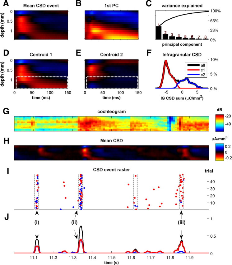
CSD events may fall into a small number of distinct classes. One of the main distinguishing features of event classes is the amount of infragranular activation. A, Average of all CSD events identified in the responses to the rock music stimulus recorded from one multi-electrode penetration. B, First PC of the distribution of CSD event shapes in this recording. The feature that explains the greatest part of the variance of the distribution of shapes is characterized by large currents in infragranular layers. C, Histogram of the variance explained by each of the first 10 PCs, averaged across penetrations. The cumulative proportion of the variance explained by the PCs is also shown. The first PC shown in B accounts for >30% of the variance in CSD event shapes and accounts for more than twice as much variance than any of the other PCs. D, E, When the CSD events in this electrode penetration are partitioned into two clusters by k-means clustering, the centroids of the CSD event clusters obtained have shapes as shown here. These differ prominently in their amount of infragranular activation (highlighted by the dashed white box) as might be expected from the PCA shown in B and C. F, Histogram of infragranular (IG) activation across CSD events in this penetration, as measured by integrating the CSD over the time intervals and infragranular depths delineated by the dashed white boxes in D and E. Black line gives the histogram for all CSD events, colors for each cluster, respectively. G, Cochleogram of the rock music stimulus. H, Trial-averaged CSD profile recorded during a 1 s segment of the rock music stimulus for the same penetration that yielded the data for A, B, and D–F. I, Raster of single-trial CSD events for the data in H. Events are colored red if they belong to the cluster shown in D, blue if they belong to the cluster shown in E. J, Probability of observing a CSD event in 20 ms windows at a particular trial. Black line for all events, red and blue for each cluster separately as in I. Across the whole dataset, the proportions of event types (red and blue dots), in time windows in which >10 events occurred, differed significantly from that expected by chance, and provided additional stimulus related information (see Results).

The first 10 PCs were usually enough to represent approximately three-quarters of the total variance. To reduce the dimensionality of the event shapes, we projected them onto their first 10 PCs and then performed k-means clustering on the space of the coefficients of the first 10 PCs. This typically segregated the data into two clusters: a cluster of CSD events with infragranular excitation and another one without (see Fig. 10D,E).

We quantified the extent of infragranular activation in each CSD event by integrating the infragranular CSD amplitudes over depths from 0.8 to 1.4 mm and from 5 to 150 ms after the onset of the CSD event. The distribution of infragranular CSD amplitudes within each electrode penetration was always strongly separated by the two clusters and was usually well fit by a mixture of two to six Gaussians. To account for skew in these distributions, we also fit a mixture of skew-normal distributions (Azzalini and Valle, 1996); for 19 of 24 penetrations, a mixture of two or more skew normals was required for a good fit. This strongly suggests that the CSD events are not associated with a single, homogeneous distribution of infragranular activations. For 4 of 24 of the penetrations, these distributions showed a significant bimodality (see Results; see Figs. 10F, 11).

Figure 11.

Distribution of infragranular activation during CSD events, for five example electrode penetrations. A, Centroids of the first cluster, with infragranular activation, shown for five electrode penetrations. B, Centroids of the second cluster, without infragranular activation. C, Distribution of the infragranular (IG) CSD sum of the detected events, as in Figure 10F. Black line gives the histogram for all CSD events, colors for each cluster, respectively. D, For each penetration, we used maximum likelihood methods to fit the empirical distribution of infragranular CSD sums (gray bars) with a mixture of Gaussian (MoG) model (colored lines, constituent Gaussians; black line, resulting MoG model). As the empirical distributions ranged from skewed unimodal distributions (e.g., top row) to bimodal and multimodal distributions (bottom 3 rows), so the number of Gaussians required for the best fit ranged between 2 and 6, with a mean of 3.4 across all penetrations. The empirical distributions were always better described by a mixture of Gaussians than by a single Gaussian. E, Because many of the empirical distributions had significant skew, we repeated the method in D by fitting a mixture of skew-normal (MoS) distributions (Azzalini and Valle, 1996). This typically reduced the size of the best mixture model. Although the empirical distributions were best fit by a single skew normal for 5 of 24 penetrations, the majority required a mixture of two or more. The mean number required was 2.6. This strongly suggests at a categorical nature to infragranular activation.

To establish whether the degree of infragranular activation was related to the degree of granular activation, we calculated the correlation coefficient between these values and those obtained by integrating CSD amplitudes over depths from 0.6 to 0.7 mm and from 5 to 60 ms after the onset of the CSD event.

Information in the amount of activation of the infragranular layers

To test the hypothesis that the event class is stimulus informative, we represented each single-trial CSD response as a ternary sequence. Each element represented a 20 ms time window and took the value 0 if there were no CSD events in the corresponding 20 ms window, 1 if there was a CSD event with weak or no infragranular activation (i.e., belonging to the first class), and 2 if there was a CSD event with strong infragranular activation (i.e., belonging to the second class). Next, we compared the amount of stimulus-related information carried in the set of ternary sequences with that carried by the set of sequences in which the time bins coded as 1 or 2 were randomly permuted. We used the same bias correction procedures detailed above to calculate stimulus-related information for the original and the permuted response sequences. We restricted this analysis to stimulus windows that elicited CSD events in at least 10 trials, to focus on those stimulus regions in which CSD events may have a role in stimulus coding.

Results

To understand how informative slow cortical fluctuations arise within the laminar circuitry of neocortex during complex sensory stimulation, we recorded LFPs and CSDs simultaneously at 16 depths, spaced at regular 100 μm intervals through the entire depth (from 0 to 1500 μm) of the A1 of four adult anesthetized rats, while presenting the acoustic stimuli described in Materials and Methods. We recorded from 24 electrode penetrations. The structure of our report is as follows. We first show that presenting simple stimuli produces large-amplitude events in the thalamic recipient layer. We then show that these events also encode complex stimuli and that these events are indeed the main cause of phase information. Finally, we consider how the activation associated with these events spreads through the cortical layers.

LFP and CSD responses to tonal stimulation

Before investigating responses to complex sounds, we first characterized the acoustic frequency tuning of each recording site by measuring responses to pure tones of varying frequency and intensity (Fig. 1A). Following Szymanski et al. (2009), we estimated the CF of each electrode penetration as the pure-tone frequency with the lowest intensity threshold for eliciting LFP responses. The trial-averaged LFP response to a 70 dB SPL tone at the CF is shown for an example penetration in Figure 1B. The presentation of the tone elicited an increase in the LFP magnitude at 20–40 ms after stimulus over a wide range of depths (between 400 and 1200 μm).

To identify the laminar origin of the sources generating the LFP signal, we subjected the data to CSD analysis (Mitzdorf, 1985; Petersen et al., 2006). The precise relationship between physiological currents in the cortical column and the observed LFP is complex and depends on details of the geometry and biophysics of the surrounding neuropil (Mitzdorf, 1985); nevertheless, current sinks seen in the CSD are usually interpreted as an estimate of the net depolarizing, excitatory currents entering the neurons at a particular depth and point in time. Current sources, meanwhile, are attributed to hyperpolarizing currents attributable to either inhibition or “return currents,” which occur, for example, when the excitatory charge that enters pyramidal cells in the middle layers leave through apical dendrites that project up to layer I.

The trial-averaged CSD for the same example penetration as in Figure 1, A and B, is shown in Figure 1C. In this example, the earliest sink arises at a depth of ∼1200 μm from the surface (approximately the bottom of layer V, top of layer VI) ∼10 ms after stimulus onset. This is followed almost immediately by a much stronger current sink at 400–500 μm (approximately the top of IV, deep layer III). These early sinks most likely reflect depolarization triggered by thalamic inputs. The observed CSD patterns are in agreement with previous accounts of the order of activation in the rodent primary auditory cortex, in which responses with very short latency are found not only in the chief thalamo-recipient layers in auditory cortex (lower layer III and layer IV; Smith and Populin, 2001) but also in the deepest cortical layers. This has been observed in rats (Kaur et al., 2005; Szymanski et al., 2009), mice (Shen et al., 1999), gerbils (Sugimoto et al., 1997), and guinea pigs (Wallace and Palmer, 2008). The neural activity triggered by the afferent input, near 500 μm (deep layer III and layer IV), then spreads upward to supragranular layers, as well as downward to infragranular layers. The short-latency sinks at depths of ∼500 μm (i.e., near layers III and IV) are accompanied by prominent return current sources in layer I (0–200 μm) (Szymanski et al., 2009).

CSD “events” during presentation of complex sounds

For each electrode penetration, we recorded responses to two different types of complex acoustic stimuli. These sounds exhibit rich real-world spectrotemporal dynamics and are effective at driving responses in auditory cortex. The first such dynamic stimulus was a 30-s-long segment of rock music, containing sounds from electric and percussion instruments along with a singing male human voice. The second stimulus was a 22-s-long synthetic dynamic-sine complex, with third-octave-spaced frequency components. The frequency and amplitudes of these components fluctuated randomly, with a 1/f-distributed power spectrum. This 1/f stimulus is also highly effective in driving cortical neurons (Garcia-Lazaro et al., 2006). Unlike the rock music, the 1/f stimulus lacked regular rhythms, percussive transient sounds, melodic structure, or other higher-order statistics that characterize a piece of music. Representative examples of single-trial CSD profiles during acoustic stimulation with rock music are shown in Figure 2B. We observed that these profiles undergo periods of relative inactivity (low amplitude), punctuated by discrete, large-amplitude “events” happening every few hundred milliseconds. The events closely resembled the CSD profiles recorded in response to an isolated pure tone at CF (compare with Fig. 1C). In particular, these events were characterized by a brief (∼50 ms), prominent dipole spanning the granular and supragranular layers (<700 μm).

Figure 2.

CSD events entrain to stimulus features. A, Cochleogram (spectrographic) representation of a 2 s segment of the rock music stimulus. B, CSD profiles recorded in one multi-electrode penetration in response to three individual presentations of the stimulus shown in A. The dashed yellow lines show CSD events detected by our algorithm. C, The black dots provide a raster display of CSD events detected during 50 stimulus repetitions. The blue line shows the observed CSD event rate as a function of time after the start of the music stimulus, and the red line shows the event rate predicted from a linear–nonlinear model, comprising the linear STRF of the CSD events shown in D. The prediction of the model captures 47% of the variance in the observed distribution of CSD events for this penetration. D, STRF of the CSD events recorded in response to the rock music stimulus. The observed best frequencies in this STRF (∼2–3 kHz) correlate well with those found in this penetration during stimulation with isolated pure tones. E, Static output nonlinearity for the penetration whose STRF is shown in D. The full linear–nonlinear prediction of the model is generated by first convolving the stimulus with the STRF and then passing the output of this (linear) function through a static nonlinear function. Here we fit a sigmoid function as the output nonlinearity. F, Autocorrelogram of CSD event times for the different stimulus conditions, averaged across multi-electrode penetrations. Note the ∼300 ms refractory period in all stimulus conditions. The autocorrelogram obtained with the rock music stimulus features regular peaks every 250 ms, marking an entrainment of the CSD events to the regular beat of the music. G, Power spectra of the LFP and CSD traces recorded at a depth of 0.5 mm, averaged across multi-electrode penetrations.

CSD events encode complex sound stimulation

To investigate quantitatively the role of these CSD events in stimulus processing, we developed an algorithm that automatically detected such CSD events within single-trial CSD profiles. The algorithm (fully detailed in Materials and Methods and schematized in Fig. 3) compared the CSD response in the supragranular layers (topmost eight channels; 0–700 μm) with a template derived from the average CSD response to pure tones at CF recorded at each recording site. Figure 2B shows three single-trial CSD responses to presentation of rock music, in which CSD events detected by our algorithm are marked by dashed lines. This figure suggests that there may be certain times within the rock music stimulus, such as at 1.18 s (i) and at 2.64 s (iv), when CSD events are likely to occur. Figure 2C shows the raster plot of CSD event times across all 50 available trials for this electrode penetration. This confirms that both the occurrence and the timing of CSD event times can be strongly dependent on the stimulus: both the probability that events occur and the trial-to-trial jitter in their timing varied as a function of time after the onset of the stimulus. In this example, CSD events occurred reliably and with precise timing (∼4 ms jitter) at 1.18 s (i) and at 2.64 s (iv), but a more variable event distribution is evident at 1.68 s (ii) and 2.41 s (iii), where jitter is ∼8 ms.

The stimulus dependence of CSD events may be at least partly explainable in terms of tuning to the spectrotemporal content of the stimulus. To show this, we computed the STRF of CSD events from responses to the rock stimulus, in a manner identical to that normally used for spike responses (Sahani and Linden, 2003). We correlated the time histogram of CSD events with a cochleogram representation of the stimulus (i.e., a spectral decomposition that mimics the cochlear encoding of the sound; see Patterson et al., 1987; Hohmann, 2002 and Materials and Methods for details). The CSD event STRFs were localized in frequency space, demonstrating that CSD events have a defined frequency tuning. Figure 2D shows the CSD event STRF for the electrode penetration also shown in Figure 2, B and C. The best frequencies of the STRFs correlated with the CFs obtained from pure-tone stimuli in the same penetration (r = 0.43; p < 0.05).

We then verified that the STRFs indeed captured the stimulus tuning of CSD events by using the STRFs in the context of a linear–nonlinear model (Chichilnisky, 2001; Simoncelli et al., 2004; Rabinowitz et al., 2011) to predict when CSD events would occur. The prediction was generated as follows. First, we convolved the STRF with the cochleogram representation of the sound to predict the CSD event distribution and passed the resulting linear prediction through a static output nonlinearity (Fig. 2E). This predicted CSD event rates that could then be compared against the observed CSD event distributions. The red and blue lines in Figure 2C illustrate predicted and observed CSD event rates, respectively. In this example, the STRF model captures 47% of the variance of the observed CSD events distribution. On average, over all penetrations, the STRF model explained 31% of the variance of the CSD event distribution. CSD events are therefore at least partially tuned to the spectral content of the stimulus. However, their stimulus dependency is only partly explained by the relatively simple STRF models used here.

CSD events occur also during spontaneous activity

CSD events were found not only in response to the rock music stimulus but also to the 1/f stimulus and even during periods of silence. Their rate of occurrence was similar across all these conditions, covering a range of ∼2–4 Hz (Fig. 3C). CSD events occurred at a slightly higher rate under rock music than in silence or in the presence of the 1/f stimulus (one-way ANOVA; p < 0.05). The autocorrelogram of CSD events (computed as an unbiased autocorrelation function as described by Orfanidis, 1988 and reported in Fig. 2F) illustrates that CSD events exhibited a refractory period in all stimulus conditions: consecutive events rarely occurred within intervals shorter than 300 ms. For the rock music stimulus only, events often occurred with a regular periodicity of 250 ms, marking an entrainment to the regular beat in that stimulus.

CSD events reset the CSD and LFP phase

Previous work (Luo and Poeppel, 2007; Kayser et al., 2009; Chandrasekaran et al., 2010) reported that complex sounds are encoded by the instantaneous phase of low-frequency (<15 Hz) LFPs and MEG signals recorded form auditory cortex, because the phase of these signals reliably aligns at specific times during complex auditory stimulation. It is natural to hypothesize that the discrete, large-amplitude CSD events that we reported above may be related to the phase encoding reported in previous studies.

To explore the relationship between CSD events and the phase of CSDs and LFPs, we considered two alternative approaches. We bandpassed the CSD and LFP signals in 15 different frequency bands, with center frequencies between 2 and 60 Hz. This narrowband analysis is useful for several reasons. First, it facilitates comparison with other previous studies (Lakatos et al., 2005, 2007, 2008, 2009; Lee et al., 2005; Montemurro et al., 2008; Kayser et al., 2009; Siegel et al., 2009) that have also used similarly bandpassed signals. Second, the band separation might reveal information in low-amplitude, high-frequency parts of the signal (e.g., in the gamma range) that might otherwise be obscured by large-amplitude, low-frequency events in the wideband signal or vice versa. A potential disadvantage of this approach is that bandpass filtering can introduce filter ringing artifacts. Such artifacts will be particularly marked if the chosen filters are narrow and sharp and if they are used on signals that contain sudden transients, such as the high-amplitude CSD events. To test that any results from the analysis of the narrowband-filtered signals presented here were not filtering artifacts, we therefore also performed analogous analyses on a wideband [2–60] Hz version of the CSD signal. The pass band of the wideband signal was sufficiently broad (almost 5 octaves) that any contamination of the ongoing phase of this signal by filter ringing would be minimal. Our observation that phase information is robust in the wideband signal is therefore a useful control. Conversely, the (Hilbert) phase of a wideband signal, although mathematically well defined, does not lend itself to an easy intuitive interpretation. To help the readers appreciate what the phase of the wideband signal represents, we draw attention, first, to the fact that the power in the wideband signal (and hence its instantaneous Hilbert phase) was dominated by low frequencies (Fig. 2G), and, second, that CSD events induce consistent and reproducible phase relationships across different frequency bands, as we illustrate in Figure 4.

Figure 4.

Single-trial CSD events and their relationship with the instantaneous phase. A, Example of a wideband (WB) LFP response in one multi-electrode penetration. B, CSD responses derived from the LFPs in A. C, D, The above responses, bandpass filtered with a [7–11] Hz pass band. E, F, LFP and CSD signals, respectively, at a depth of 500 μm below the pia. The top three traces show the LFP bandpassed in the [16–26] Hz band, the middle three traces in the [7–11] Hz range like in C, and the three bottom traces are wideband as in A. The traces are color coded as a function of their phases, as indicated in inset to F: [0, π/2), yellow; [π/2, π), green; [π, 3π/2), blue; [3π/2, 2π), red. G, H, Phases of the LFP and CSD as in E and F, but here responses to 10 repetitions of the stimulus are shown (as color code only) to illustrate the reproducibility of phase resets across trials and frequency bands.

Figure 4A–D shows single-trial LFP and CSD profiles from a sample penetration, both wideband and bandpassed at [7–11] Hz. Figure 4, E and F, shows the amplitudes and phases of these signals, in two narrowband and in the wideband condition, for three trials at a sample depth of 500 μm. It is readily apparent that the phases of both narrowband and wideband LFPs are reproducible and consistent across frequency bands only at the times when CSD events were reliably evoked, i.e., at ∼6.4 s (i), 6.65 s (ii), and 6.9 s (iii) poststimulus onset, and the phase values seen at those times, close to 3/2 π, are those one would expect if the CSD events are dominated by a brief, large-amplitude, negative-going transient. Figure 4, G and H, confirms that this phase consistency across frequency bands, which is seen near CSD event times only, is reproducible across many trials and hence carries stimulus-related information.

The relationship between CSD events and reproducible signal phase is further illustrated in Figure 5, which uses data from the same example penetration in response to rock music as in Figure 4 at 500 μm depth. Figure 5A shows that, before the onset of CSD events, the phases of [7–11] Hz filtered LFPs at 500 μm depth could take on any value with almost equal probability. However, the onset of CSD events coincided with a dramatic sharpening of the phase distribution. Then, from ∼100 ms after the CSD event, the phase distribution broadened out as time after the event increased. Similar observations were made at different depths in the 500–900 μm range and in other low frequency bands and in the wideband signal (results not shown). Thus, CSD events coincide with a phase resetting of the LFP.

Figure 5.

CSD events correspond to a resetting of the LFP phase. A, The distribution of LFP phases in the [7–11] Hz band, at a depth of 500 μm, as a function of time relative to the onset of CSD events. The LFP phase distribution is broad before the onset of CSD events (t < 0) but then sharpens dramatically as the CSD event unfolds. B, Periods of high LFP phase coherence are initiated during the same stimulus episodes as when CSD events typically occur. Top, Three seconds of the rock music stimulus. Middle, LFP phase in the [7–11] Hz band at a depth of 500 μm, over 25 repeats. Colors as in Figure 4E–H. Black circles denote the times of detected CSD events in the respective trials. Bottom, The coherence of LFP phases (shown in black for the [7–11] Hz band and gray for the wideband) relative to a probability histogram of the CSD events (shown in red). WB, Wideband. C, Black line, CSD-event-triggered phase coherence of the LFP phase in the [7–11] Hz band and at a depth of 500 μm. Gray line, Event-triggered coherence of the wideband LFP signal. The phase coherence values are temporally aligned to the times of CSD events (t = 0) and averaged across all events. The onset of the CSD event coincides with a rapid rise and subsequent decay in phase alignment, which takes ∼100–200 ms. CSD events therefore mark a transition from periods in which LFP phase is unreliable across trials to a period in which phase is reliably stimulus locked. All data in this figure are taken from a single example recording session (same as in Fig. 4) in response to the rock music stimulus.

Because CSD events occur at reliable points during the stimulus and because they align LFP phase across a wide range of frequencies, it seems highly likely that CSD events are the main cause of “phase resets” in our preparation. When considering any one stimulus episode, the relationship between CSD events and phase reliability across trials is striking. Figure 5B shows how, across many repetitions of a stimulus (top panel), periods of high LFP phase coherence (shown for the [7–11] Hz band and the wideband) were initiated at the same time as when CSD events typically occurred. Conversely, immediately after any CSD event occurred during a single trial of a stimulus presentation, there was a high probability that LFP phase was highly coherent across trials for those stimulus episodes. This phase coherence (both the wideband and the narrowband LFP; Fig. 5C) decayed over a period of 100–200 ms after the time of the event and was relatively low immediately before the next event.

Together, these results suggest that the informativeness of LFP and CSD phases about complex stimuli seen by both us and others (Kayser et al., 2009; Chandrasekaran et al., 2010) arises from phase alignments occurring at specific, discrete time points during stimulus presentation rather than from an internal clock providing a reliable phase signal at all times. The fact that the wideband analysis gives very similar results to those seen in the bandpass analysis not only confirms that filter ringing artifacts do not significantly affect our results, it also underlines the broadband, “impulse-like” nature of the phase-resetting events.

Information content of the LFP and CSD in response to ongoing, complex stimulation

It has been documented previously that LFP, MEG, or EEG phase encodes information about complex stimuli (Luo and Poeppel, 2007; Kayser et al., 2009; Schyns et al., 2011). The evidence we present above suggests that CSD events are a key determinant of this encoding. To test this hypothesis further, we first considered how phase information in the LFP and CSD is distributed across layers. Following Montemurro et al. (2008) and Kayser et al. (2009), we computed the mutual information carried by CSD/LFP phases about which part of the dynamic stimulus was being presented. This formalism (schematized in Fig. 6) makes no assumptions about which sound features in the stimulus are encoded by the neural signals; rather, it measures how much information about all possible stimulus attributes can be gained from observing a single trial of the LFP/CSD phase (de Ruyter van Steveninck et al., 1997). As above, we performed these analyses in 15 frequency bands as well as on the wideband signals.

Figure 6.

Illustration of the computation of mutual information between CSD/LFP phase and the stimulus. This figure sketches how we computed the information carried by the CSD/LFP phase about which section of the dynamic stimulus was being presented. We first binned the signal phase into quadrants at each time point during stimulus presentation. A shows an example of these sequences across 25 repeated presentations of 1.2 s of rock music, with phase quadrants color coded as in Figure 4F. We next determined the distribution of phase quadrants across trials, for each time point. These distributions are exemplified in B and C for two example time points. We used Equation 1 in Materials and Methods to calculate the information, using the distribution of phases at each time point, and the distribution of phase across all time points (reported in D). Equation 1 quantifies how dissimilar the phase probabilities at each time are from each other and from the distribution of phases across all time points and trials.

For the narrowband phase, the average information carried by signal phase about either rock music or 1/f sounds over all electrode penetrations is reported in Figure 7, as a function of penetration depth and frequency band. Across all recording depths, the information carried by both CSD and LFP phase was greatest in the low-frequency bands (CFs of ∼4–16 Hz). The main difference between LFP and CSD phase information was in their respective distribution across layers. LFP phase information was broadly spread across depths, with a maximum at depths between 400 and 800 μm (Fig. 7A). In comparison, the CSD phase information was more localized and had clear, distinct maxima at two different depths: one at the surface of the cortex (layer I), the second at ∼600 μm (granular input layers; Fig. 7B). These are the same depths as the prominent dipole in CSD events (Figs. 1C, 3A). This provides support to the hypothesis that these large, relatively stereotyped events play a key role in setting up informative CSD and LFP phases.

Figure 7.

Depth–frequency profiles of the information between the phase of the LFP (A) or CSD (B) and the stimulus. Data are averaged across penetrations; information values are shown according to the color scale on the right. The top row shows information depth profiles obtained with the rock music stimuli, and the bottom row shows the values obtained with the 1/f stimuli. CSD information (B) was localized to the surface of the cortex (∼0 μm) and the granular input layers (∼600 μm), whereas the LFP information (A) was broadly distributed. These sources of stimulus information were highly redundant (Fig. 8). The colored column to the right of each plot displays the phase information in the wideband (WB) signal.

The information in the high-frequency (gamma) range (>40 Hz) was small at all depths in both CSD and LFPs. This finding is consistent with the view that the reliable phases observed in LFPs do not originate from an internally generated rhythm that is of high frequency, low amplitude, and high reliability (Fries et al., 2007).

The wideband signal also yielded phase information with a very similar spatial profile to that of the narrow bands (colored column to the right of each plot in Fig. 7). This argues for a common cause of the phase information in each frequency band.

Redundancy of phase information across cortical layers

Although the CSD phase is most informative about the stimulus at two depths—near the surface and in the granular layers—these two signals may share the same or have different information about the sound stimuli. To distinguish between these possibilities, we computed the amount of information redundancy between the CSD phase at these two depths. We found that the CSD phase information at these two depths was highly redundant (Fig. 8B). For example, in the [10–16] Hz frequency band during presentation of the rock music stimulus, the redundancy in the CSD phase information at depths 0 and 0.5 mm was 0.09 bits, whereas the information in the CSD phase at 0.5 mm was 0.23 bits. Here, the redundancy was 39% of the maximum possible (see Eq. 5). This suggests that the fluctuations in the CSD observed at these depths express a single common underlying neural cause. Moreover, we found that the LFP phase information shared this same common origin. In the layers in which LFP phase information was maximal, it was highly redundant with both the thalamo-recipient and superficial layers of the CSD (Fig. 8C). The redundancy between the LFP at depth 0.5 mm and the CSD at the same depth is 0.11 bits, whereas the information in the CSD and the LFP at this depth was 0.23 and 0.19 bits, respectively. This in turn implies that the redundancy between CSDs and LFPs at 0.5 mm depth was 55% of the possible amount of redundancy.

Figure 8.

Information redundancy in LFPs and CSDs. A, Redundancy between the information in the LFP phases at different depths for the rock music stimulus (top) and 1/f stimulus (bottom), for the [7–11] Hz band. Redundancy values are computed through Equation 3 and are expressed in bits. B, Redundancy between the information in the CSD phases at different depths for the [7–11] Hz band. C, Redundancy between the information in the LFP phase and that in the CSD phase recorded at different depths, for the [7–11 Hz] band. As for A and B, for the rock music (top) and 1/f stimuli (bottom) separately.

Together with the close correspondence between the laminar pattern of CSD information and the main current dipole that spans the supragranular layers in the pure-tone-evoked CSD profiles (Fig. 1C), these results strongly suggest that the common origin of most, if not all, of the stimulus-related information in LFP and CSD phases throughout rat primary auditory cortex is the thalamic input to granular layers. This input manifests as strong, depolarizing current sinks at 600 μm, which are accompanied by return currents flowing through apical dendrites of deep layer III/layer IV pyramidal cells, to exit in layer I.

CSD events mark episodes of high-stimulus-related information in the LFP phase

The results above suggest that the informativeness of LFP phase is the result of reliable CSD events, and, as a consequence, information about the stimulus in the phase should be temporally localized around the times of CSD events. This is because the events mark a transition from a period in which LFP phase is unreliable across trials—and hence can carry little information about the stimulus—to a period of high LFP phase coherence in which phase can be informative.

We tested this idea quantitatively by scrambling the LFP phase in short windows of 150 ms duration and measuring the effect on information. The time windows were positioned either so as to start immediately after the onset of each CSD event, or to precede it, or else to occur at random times unrelated to the timing of CSD events. The effect of this targeted phase scrambling is illustrated in Figure 9. Scrambling the LFP phase immediately after the onset of the events indeed destroyed most of the stimulus-related information and did so at all depths and in all LFP frequency bands. In comparison, scrambling 150 ms of the LFP phase around an equal number of randomly chosen “pseudo-event” times also reduced the amount of stimulus-related information available in the LFP phase but considerably less so than the targeted scrambles. Finally, scrambling the period immediately before the onset of CSD events was least detrimental to phase information. For example, for the rock stimulus and for phase in the [7–11] Hz frequency band and at 0.5 mm depth, scrambling after the onset of CSD events destroyed an average of 78% of the phase information, scrambling around random times destroyed 61%, and scrambling immediately before CSD events destroyed 55%.

Figure 9.

The bulk of LFP phase information coincides with CSD events. A, LFPs recorded in one electrode penetration in response to a 1 s segment of the rock music stimulus and averaged across 25 trials. B, LFP phase in the [7–11] Hz band in the same penetration as that shown in A, at a depth of 500 μm, across 25 trials. Color convention is the same as Figure 4F; the times of CSD events are shown as black circles. In the four rows, LFP phase has either been left unchanged (top row) or scrambled over a window of 150 ms. These windows either began at the same time as CSD events (second row), began at random times (third row), or ended at the same time that CSD events began (bottom row). C, Depth–frequency profiles of stimulus-related information in the LFP phase for the rock music stimulus, plotted as in Figure 7A. The purple circle indicates the [7–11] Hz band at a depth of 500 μm, as illustrated in B. Rows show the effect of scrambling the phase as in B. The most detrimental time to scramble was immediately after CSD event onset: this destroyed 76% of the information for the example band and depth compared with 60% for scrambling at random times and 55% for scrambling immediately before CSD event onset. D, Same as C but for the 1/f stimulus.

As with the narrowband signals, information in the phase of the wideband signal was also localized around the times of CSD events. When considering the phase of the LFP in this signal at 0.5 mm depth in response to the rock stimulus, scrambling after the onset of CSD events destroyed an average of 82%, scrambling around random times destroyed 60%, and scrambling immediately before CSD events destroyed 48%. Applying the same procedure to CSD rather than LFP phases yielded very similar results (data not shown).

CSD event classes

Our CSD event detection algorithm operates by recognizing a stereotypical CSD activation pattern in the supragranular layers. It exploits the fact that CSD events tended to exhibit consistent patterns of supragranular activation (Fig. 2B). However, the detection algorithm did not constrain the pattern of infragranular activation. Indeed, CSD events may fall into a number of distinct classes, which differ in aspects such as the extent and nature of infragranular activation. We investigated the morphological diversity of CSD events using PCA. Figure 10, A and B, compares the average CSD event morphology with that of the first PC of the event shape distribution for one multi-electrode penetration. This first PC features a pronounced infragranular current sink, which is accompanied by return current sources in the supragranular layers. Across all electrode penetrations, the first PCs invariably showed such infragranular features and explained on average >30% of the variance in the shape of CSD events (Fig. 10C).

Similarly, when the CSD events were assigned to one of two classes using an unsupervised k-means clustering algorithm (for details, see Materials and Methods), the resultant clusters always separated those CSD events featuring strongly activated infragranular layers from those which did not. The centroids of the clusters obtained when clustering the CSD events whose mean was shown in Figure 10A are illustrated in Figure 10, D and E. The differences in the amount of infragranular activation (areas bounded by white dashed lines) are readily apparent.

Because the amplitude of infragranular CSD sinks is thought to capture the “output” layers of cortex, which project heavily to subcortical targets (Douglas and Martin, 2004; Thomson and Lamy, 2007), it is interesting to consider how activation in infragranular layers during a CSD event correlates with activation in the supragranular and granular layers. The average correlation coefficient between these measures across penetrations (see Materials and Methods) was modest (r² = 0.14 ± 0.03). Insofar as the ratio of granular–supragranular to infragranular activation is representative of the computation within a cortical column, this computation therefore appears to involve more than a simple scaling or thresholding of the input activation.

An interesting but difficult question to answer is whether these infragranular outcomes can be adequately described in terms of a small number of discrete and distinct activation states. This number may be as small as two, corresponding to “on” and “off” states of infragranular circuits. The partitioning of events illustrated in Figure 10, D and E, cannot answer this question, because k-means clustering simply seeks a sensible division of the data into the number of clusters requested (two in the case shown here) and does not provide a good tool for determining the “true” number of natural partitions or clusters within the data. In the case shown in Figure 10, D and E, one can make a strong case for the fact that there are indeed two distinct classes, because the distribution of infragranular CSD amplitudes, integrated over the time intervals and depths shown by the white dashed lines, forms a bimodal distribution, as shown in Figure 10F. However, in only 4 of 24 electrode penetrations examined did the distributions of infragranular CSD amplitudes exhibit statistically significant bimodality (Hartigan's dip test, p < 0.05). Nevertheless, 19 of 24 of these distributions were better described by a mixture of two or more unimodal distributions (normal or skew normal) than by a single such distribution (Fig. 11), arguing that the distribution of CSD events are not associated with a homogeneous continuum of infragranular activation. Although this will need additional study in the future with larger datasets and more sensitive methods, our results do indicate that a categorization of CSD events—into those that trigger large infragranular activity and those that do not—captures an important aspect of the diversity of CSD events, even if the true underlying distribution may often be more complex.

Crucially, we found that the amount of infragranular activation accompanying a CSD event is, to some extent, stimulus dependent. This was evident from the distribution of the two CSD event classes over time within a penetration, as illustrated in Figure 10, I and J. In this example, although at the stimulus episodes at 11.12 s (i) and 11.34 s (ii) either CSD event type was about equally likely, the stimulus episode at 11.85 s (iii) was approximately four times more likely to trigger CSD events with infragranular activation than CSD events without. To assess these data statistically, we calculated the proportion of “class I” (strong infragranular activation) events in all stimulus episodes that elicited CSD events in at least 10 repeat presentations. Indeed, the distribution of CSD event classes was significantly different from that expected by chance (binomial test; p < 0.05)—and therefore significantly dependent on stimulus history—in 75% of our datasets recorded with the rock music stimulus and for 82% of our datasets recorded with the 1/f stimulus.

Finally, we estimated how much additional information about the stimulus is carried by the activation state of the infragranular layers. This was done by computing the mutual information between the stimulus and the response, in which the latter was allowed to take one of three values: CSD event with strong infragranular activation, CSD event without such infragranular activation, or absence of CSD event altogether. We then scrambled any information about the stimulus that may have been encoded in the infragranular activation by randomly reassigning each CSD event to one of the two subclasses. During rock music stimulation, infragranular activation carried a median 22% more information about the stimulus than the random reassignments for the 20 of 23 penetrations in which this difference was significant (t test, p < 0.05). For the 1/f stimulus, this figure was 36%, for 9 of 11 penetrations. This analysis reveals that CSD events reflect the outcome of a stimulus-dependent calculation.

However, although the type of CSD event observed showed significant dependence on stimulus history, it is important to note that this effect was not very large. During repeat presentations of the same stimulus, many stimulus episodes were marked by mixtures of class I and class II events, as is readily apparent in the example shown in Figure 10I. We also investigated whether the apparent stimulus sensitivity of CSD event types could be captured by linear–nonlinear STRF models. However, we observed no statistically significant differences (data not shown) between such models fitted to class I or class II events, respectively, except for simple scale factors that arise from differences in event rates (class I events being generally more common than class II). Thus, although there is a significant interdependence between stimulus history and the type of the evoked CSD event, the nature of this dependence is not easily captured by standard linear–nonlinear receptive field models.

Discussion

Previous studies reported that low-frequency LFPs entrain to the sensory environment, and hence their phase becomes informative about sensory stimuli. We sought to trace the origin of informative LFP phase, by investigating the dynamics of CSDs during naturalistic stimulation. We found that the CSD traces were dominated by events with a stereotyped pattern of activity. The events were defined by a strong granular layer activation, characterized by brief (∼50 ms), large-amplitude current sinks in thalamo-recipient layers and current sources in superficial layers. This suggests that they reflect mostly bursts of thalamocortical activation, although it is conceivable that they may also reflect some corticocortical activation (Happel et al., 2010). Although such CSD events could occur spontaneously, in the presence of stimulation, they were nevertheless stimulus tuned. Importantly, CSD events coincided with a phase resetting of the LFP. Indeed, scrambling LFP phase specifically in small time windows after the onset of CSD events destroyed disproportionately large amounts of the stimulus-related information in the phase of low-frequency (<20 Hz) LFP (Fig. 9). Thus CSD-event-induced phase resetting appears to be a major factor in establishing stimulus-related information in the LFP.

CSD events produce reliable, informative phases in the LFP

The ability of low-frequency LFPs to follow the dynamics of complex stimuli is thought to be a key functional link between the temporal structure of sensory information and the fluctuating excitability of the neuronal ensembles involved in the processing of this information (Lakatos et al., 2009). The synchronization of the phase of LFPs with natural stimuli has been observed in both visual and auditory cortex and in both anesthetized and awake animals (Montemurro et al., 2008; Kayser et al., 2009), and it can in principle be generated in at least two ways: (1) they may reflect entrainment of an existing oscillation that is internally generated by the cortical circuitry, or (2) they arise from fluctuating input to the cortical network (Mazzoni et al., 2008). Our findings favor the second scenario, in that they suggest that volleys of strong lemniscal thalamic activation delivered to the granular layers of cortex—which we have described here as CSD events—are likely to be a major cause in generating this phase synchronization. These results therefore complement those of Lakatos and Schroeder (Lakatos et al., 2007, 2009), who have suggested that cross-modal phase alignments in auditory cortex are mediated by nonspecific, modulatory thalamic afferents, which project widely to superficial cortical layers of sensory cortex. Our study, in contrast, analyzed the laminar origin of phase information purely during within-modality stimulation. In our preparation, phase alignment appears to be the result of transient, large-amplitude events and can therefore be described, in the terminology of Lakatos et al. (2007, 2009) and that of Makeig et al. (2002) as being of the “evoked” or “driving” type.

Several recent studies have proposed that the phase of slow rhythms in non-invasive, EEG and MEG recordings in humans also carries significant information about complex naturalistic stimuli (Luo and Poeppel, 2007; Schyns et al., 2011), in the same manner as observed with invasive, intracranial LFP recordings in animals. As with LFP, the informativeness of phase signals from coarser measures of neural activity must depend, in turn, on some process of phase alignment. We speculate that this at least partly originates from transient, large-amplitude events of the type described in our study, reflecting fast activation of the thalamo-recipient layers of the cortex. This of course does not exclude the possibility that phase consistency during sensory processing may be controlled by several distinct mechanisms, including a combination of driving and modulatory phase alignments.

Are phase-resetting CSD events a manifestation of “bumps” or transitions into up states?

CSD events, as short bursts of excitation in the granular layers, are reminiscent of membrane potential “bumps” reported previously in rat auditory cortex (DeWeese and Zador, 2006): quiescent periods are punctuated by brief intermittent, highly synchronous and high-amplitude volleys. Intracellularly recorded bumps often co-occur with increases in LFP amplitude (Deweese and Zador, 2004). The largest such bumps are thought to stem from several hundred synchronized postsynaptic potentials, indicating that bouts of highly concerted firing among input neurons may be an integral part of the operation of auditory cortex. It thus seems conceivable that the CSD events we describe here are extracellular correlates of these intracellularly observed bumps.

We also observed that CSD events occur spontaneously at rates of a few hertz in the absence of stimulation. They may therefore be related to the stereotyped bursts of spiking activity observed by Luczak et al. (2009) in simultaneous recordings of large populations of isolated cortical neurons. The authors attribute such bursts as transitions into up states. Like the CSD events observed here, transitions into these excitable states can occur spontaneously or may be triggered by either thalamic inputs delivered electrically (MacLean et al., 2005) or sensory input (Petersen et al., 2003).

Functional implications of encoding stimulus-related information in LFP and CSD phase

Previous studies of stimulus encoding in the phase of LFPs (Montemurro et al., 2008; Kayser et al., 2009) have demonstrated that phase carries large amounts of information about which part of a complex dynamic stimulus was being presented but did not identify the specific aspects of the stimulus history that are explicitly represented in a neural signal. Here we found that some stimulus episodes reliably elicit strong depolarization in the thalamic recipient layers, which resets the LFP phase to a coherent, informative state and account for a large part of the stimulus-related information in LFP phases. One possibility is that LFP phase encodes the time elapsed since the last stimulus eliciting strong net depolarizing thalamic inputs to the local cortical region. The encoding of such times may be important for analyzing the temporal structure of sensory scenes and could provide a useful internal temporal reference frame linking spike times to salient aspects of stimulation history. This timeframe would enable phase-of-firing codes (Montemurro et al., 2008; Kayser et al., 2009) to enhance the information carried by the current firing rate by putting it in the context of recent stimulus dynamics. It is tempting to speculate that the robustness to background acoustic noise of phase-of-firing codes reported by Kayser et al. (2009) originates from the reliable temporal reference frame that is set up and maintained by CSD events.

Phase-resetting CSD events are accompanied by different types of infragranular activation patterns

Finally, we have shown that CSD events differ in their morphology. Although they begin with an initial trigger in the granular layers, this propagates—to a greater or lesser extent—into the supragranular and infragranular layers. These observations are consistent with current models of the feedforward component of information processing within cortex (Thomson and Lamy, 2007), which envisage a predominant flow of sensory signals into the granular layer, from there into layers II/III, and then down to layers V and VI. Therefore, these events may be taken as useful templates to characterize the dynamics of the feedforward propagation of sensory information during complex stimulation.

In this context, it is of considerable interest that the pattern of neural activity is not uniform across CSD events. The most notable variation is the extent to which infragranular output layers of the cortical column are activated. The distributions of infragranular activations across events were often either bimodal or best described as a mixture of a small number of unimodal distributions. These results raise the intriguing possibility that the response of the infragranular layers to the triggering of a CSD event in the supragranular layers may be in some sense quantal, i.e., the amount of infragranular activation may vary in a modest number of somewhat discrete steps.

Tantalizingly, the extent to which infragranular regions were activated was stimulus dependent. Insofar as the distribution of infragranular activations is indicative of a quantized or discrete underlying process, it may reflect a categorical evaluation of stimulus episodes. As the CSD event unfolds, the local circuit determines whether to pass on stimulus information through the output layers. This burst-like mode of operation of auditory cortical columns engaged in processing continuous complex sounds suggested by our data would imply that cortical columns alternate between states of high information transfer marked by CSD events that are interspersed by periods of relative quiescence and low information transfer. Future experiments designed to record and analyze single-unit data and CSD profiles simultaneously and in parallel should make it possible to test this prediction directly.

All in all, our findings lead us to conclude that event-based analysis of cortical CSD patterns that we have developed here may evolve into a powerful tool for observing the outcomes of computations of cortical columns in vivo. They provide a spatially and temporally detailed description of how complex stimuli are processed in the brain, which complements and exceeds that which can be gleaned from the phase and power of an individual frequency band or recording channel.

References

- Ahrens MB, Linden JF, Sahani M. Nonlinearities and contextual influences in auditory cortical responses modeled with multilinear spectrotemporal methods. J Neurosci. 2008;28:1929–1942. doi: 10.1523/JNEUROSCI.3377-07.2008. [DOI] [PMC free article] [PubMed] [Google Scholar]
- Averbeck BB, Latham PE, Pouget A. Neural correlations, population coding and computation. Nat Rev Neurosci. 2006;7:358–366. doi: 10.1038/nrn1888. [DOI] [PubMed] [Google Scholar]
- Azouz R, Gray CM. Cellular mechanisms contributing to response variability of cortical neurons in vivo. J Neurosci. 1999;19:2209–2223. doi: 10.1523/JNEUROSCI.19-06-02209.1999. [DOI] [PMC free article] [PubMed] [Google Scholar]
- Azzalini A, Valle AD. The multivariate skew-normal distribution. Biometrika. 1996;83:715–726. [Google Scholar]
- Chandrasekaran C, Turesson HK, Brown CH, Ghazanfar AA. The influence of natural scene dynamics on auditory cortical activity. J Neurosci. 2010;30:13919–13931. doi: 10.1523/JNEUROSCI.3174-10.2010. [DOI] [PMC free article] [PubMed] [Google Scholar]
- Chichilnisky EJ. A simple white noise analysis of neuronal light responses. Network. 2001;12:199–213. [PubMed] [Google Scholar]
- David SV, Mesgarani N, Shamma SA. Estimating sparse spectro-temporal receptive fields with natural stimuli. Network. 2007;18:191–212. doi: 10.1080/09548980701609235. [DOI] [PubMed] [Google Scholar]
- de Ruyter van Steveninck RR, Lewen GD, Strong SP, Koberle R, Bialek W. Reproducibility and variability in neural spike trains. Science. 1997;275:1805–1808. doi: 10.1126/science.275.5307.1805. [DOI] [PubMed] [Google Scholar]
- Deweese MR, Zador AM. Shared and private variability in the auditory cortex. J Neurophysiol. 2004;92:1840–1855. doi: 10.1152/jn.00197.2004. [DOI] [PubMed] [Google Scholar]
- DeWeese MR, Zador AM. Non-Gaussian membrane potential dynamics imply sparse, synchronous activity in auditory cortex. J Neurosci. 2006;26:12206–12218. doi: 10.1523/JNEUROSCI.2813-06.2006. [DOI] [PMC free article] [PubMed] [Google Scholar]
- Douglas RJ, Martin KA. Neuronal circuits of the neocortex. Annu Rev Neurosci. 2004;27:419–451. doi: 10.1146/annurev.neuro.27.070203.144152. [DOI] [PubMed] [Google Scholar]
- Fiser J, Chiu C, Weliky M. Small modulation of ongoing cortical dynamics by sensory input during natural vision. Nature. 2004;431:573–578. doi: 10.1038/nature02907. [DOI] [PubMed] [Google Scholar]
- Fries P, Nikolić D, Singer W. The gamma cycle. Trends Neurosci. 2007;30:309–316. doi: 10.1016/j.tins.2007.05.005. [DOI] [PubMed] [Google Scholar]
- Garcia-Lazaro JA, Ahmed B, Schnupp JW. Tuning to natural stimulus dynamics in primary auditory cortex. Curr Biol. 2006;16:264–271. doi: 10.1016/j.cub.2005.12.013. [DOI] [PubMed] [Google Scholar]
- Gawne TJ, Richmond BJ. How independent are the messages carried by adjacent inferior temporal cortical neurons? J Neurosci. 1993;13:2758–2771. doi: 10.1523/JNEUROSCI.13-07-02758.1993. [DOI] [PMC free article] [PubMed] [Google Scholar]
- Happel MF, Jeschke M, Ohl FW. Spectral integration in primary auditory cortex attributable to temporally precise convergence of thalamocortical and intracortical input. J Neurosci. 2010;30:11114–11127. doi: 10.1523/JNEUROSCI.0689-10.2010. [DOI] [PMC free article] [PubMed] [Google Scholar]
- Hatsopoulos NG, Ojakangas CL, Paninski L, Donoghue JP. Information about movement direction obtained from synchronous activity of motor cortical neurons. Proc Natl Acad Sci USA. 1998;95:15706–15711. doi: 10.1073/pnas.95.26.15706. [DOI] [PMC free article] [PubMed] [Google Scholar]
- Hohmann V. Frequency analysis and synthesis using a Gammatone filterbank. Acta Acust Acust. 2002;88:433–442. [Google Scholar]
- Kaur S, Rose HJ, Lazar R, Liang K, Metherate R. Spectral integration in primary auditory cortex: laminar processing of afferent input, in vivo and in vitro. Neuroscience. 2005;134:1033–1045. doi: 10.1016/j.neuroscience.2005.04.052. [DOI] [PubMed] [Google Scholar]
- Kayser C, Montemurro MA, Logothetis NK, Panzeri S. Spike-phase coding boosts and stabilizes information carried by spatial and temporal spike patterns. Neuron. 2009;61:597–608. doi: 10.1016/j.neuron.2009.01.008. [DOI] [PubMed] [Google Scholar]
- Koepsell K, Wang X, Hirsch JA, Sommer FT. Exploring the function of neural oscillations in early sensory systems. Front Neurosci. 2010;4:53. doi: 10.3389/neuro.01.010.2010. [DOI] [PMC free article] [PubMed] [Google Scholar]
- Lakatos P, Shah AS, Knuth KH, Ulbert I, Karmos G, Schroeder CE. An oscillatory hierarchy controlling neuronal excitability and stimulus processing in the auditory cortex. J Neurophysiol. 2005;94:1904–1911. doi: 10.1152/jn.00263.2005. [DOI] [PubMed] [Google Scholar]
- Lakatos P, Chen CM, O'Connell MN, Mills A, Schroeder CE. Neuronal oscillations and multisensory interaction in primary auditory cortex. Neuron. 2007;53:279–292. doi: 10.1016/j.neuron.2006.12.011. [DOI] [PMC free article] [PubMed] [Google Scholar]
- Lakatos P, Karmos G, Mehta AD, Ulbert I, Schroeder CE. Entrainment of neuronal oscillations as a mechanism of attentional selection. Science. 2008;320:110–113. doi: 10.1126/science.1154735. [DOI] [PubMed] [Google Scholar]
- Lakatos P, O'Connell MN, Barczak A, Mills A, Javitt DC, Schroeder CE. The leading sense: supramodal control of neurophysiological context by attention. Neuron. 2009;64:419–430. doi: 10.1016/j.neuron.2009.10.014. [DOI] [PMC free article] [PubMed] [Google Scholar]
- Latham PE, Lengyel M. Phase coding: spikes get a boost from local fields. Curr Biol. 2008;18:R349–R351. doi: 10.1016/j.cub.2008.02.062. [DOI] [PubMed] [Google Scholar]
- Lee H, Simpson GV, Logothetis NK, Rainer G. Phase locking of single neuron activity to theta oscillations during working memory in monkey extrastriate visual cortex. Neuron. 2005;45:147–156. doi: 10.1016/j.neuron.2004.12.025. [DOI] [PubMed] [Google Scholar]
- Luczak A, Barthó P, Harris KD. Spontaneous events outline the realm of possible sensory responses in neocortical populations. Neuron. 2009;62:413–425. doi: 10.1016/j.neuron.2009.03.014. [DOI] [PMC free article] [PubMed] [Google Scholar]
- Luo H, Poeppel D. Phase patterns of neuronal responses reliably discriminate speech in human auditory cortex. Neuron. 2007;54:1001–1010. doi: 10.1016/j.neuron.2007.06.004. [DOI] [PMC free article] [PubMed] [Google Scholar]
- MacLean JN, Watson BO, Aaron GB, Yuste R. Internal dynamics determine the cortical response to thalamic stimulation. Neuron. 2005;48:811–823. doi: 10.1016/j.neuron.2005.09.035. [DOI] [PubMed] [Google Scholar]
- Makeig S, Westerfield M, Jung TP, Enghoff S, Townsend J, Courchesne E, Sejnowski TJ. Dynamic brain sources of visual evoked responses. Science. 2002;295:690–694. doi: 10.1126/science.1066168. [DOI] [PubMed] [Google Scholar]
- Mazzoni A, Panzeri S, Logothetis NK, Brunel N. Encoding of naturalistic stimuli by local field potential spectra in networks of excitatory and inhibitory neurons. PLoS Comput Biol. 2008;4:e1000239. doi: 10.1371/journal.pcbi.1000239. [DOI] [PMC free article] [PubMed] [Google Scholar]
- Mitzdorf U. Current source-density method and application in cat cerebral cortex: investigation of evoked potentials and EEG phenomena. Physiol Rev. 1985;65:37–100. doi: 10.1152/physrev.1985.65.1.37. [DOI] [PubMed] [Google Scholar]
- Montemurro MA, Senatore R, Panzeri S. Tight data-robust bounds to mutual information combining shuffling and model selection techniques. Neural Comput. 2007;19:2913–2957. doi: 10.1162/neco.2007.19.11.2913. [DOI] [PubMed] [Google Scholar]
- Montemurro MA, Rasch MJ, Murayama Y, Logothetis NK, Panzeri S. Phase-of-firing coding of natural visual stimuli in primary visual cortex. Curr Biol. 2008;18:375–380. doi: 10.1016/j.cub.2008.02.023. [DOI] [PubMed] [Google Scholar]
- Nelken I, Rotman Y, Bar Yosef O. Responses of auditory-cortex neurons to structural features of natural sounds. Nature. 1999;397:154–157. doi: 10.1038/16456. [DOI] [PubMed] [Google Scholar]
- Okun M, Naim A, Lampl I. The subthreshold relation between cortical local field potential and neuronal firing unveiled by intracellular recordings in awake rats. J Neurosci. 2010;30:4440–4448. doi: 10.1523/JNEUROSCI.5062-09.2010. [DOI] [PMC free article] [PubMed] [Google Scholar]
- Orfanidis SJ. Optimum signal processing: an introduction. Ed 2. New York: Macmillan; 1988. [Google Scholar]
- Panzeri S, Treves A. Analytical estimates of limited sampling biases in different information measures. Network. 1996;7:87–107. doi: 10.1080/0954898X.1996.11978656. [DOI] [PubMed] [Google Scholar]
- Panzeri S, Senatore R, Montemurro MA, Petersen RS. Correcting for the sampling bias problem in spike train information measures. J Neurophysiol. 2007;98:1064–1072. doi: 10.1152/jn.00559.2007. [DOI] [PubMed] [Google Scholar]
- Panzeri S, Brunel N, Logothetis NK, Kayser C. Sensory neural codes using multiplexed temporal scales. Trends Neurosci. 2010;33:111–120. doi: 10.1016/j.tins.2009.12.001. [DOI] [PubMed] [Google Scholar]
- Patterson RD, Nimmo-Smith I, Holdsworth J, Rice P. An efficient auditory filterbank based on the gammatone function. Presented at the meeting of the IOC Speech Group on Auditory Modelling at RSRE; December; Malvern, UK. 1987. [Google Scholar]
- Paxinos G, Watson C. The rat brain in stereotaxic coordinates. Sydney: Academic; 2006. [DOI] [PubMed] [Google Scholar]
- Petersen CC, Hahn TT, Mehta M, Grinvald A, Sakmann B. Interaction of sensory responses with spontaneous depolarization in layer 2/3 barrel cortex. Proc Natl Acad Sci USA. 2003;100:13638–13643. doi: 10.1073/pnas.2235811100. [DOI] [PMC free article] [PubMed] [Google Scholar]
- Pettersen KH, Devor A, Ulbert I, Dale AM, Einevoll GT. Current-source density estimation based on inversion of electrostatic forward solution: effects of finite extent of neuronal activity and conductivity discontinuities. J Neurosci Methods. 2006;154:116–133. doi: 10.1016/j.jneumeth.2005.12.005. [DOI] [PubMed] [Google Scholar]
- Plack CJ, Oxenham AJ, Fay RR. Pitch: neural coding and perception. Boston: Birkhäuser; 2005. [Google Scholar]
- Pola G, Thiele A, Hoffmann KP, Panzeri S. An exact method to quantify the information transmitted by different mechanisms of correlational coding. Network. 2003;14:35–60. doi: 10.1088/0954-898x/14/1/303. [DOI] [PubMed] [Google Scholar]
- Polley DB, Read HL, Storace DA, Merzenich MM. Multiparametric auditory receptive field organization across five cortical fields in the albino rat. J Neurophysiol. 2007;97:3621–3638. doi: 10.1152/jn.01298.2006. [DOI] [PubMed] [Google Scholar]
- Rabinowitz NC, Willmore BD, Schnupp JW, King AJ. Contrast gain control in auditory cortex. Neuron. 2011;70:1178–1191. doi: 10.1016/j.neuron.2011.04.030. [DOI] [PMC free article] [PubMed] [Google Scholar]
- Rosen S. Temporal information in speech: acoustic, auditory and linguistic aspects. Philos Trans R Soc Lond B Biol Sci. 1992;336:367–373. doi: 10.1098/rstb.1992.0070. [DOI] [PubMed] [Google Scholar]
- Sahani M, Linden JF. Evidence optimization techniques for estimating stimulus-response functions. Adv Neural Inf Process Syst. 2003;15:317. [Google Scholar]
- Schneidman E, Bialek W, Berry MJ., 2nd Synergy, redundancy, and independence in population codes. J Neurosci. 2003;23:11539–11553. doi: 10.1523/JNEUROSCI.23-37-11539.2003. [DOI] [PMC free article] [PubMed] [Google Scholar]
- Schnupp JW, Hall TM, Kokelaar RF, Ahmed B. Plasticity of temporal pattern codes for vocalization stimuli in primary auditory cortex. J Neurosci. 2006;26:4785–4795. doi: 10.1523/JNEUROSCI.4330-05.2006. [DOI] [PMC free article] [PubMed] [Google Scholar]
- Schyns PG, Thut G, Gross J. Cracking the code of oscillatory activity. PLoS Biol. 2011;9:e1001064. doi: 10.1371/journal.pbio.1001064. [DOI] [PMC free article] [PubMed] [Google Scholar]
- Sen K, Theunissen FE, Doupe AJ. Feature analysis of natural sounds in the songbird auditory forebrain. J Neurophysiol. 2001;86:1445–1458. doi: 10.1152/jn.2001.86.3.1445. [DOI] [PubMed] [Google Scholar]
- Shannon CE. A mathematical theory of communication. Bell Syst Tech J. 1948;27:379–423. 623–656. [Google Scholar]
- Shen JX, Xu ZM, Yao YD. Evidence for columnar organization in the auditory cortex of the mouse. Hear Res. 1999;137:174–177. doi: 10.1016/s0378-5955(99)00149-5. [DOI] [PubMed] [Google Scholar]
- Siegel M, Warden MR, Miller EK. Phase-dependent neuronal coding of objects in short-term memory. Proc Natl Acad Sci USA. 2009;106:21341–21346. doi: 10.1073/pnas.0908193106. [DOI] [PMC free article] [PubMed] [Google Scholar]
- Simoncelli EP, Paninski L, Pillow J, Schwartz O. The cognitive neurosciences. Ed 3. Cambridge, MA: Massachusetts Institute of Technology; 2004. Characterization of neural responses with stochastic stimuli; pp. 327–338. [Google Scholar]
- Smith PH, Populin LC. Fundamental differences between the thalamocortical recipient layers of the cat auditory and visual cortices. J Comp Neurol. 2001;436:508–519. doi: 10.1002/cne.1084. [DOI] [PubMed] [Google Scholar]
- Steriade M, Nuñez A, Amzica F. Intracellular analysis of relations between the slow (<1 Hz) neocortical oscillation and other sleep rhythms of the electroencephalogram. J Neurosci. 1993;13:3266–3283. doi: 10.1523/JNEUROSCI.13-08-03266.1993. [DOI] [PMC free article] [PubMed] [Google Scholar]
- Strong SP, Koberle R, de Ruyter van Steveninck RR, Bialek W. Entropy and information in neural spike trains. Phys Rev Lett. 1998;80:197. [PubMed] [Google Scholar]
- Sugimoto S, Sakurada M, Horikawa J, Taniguchi I. The columnar and layer-specific response properties of neurons in the primary auditory cortex of mongolian gerbils. Hear Res. 1997;112:175–185. doi: 10.1016/s0378-5955(97)00119-6. [DOI] [PubMed] [Google Scholar]
- Szymanski FD, Garcia-Lazaro JA, Schnupp JW. Current source density profiles of stimulus-specific adaptation in rat auditory cortex. J Neurophysiol. 2009;102:1483–1490. doi: 10.1152/jn.00240.2009. [DOI] [PubMed] [Google Scholar]
- Thomson AM, Lamy C. Functional maps of neocortical local circuitry. Front Neurosci. 2007;1:19–42. doi: 10.3389/neuro.01.1.1.002.2007. [DOI] [PMC free article] [PubMed] [Google Scholar]
- Wallace MN, Palmer AR. Laminar differences in the response properties of cells in the primary auditory cortex. Exp Brain Res. 2008;184:179–191. doi: 10.1007/s00221-007-1092-z. [DOI] [PubMed] [Google Scholar]
- Wang X. On cortical coding of vocal communication sounds in primates. Proc Natl Acad Sci USA. 2000;97:11843–11849. doi: 10.1073/pnas.97.22.11843. [DOI] [PMC free article] [PubMed] [Google Scholar]
- Willmore BD, Prenger RJ, Gallant JL. Neural representation of natural images in visual area V2. J Neurosci. 2010;30:2102–2114. doi: 10.1523/JNEUROSCI.4099-09.2010. [DOI] [PMC free article] [PubMed] [Google Scholar]
- Zatorre RJ. Pitch perception of complex tones and human temporal-lobe function. J Acoust Soc Am. 1988;84:566–572. doi: 10.1121/1.396834. [DOI] [PubMed] [Google Scholar]