

Abstract
Although there is general agreement that the human middle temporal (MT)/V5+ complex corresponds to monkey area MT/V5 proper plus a number of neighboring motion-sensitive areas, the identification of human MT/V5 within the complex has proven difficult. Here, we have used functional magnetic resonance imaging and the retinotopic mapping technique, which has very recently disclosed the organization of the visual field maps within the monkey MT/V5 cluster. We observed a retinotopic organization in humans very similar to that documented in monkeys: an MT/V5 cluster that includes areas MT/V5, pMSTv (putative ventral part of the medial superior temporal area), pFST (putative fundus of the superior temporal area), and pV4t (putative V4 transitional zone), and neighbors a more ventral putative human posterior inferior temporal area (phPIT) cluster. The four areas in the MT/V5 cluster and the two areas in the phPIT cluster each represent the complete contralateral hemifield. The complete MT/V5 cluster comprises 70% of the motion localizer activation. Human MT/V5 is located in the region bound by lateral, anterior, and inferior occipital sulci and occupies only one-fifth of the motion complex. It shares the basic functional properties of its monkey homolog: receptive field size relative to other areas, response to moving and static stimuli, as well as sensitivity to three-dimensional structure from motion. Functional properties sharply distinguish the MT/V5 cluster from its immediate neighbors in the phPIT cluster and the LO (lateral occipital) regions. Together with similarities in retinotopic organization and topological neighborhood, the functional properties suggest that MT/V5 in human and macaque cortex are homologous.
Introduction
Very few areas in the visual system have received as much attention as the middle temporal (MT)/V5 area. In monkeys, MT/V5 (Allman and Kaas, 1971; Dubner and Zeki, 1971) is a prototypical cortical area, satisfying the four criteria defining a cortical area: it receives a direct input from V1, has a distinct myeloarchitecture, is retinotopically organized, and nearly all neurons are direction selective (for review, see Orban, 1997). In addition, responses to static stimuli are much weaker than to moving stimuli (Zeki, 1974; Albright, 1984; Marcar et al., 1995). MT/V5 projects to a number of satellite areas including the fundus of the superior temporal area (FST) and multiple parts of the medial superior temporal area (MST) (Ungerleider and Desimone, 1986; Komatsu and Wurtz, 1988; Tanaka et al., 1993; Lewis and Van Essen, 2000). Some of the functional properties of MT/V5 can be documented using functional magnetic resonance imaging (fMRI): its retinotopic organization (Brewer et al., 2002; Fize et al., 2003; Wandell et al., 2007; Kolster et al., 2009) and its sensitivity to motion, defined by stronger responses to moving than to static stimuli (Vanduffel et al., 2001; Nelissen et al., 2006). Unfortunately, these two criteria are not unique to MT/V5. Recent fMRI studies in the monkey (Kolster et al., 2009) paint a more complex picture. MT/V5 is but one component of a cluster of retinotopic areas including V4 transitional zone (V4t) and the two nearest satellites, ventral MST (MSTv) and FST. A second set of motion-sensitive satellites includes peripheral MT area (MTp), dorsal MST area (MSTd), middle superior temporal polysensory area (STPm), and lower superior temporal area (LST) (Fig. 1).
Figure 1.

Schematic representation of the motion-sensitive regions in posterior STS of the monkey. The inset indicates location of the major sulci in the posterior part of the monkey hemisphere: LuS, lunate sulcus; IPS, intraparietal sulcus; LaS, lateral sulcus; STS, superior temporal sulcus; IOS, inferior occipital sulcus. The scheme is based on the results of Nelissen et al. (2006) and Kolster et al. (2009), reinterpreting the MSTv defined by Nelissen et al. (2006) as coextensive with region [2] of Kolster et al. (2009) and therefore labeling it MTp. A scale bar is indicated.
Most human studies define the hMT/V5 complex (Zeki et al., 1991; Tootell et al., 1995) based solely on a motion localizer (ML) test. Huk et al. (2002) subdivided the complex into two parts: a posterior part (MT/V5) responsive to retinotopic wedges, and an anterior part (MST) responsive to ipsilateral motion stimuli. Recently, Amano et al. (2009) proposed a retinotopic description of these two parts. However, the organization proposed for these two areas differed substantially from that in the monkey (Kolster et al., 2009), and the two other members of the cluster, V4t and FST, were not identified. Given the growing evidence that visual cortical areas are more sensitive to motion in humans than in monkeys (Preuss et al., 1999; Vanduffel et al., 2002), it is unlikely that the human MT/V5 complex would contain fewer areas than its monkey counterpart (Pitzalis et al., 2010). Furthermore, FST in monkeys is sensitive to shape, responding more strongly to intact than to scrambled images of objects (Nelissen et al., 2006). In humans, it has been shown that a large, ventral part of the MT/V5 complex is sensitive to shape (Kourtzi et al., 2002), suggesting the presence of FST in the human cluster.
The present study used high-resolution retinotopic mapping to define human MT/V5 and its neighboring areas, revealing a cluster including MT/V5, putative MSTv (pMSTv), putative FST (pFST), and putative V4t (pV4t). Furthermore, functional properties confirm the similarity of human and monkey MT/V5 and indicate that shape sensitivity indeed differentiates among areas of the cluster. These results further suggest that the visual cortex of humans, as in other primates, includes a four-member MT/V5 cluster.
Materials and Methods
Participants
We performed functional magnetic resonance (MR) measurements on 11 right-handed healthy human volunteers (five males; six females; mean age, 23 years; range, 19–35). All participants had normal or corrected-to-normal vision using contact lenses and were drug free. None of them had any history of mental illness or neurological disease. Written informed consent was obtained from each subject before participating in the study in accordance with the Helsinki Declaration. The study was approved by the Ethical Committee of the Katholieke Universiteit Leuven Medical School. During the scanning sessions, subjects lay in a supine position and were instructed to maintain fixation on a small point (0.45 × 0.45°) in the middle of the screen. The eye position was monitored at 60 Hz during all fMRI scanning sessions using the ASL 5000/LRO eye tracker system positioned at the back of the magnet (Applied Science Laboratories) to track pupil position and corneal reflection. Analysis of the eye positions showed that all subject maintained fixation very well during retinotopic and functional testing. Frequency of saccades was very similar for the two types of retinotopic runs, averaging six saccades per minute (range, three to nine saccades per minute) across subjects.
Visual stimuli and experimental design
The visual stimuli were projected with a liquid crystal display projector (Barco Reality 6400i; 1024 × 768; 60 Hz refresh frequency) onto a translucent screen positioned in the bore of the magnet at a distance of 36 cm from the point of observation. Subjects viewed the stimuli through a mirror, tilted 45°, that was attached to the head coil.
Retinotopic mapping.
Retinotopic stimuli were presented as rotating wedges and expanding rings. Each measurement of eccentricity and polar angle consisted of four runs yielding a total of eight runs collected in a single session. Each run consisted of 128 measurements with a repetition time (TR) of 2 s resulting in a total duration of 256 s per run. Four cycles of rotating or expanding stimuli, each 64 s in duration, were presented per run. The 8 s period preceding each run was used to precondition the hemodynamic response in the visual areas that responded to the stimuli. During this time period, the stimuli from the last 8 s of the stimulus cycle were presented to elicit activations of visual areas at the beginning of a run that were similar to those that would be observed at the end of a cycle. Only stimuli turning clockwise were used, to avoid a superposition of responses to opposite directions and to ensure that activation returned to baseline between two consecutive cycles. A correction for a phase offset attributable to the lag in the hemodynamic response was carried out, based on the observed coverage of the left and right visual fields in area V1 (see below).
The stimuli consisted of clockwise rotating wedges and expanding annuli composed of segments that resemble checkerboard patterns with the sides of the segments aligned in the radial direction. They were presented monochromatically with a black–white counterphasing flicker frequency of 6 Hz on a gray background at a luminance equal to the average of the black and white segments. The sizes and rates of progression of both the wedge stimuli in the azimuthal direction and the annulus stimuli in the radial direction were designed with a constant duty cycle. Each point of the visual field was stimulated for 8 s during each cycle to maximize the hemodynamic response amplitude. A cycle duration of 64 s (Sereno et al., 1995), corresponding to a duty cycle of 12.5%, was chosen to separate the response peaks in time and to return to baseline activation between stimulations in consecutive cycles. The stimulus design used here has been shown to be optimum for measurements in area MT/V5 in the monkey (Kolster et al., 2009).
Polar angle measurements.
The polar angle stimuli consisted of a rotating wedge spanning 45° in polar angle and 0.25–7.75° in eccentricity. The wedge was composed of four segments in the azimuthal and 24 segments in the radial direction. The aspect ratio of the segments was kept at ∼1:1 over the entire range of eccentricities by adjusting the radial size of the segments according to a log(r) law to approximate the human cortical magnification factor. The wedge was presented for 2 s (1 TR) at each of 32 equally spaced positions and advanced every TR by one segment in the azimuthal direction with an average rate of 0.0982 rad/s.
Eccentricity measurements.
The eccentricity stimuli consisted of expanding annuli centered on the fixation point. These consisted of two concentric rings of 24 squares in the azimuthal direction with a stepwise expanding radius. The aspect ratios of the squares were kept at ∼1:1 over the entire range of eccentricities by adjusting the radial size according to a log(r) law to approximate the human cortical magnification factor. Each annulus was presented for 2 s (1 TR) at each of 31 fixed positions. The diameter and width of the annuli as well as their radial position increased in size according to a log(r) law. The stimuli were masked at eccentricities <0.25 and >7.75°. The position of the first stimulus was chosen such that only the outside quarter of the annulus was visible during the first 2 s period (first TR) in the cycle. The position of the penultimate stimulus was chosen such that only the inside quarter of the annulus was visible. During the last 2 s period (the 32nd TR) in the sequence, no annulus was shown. This was done to phase the annuli in and out slowly and to avoid sudden jumps from peripheral to central positions.
Motion sensitivity.
To localize the motion-sensitive areas, two runs were acquired in which a moving random texture pattern 7° in diameter (50% high contrast; white dots 5 minarc in size) alternated with the same static pattern (Sunaert et al., 1999).
Two-dimensional shape sensitivity.
The standard two-dimensional shape localizer (Kourtzi and Kanwisher, 2000; Denys et al., 2004) included four conditions: grayscale images or line drawings of familiar and unfamiliar objects, as well as scrambled versions of each set. These images were presented behind a 12 × 12° grid, but the object images themselves averaged 9–10° in diameter. For the two-dimensional shape localizer, we tested four time series.
Human action versus static controls.
We displayed videos (13 × 11.5°) showing a male or female hand grasping and picking up (“hand action” videos) a candy (precision grip) or a ball (whole-hand grasp). Static single frames and scrambled video sequences, obtained by phase scrambling each of the frames of the sequence, were used as controls. Four different runs of 384 s each were acquired, in which conditions were presented in different order (for a more complete description of the stimuli, see Nelissen et al., 2006).
Structure from motion test.
In the three-dimensional structure-from-motion test, we presented stimuli (10° diameter) that consisted of nine interconnected lines of random length (average, 4.5°) and orientation. As in the studies of Vanduffel et al. (2002) and Nelissen et al. (2006), they were presented either stationary, translating along the horizontal axis (in the fixation plane), or rotating in depth along the vertical axis. The latter evoked the percept of a three-dimensional line pattern, whereas the former yielded a two-dimensional percept (Orban et al., 1999). A total of three runs was acquired with different orders of conditions.
Imaging data acquisition
Data were acquired with a 3T MR scanner (Achieva; Philips Medical Systems). Functional images consisted of gradient-echo echoplanar whole-brain images. The retinotopic session scanning parameters were adjusted to the following: 36 tilted coronal slices (2 mm thickness, 0.2 mm gap), TR of 2.0 s, 96 × 96 acquisition matrix (2 × 2 mm in-plane resolution), and SENSE factor of 2.5. The functional tests session scanning parameters were adjusted to the following: 50 horizontal slices (2.5 mm slice thickness; 0.25 mm gap), TR of 3.0 s, echo time (TE) 30 ms, flip angle of 90°, 80 × 80 acquisition matrix (2.5 × 2.5 mm in-plane resolution), with a SENSE reduction factor of 2. A three-dimensional high-resolution T1-weighted image covering the entire brain was acquired for each subject (TE/TR, 4.6/9.7 ms; inversion time, 900 ms; slice thickness, 1.2 mm; 256 × 256 matrix; 182 coronal slices; SENSE reduction factor, 2.5). The scanning sessions lasted up to 90 min, including shimming, anatomical, and functional imaging.
A total of 24,450 functional volumes were acquired in six experiments: 1024 volumes in each of 11 subjects for the retinotopic experiment, 240 volumes in each of 8 subjects for the motion localizer, 608 volumes in each of 9 subjects for the two-dimensional shape localizer, 512 volumes in each of 7 subjects for the action experiment, and 462 volumes in each of 7 subjects for the three-dimensional structure-from-motion experiment.
Imaging data analysis
Segmentation of the anatomical volumes was performed using Freesurfer (Fischl et al., 1999) (http://surfer.nmr.mgh.harvard.edu), and inflated as well as flattened surface representations were created for each subject. The retinotopic measurements were analyzed in Freesurfer and further processed in MATLAB (The MathWorks). Preprocessing of the functional measurements was performed using statistical parametric mapping software (SPM2; http://www.fil.ion.ucl.ac.uk/spm; Wellcome Department of Cognitive Neurology, London, UK) for the alignment of all functional volumes to the first volume (Friston et al., 1996) and further analyzed in MATLAB.
Node-based analysis.
The surface representations for each subject as created in Freesurfer consist of a fine mesh of vertex points, also referred to as nodes, that are created during segmentation and represent three-dimensional coordinates on the two-dimensional surface that separates white from gray matter (the white matter surface). Each node is further associated with a fixed point on the pial surface through the direction and length of the normal vector originating at the node. Data are analyzed by aligning the functional data volumes to the anatomical volume and projecting the data values found in voxels that correspond to locations in the gray matter volume onto the nodes on the white matter surface. This is done by selecting points along the normal vector of a particular node, assigning the local voxel values to these points, and defining an algorithm on this set of points, the result of which is then associated with the node. Depending on the local orientation and thickness of the gray matter, the number of voxels contributing to a node value will vary. Nodes are further grouped under labels, which represent a subset of nodes associated with a common characteristic (e.g., that represent a specific visual area). All additional analysis of the retinotopic data is performed using these node values, which restricts the analysis to data predominantly associated with gray matter. The nodes are also used to define a relationship between the data of the retinotopic and the functional test experiments, which are acquired at different resolutions and use different algorithms to compute the values associated with the nodes.
Analysis of retinotopic data.
All runs of the eccentricity or polar angle experiments acquired within a session were averaged into single data volumes 128 time points in length, and then smoothed with a kernel size corresponding to one-half of the voxel dimensions. The time course for each voxel was then analyzed for amplitude and phase using Freesurfer tools. The phase information, which is related to the delay of the local hemodynamic response with respect to the start of the run, was extracted and projected onto the nodes. To that end, three points along the normal vectors at 25, 50, and 75% of the local gray matter thickness were defined and an average phase value of the voxels overlapping these points were assigned to each node. The upper and lower limits set to these points require a minimum overlap with the gray matter volume for the voxels contributing to each node. Averaging over multiple points along the normal vector at distances of ∼0.3 times the voxel size (assuming an average gray matter thickness of 2.5 mm) results in an effective weighting function, which assigns a larger weight to those voxels that show more overlap with gray matter. The data were then further smoothed on the surface performing one iteration of the nearest-neighbor smoothing algorithm in Freesurfer. The total smoothing applied in this procedure is consistent with an antialiasing filter using a kernel equivalent to the voxel dimension, as is commonly used to remove aliasing artifacts from discrete data sets. The resulting values for phase and amplitude associated with each node were stored for additional analysis. The following analyses were restricted to nodes for which the amplitude at the cycle frequency, as returned by the Freesurfer tool, exceeded a threshold of 0.25.
Significance and calibration of the retinotopic measurements.
The average magnitudes of the Fourier components corresponding to the cycle frequency (4 cycles/256 s) and its harmonics were computed for the eccentricity and polar angle experiments and analyzed for significance in the following steps. The time course of each voxel was first Fourier transformed and the amplitudes saved as 128 volumes, one volume for each spectral component. These volumes were projected onto the surfaces nodes of individual subjects using the same algorithm as that for the phase values. The average magnitudes were next computed for all nodes within each cortical area of a single hemisphere for eccentricities between 1.5 and 5°, a range for which all hemispheres contributed to the average in all areas. The total average of all Fourier components not associated with the cycle frequency or one of its harmonics represents a 1/f noise spectrum and was used to interpolate the noise level at the cycle frequency and its harmonics in a procedure similar to that of Swisher et al. (2007). The resulting noise spectrum was then subtracted from the eccentricity and polar angle spectra of each hemisphere. Finally, the resulting noise-corrected data were used to calculate for a given cortical area a mean magnitude, the SE, and t statistics across 20 hemispheres, for polar angle and eccentricity data separately.
To estimate the lag in the hemodynamic response and calibrate the phase values for polar angle and eccentricity, the data were plotted onto a coordinate system representing the visual field. A phase correction for the polar angle was determined by visually inspecting the deviation from a vertical orientation of the line separating the data of the left and right hemispheres. The only correction factors applied were either positive or negative 2.5% of a full phase revolution, depending on the subject, and were set equally for polar angle and eccentricity. The correction was further confirmed by correlating the eccentricity data with the motion responses in area V1 (see below, Functional grid analysis). Because of the cyclical nature of the eccentricity angle, a phase shift in the eccentricity can displace data either from peripheral to central values or vice versa. Since the central eccentricity V1 responses to the motion paradigm are positive and the peripheral responses negative (see text), a clear distinction can be made between central and peripheral data. An incorrect phase shift calibration will lead to an obviously erroneous assignment of positive values to peripheral eccentricities or negative values to central eccentricities.
Retinotopic maps.
Analysis of the primary visual areas V1–V4 can be performed using the field sign map as described by Sereno et al. (1995). To obtain the hemifield representations of areas within the MT/V5 complex and neighboring areas lateral occipital 1/2 (LO1/2) and putative human posterior inferior temporal, dorsal/ventral (phPITd/v), we analyzed the retinotopoic organization of these regions as follows. First, the central representations were identified for each area. Isopolar angle lines were then drawn radially from the central representation outward along the lines of constant polar angle associated with the horizontal meridian (HM) and vertical meridian (VM). The positions of the lines were determined by optimizing the color contrast and the brightness of the maps until representations of the vertical meridians (maxima and minima) and the horizontal meridians (transition between maxima and minima) were visible. Additional isopolar angle lines were drawn for intermediate polar angles between the meridians. The isopolar lines were found to be approximately perpendicular to the isoeccentricity lines but were not always arranged in a strictly radial direction. Next, paths were defined in Freesurfer as a linear sequence of nodes on the flattened surface that closely match the locations of the lines. The paths do not always extend to the exact center of the central representation because the resolution near the central area is limited in resolution by the large receptive field (RF) sizes. Phase angle values from all nodes along a path were then plotted against the line index for each group of areas and their averages were calculated.
The isopolar line analysis of the MT/V5 cluster was complemented with an analysis used in the monkey by Kolster et al. (2009), mapping polar angle along an ellipse fitted to the middle of the isopolar lines. The polar angle was sampled along each individual ellipse in 60 equidistant points. After realignment to a common space for all right or left hemispheres, the polar angle data were subsampled with 40 points corresponding to 10 equidistant points between each maximum and minimum of the polar angle.
Analysis of population receptive field sizes.
A mean population receptive field (pRF) size was determined for each visual area based on the harmonic spectrum of the Fourier transform of the average time course of all nodes at eccentricities between 1.5 and 5°. The Fourier transform was calculated separately for eccentricity and polar angle measurements, averaged over all 20 hemispheres, and noise corrected as described previously. A Gaussian function was fitted to the amplitudes of the cycle frequency and its five nearest harmonics (i.e., the positive and negative temporal frequencies corresponding to 4, 8, 12, 16, 20, and 24 cycles/256 s). Fit parameters for scale factor and SD of the Gaussian function were determined in the frequency domain and the corresponding full width at half-maximum (FWHM) of the hemodynamic response (HR) was calculated in the time domain. To derive the widths of the pRFs from these response durations, the stimulus duration of 8 s and an average FWHM of a HR function of 5 s were subtracted from the FWHM of the responses. Multiplying the resulting values by the rate of progression of the stimulus yielded the pRF widths in the radial and in the azimuthal direction, corresponding to the measurements of eccentricity and polar angle, respectively. The rate of stimulus progression in the azimuthal direction was 0.319°/s and in the radial direction 0.117°/s multiplied by a factor of 1.4. This factor accounts for a faster than average stimulus progression within the interval 1.5 and 5° eccentricity because of the log(r) dependence of the radial position and step size of the stimulus. The average pRFs were attributed to the mean eccentricity of the interval (i.e., 3.25°).
Sulcal index.
We used the sulcal index calculated by the Freesurfer tool to indicate the sulcal pattern on the flat maps and inflated hemispheres. This index ranges from an approximate value of 1.2, indicating the depths of the sulci, to −1.2, indicating the crests of the gyri. The positive values are indicated by the dark gray regions, the negative ones by the light gray regions in the flat maps and inflated hemispheres. An index of zero corresponds to the transition from positive to negative curvatures and indicates the middle of a bank of the sulcus.
Effect of veins.
To assess the effect of any veins on the data analysis, voxels that could include signals originating from veins were identified by comparing the signal intensities of each voxel to the mean intensity across the brain. These voxels are characterized by low signal intensities and were identified by applying the standard brain mask threshold in SPM, at 50% signal strength. These voxels were tagged and projected onto the white matter surface in Freesurfer by searching for tagged voxels that are intersected by a normal vector of a node, which were then inspected for any influence on the retinotopic data. No obvious effect of the veins was found on the retinotopic data (supplemental Fig. S1, available at www.jneurosci.org as supplemental material). This might be attributable to two reasons. First, the determination of the phase does not depend on the amplitude of the signal, and second, the algorithm used for the projection of the phase values onto the surface nodes gives increased weight to voxels inside gray matter compared with those on the pial surface. However, the analysis of the functional tests depends critically on the amplitude. To determine the percentage signal change in the functional test data, these voxels were therefore excluded by applying an algorithm, which returns the maximum signal value along the normal vector of a node before calculating the percentage signal change. In this procedure, implemented in MATLAB, values of voxels, which coincide with the four points along the normal vector at 35, 45, 55, and 65% of local gray matter thickness, were analyzed and their maximum value assigned to a node.
Functional localizer tests.
The data for motion localizer and LO localizer were statistically analyzed in SPM at the single-subject level using the GLM (general linear model) in SPM. The resulting t score maps of the contrasts of interest were coregistered, aligned, and projected onto the flattened hemispheres according to the procedures described above. The threshold for the p values was set at p < 0.05 corrected for multiple comparisons resulting in a threshold of 5.18 for the t scores. In this analysis, no smoothing was applied, except for visualization. This smoothing was performed on the surface nodes using the nearest-neighbor smoothing algorithm mentioned above.
Functional grid analysis.
The unsmoothed time course data of the functional tests were low-pass filtered in MATLAB and stored in volumes as average signal values for each condition and each subject. The first two time points of a condition were discarded as a transitional state since they were affected by the hemodynamic lag. The data volumes were then coregistered to the individual subjects' anatomies and projected onto the nodes of the white matter surface of each subject using Freesurfer tools. Labels were assigned to groups of nodes in each subject that corresponded to the retinotopically defined areas on the surface. A table was created for each subject that included a line entry for each node found on the white matter surface. Each line includes column entries for labels (area ID), retinotopic coordinates (polar angle, eccentricity, threshold, hemisphere), and average signal value of each condition in the experiment. Values for percentage signal change and contrasts of different conditions were calculated for each node and stored in new columns. These contrasts are calculated as a difference divided by a reference signal. Here, “A versus B” represents (A − B)/B and “A − B” represents (A − B)/F, where A and B are MR signal values in different conditions and F is the MR signal value in the fixation condition.
A group analysis for individual retinotopic areas was performed by first calculating the average values across all nodes, within the particular label assigned to that area, for individual subjects. The analysis was restricted to a subset of these nodes, those with retinotopic coordinates that fall within the visual field covered by the stimulus. Here, the polar angle was restricted to the contralateral hemifield and the lower limit of eccentricity was set to 0.5°. The upper limit of eccentricity differed between functional tests. For motion and three-dimensional structure-from-motion, it was set to 3.5°, whereas for two-dimensional shape and action observation it was 4.5°. The limits for motion and shape localizer correspond to the stimulus size, which was confirmed by the extent of the V1 activation. For the two other stimuli, stimulus size is not clearly defined, and the extent of the V1 activation was used to estimate the effective stimulus size. The group average was then calculated as the weighted mean and SE of the single-subject results after averaging over left and right hemispheres. The resulting SEs of the group results represent a combination of the group SE and fluctuations in the group stemming from baseline shifts and differences in gain. To improve the SE of the group results, a correction for a uniform baseline shift of the signals, in all 18 areas of each subject, was performed as follows. For each subject, the difference between the initial average data of each area and the group mean was calculated. The average difference across the areas was then subtracted from the initial average data. Recalculation of the group mean of these corrected data resulted in a reduced SE. It is worth noting that, by design, this procedure reduces the SE but maintains the group mean value, which validates the use of this procedure.
Results
For 10 of the 11 participants, the polar angle and eccentricity maps yielded 18 retinotopic occipital regions (see Materials and Methods), forming a dense map and extending our previous results (Georgieva et al., 2009). These regions did not include V6 (Pitzalis et al., 2006) nor the recently mapped parahippocampal (PH) regions (Arcaro et al., 2009), which require more extended stimuli for activation. The 20 hemispheres of these 10 subjects constitute the database of the present report. Four of these 18 regions form a cluster of areas organized in a manner very similar to the monkey MT/V5 cluster. Because the homology of MT/V5 is supported to a greater degree by functional data than the other three areas, we consider the homology of the other three areas merely “putative” and use the labels MT/V5, pMST, pFST, and pV4t in this report.
Retinotopic organization of the MT/V5 cluster
Figure 2 shows detailed maps of the cortical regions surrounding the MT/V5 cluster in the right hemisphere of subject 1 onto which the polar and eccentricity maps are superimposed. Figure 3 shows the same detailed map for the left hemisphere of subject 5, and supplemental Figures S2 and S3 (available at www.jneurosci.org as supplemental material) give the corresponding left and right hemisphere maps. Multiple representations of the central visual field can be discerned anterior to the central confluence, which arises from the fusion of the central parts of V1–V3. The most dorsal of these three representations, near the lateral occipital sulcus (LOS) (Figs. 2, 3), is that of the putative MT/V5 field map cluster. The middle representation, near the posterior end of occipitotemporal sulcus (OTS) (Figs. 2, 3), is that of the putative homologs of the PIT (phPIT) areas, and the most ventral one, on the fusiform gyrus (Fig. 3), is that of the ventral occipital (VO) areas (Wandell et al., 2007; Arcaro et al., 2009; Georgieva et al., 2009). In all subjects, we could discern at least one VO area matching the description of VO1, and in a number of subjects there were indications of VO2 rostral to VO1 (Brewer et al., 2005; Arcaro et al., 2009).
Figure 2.
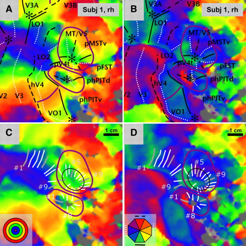
Eccentricity and polar angle maps in a single subject (subject 1, right hemisphere). Flat maps of the visual cortical region surrounding MT/V5, with eccentricity (A, C) and polar angle maps (B, D) superimposed. In A and B, the full and dashed black lines indicate lower and upper vertical meridians, the white dotted lines indicate horizontal meridians, the asterisks indicate central visual field, and the purple lines show positions of peripheral eccentricity ridges. In C and D, the white lines indicate the isopolar lines of the MT/V5 (n = 16) and phPIT (n = 8) clusters and the LO regions (n = 9). The light gray lines are isopolar lines corresponding to meridians in A and B, the numbers indicate their line index (5 and 9 for the MT/V5 cluster, 1 and 8 for the phPIT cluster and 1 and 9 for the LO regions), and the thin black line, the ellipses fitted to the isopolar lines. Scale bar, 1 cm. The insets show discrete color wheels for eccentricity and polar angle. Color progressions on the surfaces are continuous.
Figure 3.

Eccentricity and polar angle maps in MT/V5 and surrounding regions of subject 5, left hemisphere. The conventions are the same as in Figure 2.
The central representation of the MT/V5 cluster is located on the flat map at about the same dorsoventral level as the central confluence and is separated from LO2 and LO1 by an eccentricity ridge: a region of larger eccentricities separating the central confluence from the center representation in the MT/V5 cluster. This eccentricity ridge, which has already been noted in previous studies (Tootell and Hadjikhani, 2001), is present in all subjects, but is more extensive in some subjects (Fig. 3A) than in others (Fig. 2A) and is frequently part of an eccentricity circle surrounding the MT/V5 cluster (Fig. 3A). Another example of an eccentricity ridge in Figure 3A is that separating human area V4 (hV4) and VO1. Identification of the central representations of the MT/V5 cluster is crucial to recognizing the topographic organization of MT/V5. Indeed, Figures 2 and 3 show that a polar angle map consistent with a hemifield representation extends dorsally from the central representation of the MT/V5 cluster. Its lower vertical meridian (LVM) is located caudally (i.e., on the side of LO1–2) and the upper vertical meridian (UVM) rostrally, defining the borders of area MT/V5 (Georgieva et al., 2009; Pitzalis et al., 2010). These features are very similar to those of the monkey retinotopic map in which the center of the MT/V5 cluster is separated from V4d by an eccentricity ridge and the lower vertical meridian of the MT/V5 map is located caudally on the side toward V4d [Kolster et al. (2009), their Fig. 4].
Figure 4.

Polar angle plotted as a function of line index for the left (top) and right (bottom) hemispheres of each of the 10 subjects. The thin lines connect the average polar angle of each line. Red lines, Subject 1, rh; blue line, subject 5, lh; black lines, other hemispheres. The total number of nodes is indicated for each subject with the number of outliers in brackets.
In each of the 20 hemispheres, MT/V5 was bordered rostrally by another retinotopic region sharing the same central presentation as MT/V5 and containing a polar map, which is mirror-symmetric around the upper vertical meridian and shows a sign reversal (Sereno et al., 1995) at this level (Figs. 2B, 3B). These features are exactly those of MSTv in the monkey (Kolster et al., 2009); hence we consider this area the likely homolog of monkey MSTv, referring to it as putative MSTv (pMSTv). Next to pMSTv, there are indications of another map, symmetric around the lower vertical meridian, as clearly seen in Figure 3B and supplemental Figure S3B (available at www.jneurosci.org as supplemental material). This fits the description of FST in the monkey. We therefore refer to this region as pFST. Finally, in every hemisphere, MT/V5 was bordered on the caudal side by another retinotopic region in which the polar map is again mirror-symmetric, this time around the lower vertical meridian (Figs. 2B, 3B; supplemental Figs. S2B, S3B, available at www.jneurosci.org as supplemental material) and also shares the same central representation. This is similar to monkey V4t, which supposedly covers only the lower quadrant (Desimone and Ungerleider, 1986; Gattass et al., 1988), but in some of the hemispheres studied by Kolster et al. (2009) may have included a complete hemifield. Because in humans pV4t covers the complete hemifield, the MT/V5 cluster forms a complete circle and pV4t shares an upper vertical meridian representation at its border with pFST (Fig. 3B). In only 1 of the 20 hemispheres (subject 10, left hemisphere) was a small gap (∼7% of the full circle) present between the upper vertical representations in pV4t and pFST. Thus, the MT/V5 cluster includes two upper vertical meridians (Fig. 3B), a prominent one separating MT/V5 from pMSTv and a weaker one separating pV4t from pFST, and also two lower vertical meridians, again with a more pronounced one, separating MT/V5 from pV4t and a weaker one separating pMSTv from pFST.
Analysis of MT/V5 cluster using isopolar lines
To complement the visual analysis, we adapted a methodology introduced by Arcaro et al. (2009) using isopolar lines to analyze the MT/V5 cluster. These lines follow as closely as possible the polar angle progression while running approximately orthogonal to the eccentricity progression. This means that for the MT/V5 cluster they radiate from the central representation. They are indicated in C and D of Figures 2 and 3, and supplemental Figures S2 and S3 (available at www.jneurosci.org as supplemental material). It can be seen that the spacing of the lines adapts to the abruptness of the color changes, being close when the color is changing rapidly and more widely spaced when the polar angle varies slowly. The results of this analysis applied to the MT/V5 cluster are shown in Figure 4: the polar angles (in radians) of all the nodes along a line are plotted as a function of the position of that line indicated by its index number (1 through 16) with line 1 plotted twice. The thin line connects the average polar angle of each line. For each subject, the data for the left and right hemispheres are plotted with opposite signs of polar angle, where a polar angle of zero corresponds to the LVM and an angle of ±3.14 to the UVM. In this figure, the red curve for subject 1 corresponds to Figure 2, and the blue curve for subject 5 corresponds to Figure 3. The two other curves from these same two subjects correspond to supplemental Figures S2 and S3 (available at www.jneurosci.org as supplemental material). For both these subjects, the polar angle moves from LVM to UVM between lines 1 and 5, then back to LVM between lines 5 and 9, up again between lines 9 and 13, and then again down between lines 13 and 1, producing a characteristic “W” pattern for the right hemisphere and an “inverted W” for the left hemisphere. Notice that the degree of scatter in polar angles along any given line is generally small, except for lines close to 13. Nonetheless, the mean pattern of polar angle variation remains very clear in all four hemispheres, successively defining four hemifields corresponding to MT/V5, pMST, pFST, and pV4t.
The same pattern was obtained in the eight other subjects, also shown in Figure 4. For each subject, the total number of nodes sampled along the 32 lines is indicated, as is the number of outliers rejected (those more than 0.3 radians into the ipsilateral field). The total number of nodes per subject ranged from 287 to 381 with an average close to 320, corresponding to 10 nodes per line. For most subjects, the number of outliers was zero or one, although in two subjects the proportion of outliers reached 2% of the nodes, and in one subject, 3%. The small numbers of such outliers, together with the limited scatter in the polar angle along most lines, clearly indicate the quality of the polar angle maps. In 9 of 10 right hemispheres, the W pattern indicating four complete hemifields within the cluster is clearly discernable, the exception being subject 7 for whom the reversal between pMSTv and pFST is shallow. The same applies to the left hemispheres where the only exception was subject 4 whose reversal between pFST and pV4t is shallow. This subject whose map was shown in the study by Georgieva et al. (2009) was retested with very similar results (supplemental Fig. S4, available at www.jneurosci.org as supplemental material).
The average results from individual left and right hemispheres, corresponding to the thin lines in Figure 4, are plotted in Figure 5A. The average over all the hemispheres shows that, although the W and inverted W patterns are very clear, the polar angle falls short of the expected values by nearly a radian at most reversals, thus reducing the total observed variation in the average polar angle across the different hemifields to little more than 1 radian, as reported for areas PH1 and PH2 in the study by Arcaro et al. (2009). A comparison of individual data with the population average indicates that the two hemispheres chosen for illustration in Figures 2 and 3 are close to this average, making them very representative.
Figure 5.

Average polar angle of all subjects plotted as a function of line index for the MT/V5 cluster (A), the phPIT cluster (B), and the LO1/2 regions (C) in left (LH) and right hemisphere (RH). Gray dots, Subject averages; black lines, grand averages; red and blue circles, data of subject 1, right hemisphere, and 5, left hemisphere, respectively.
One reason that the polar angle undershoots the expected values in Figure 5 may be that the polar angle is better defined near the end of the isopolar lines, away from the center where some smearing of the polar angle is bound to occur (see Materials and Methods). Therefore, we complemented the isopolar line analysis with one used by Kolster et al. (2009), mapping polar angle along an ellipse fitted to the middle of the isopolar lines (thin black lines in Figs. 2, 3; supplemental Figs. S2, S3, available at www.jneurosci.org as supplemental material). This procedure complements the isopolar analysis by also sampling in between the isopolar lines. The individual and average results are shown in Figure 6A. The average across hemispheres now clearly shows larger deflections in the polar angle in all the hemifields: the largest variation, close to 2 radians, is observed in right and left MT/V5, right pV4t, and left pMSTv. The smallest variation in polar angle, a little under 1.5 radians, was observed in right and left pFST. Thus, there is a tendency for the polar angle reversals to deviate most from the predicted value at the pMSTv/pFST border. This is expected since, in the monkey, the neurons of these two areas have the largest RFs (Desimone and Ungerleider, 1986). This effect will also be magnified because the cortical area is small. Despite the smaller than expected polar angles at the reversals, the correlation of the observed polar angle curves with the theoretical W or inverted W pattern was high. For the average curves, the correlation was 0.92 for the left hemisphere and 0.85 for the right hemisphere. For individual subjects, correlation ranged from 0.62 to 0.90 in the right hemisphere and from 0.66 to 0.91 in the left hemisphere. This extensive analysis confirms that the MT/V5 cluster includes four hemifields sharing a central representation and the polar maps of which are all mirror-symmetric with their neighbors.
Figure 6.

A, Polar angle plotted as a function of position along the ellipses fitted to the isopolar lines in the MT/V5 cluster. Gray dots, Individual subjects; red circles, subject 1, rh; blue circles, subject 5, lh; black line, average across subjects. LH, Left hemisphere; RH, right hemisphere. B, Eccentricity in the visual field plotted as a function of distance along the cortex from center representation in MT/V5, pMST, pFST, and pV4t of left (blue) and right (red) hemispheres. The dashed line represents an approximate progression of eccentricity as a function of cortical distance for MT/V5 of both hemispheres.
General features of the MT/V5 cluster
The mean Talairach [Montreal Neurological Institute (MNI)] coordinates of left and right MT/V5 were as follows: −48, −75, 8, and 46, −78, 6 (Table 1). Extreme values were 134 mm2 [left hemisphere (lh), subject 10] and 339 mm2 [right hemisphere (rh), subject 4]. These latter values corresponded to 78 and 156 voxels, respectively, and to 172 and 383 nodes, respectively (see Materials and Methods). The mean surface area values are similar to those reported for MT/V5 as defined anatomically (228 mm2) (Tootell and Taylor, 1995). The surface area of V1 was quite similar in the two hemispheres: 1147 mm2 for left and 1140 mm2 for right V1. Hence MT/V5 occupies between 17 and 23% the surface of V1 and is approximately the same size as VO1, which amounts to 22% of V1 according to Arcaro et al. (2009). Area MT/V5 is the only area in the cluster with a significant size difference between hemispheres. For the other three areas, surfaces were more or less equal in the two hemispheres. The left–right asymmetry of the MT/V5 surface area proved significant: a two-way ANOVA with hemisphere and gender as factors yielded a significant effect of hemisphere (F(1,16) = 7.43; p < 0.02) but no effect of gender and no interaction.
Table 1.
Average Talairach coordinates (MNI) of the center of areas in MT/V5 and phPIT cluster and the LO1/2 areas in the left and right hemispheres
| Area | LH |
RH |
||||
|---|---|---|---|---|---|---|
| X | Y | Z | X | Y | Z | |
| MT/V5 | −48 | −75 | 8 | 46 | −78 | 6 |
| pMSTv | −45 | −67 | 6 | 44 | −70 | 5 |
| pFST | −46 | −72 | 0 | 46 | −74 | −4 |
| pV4t | −48 | −78 | 3 | 47 | −81 | −2 |
| phPITd | −40 | −85 | −6 | 42 | −85 | −9 |
| phPITv | −39 | −84 | −8 | 40 | −84 | −11 |
| LO1 | −36 | −90 | 4 | 36 | −92 | 3 |
| LO2 | −42 | −89 | −2 | 40 | −91 | −3 |
For area pMST, the mean coordinates were −45, −67, 6, and 44, −70, 5 (Table 1). Surface areas were on average 201 and 178 mm2 (Table 2). This corresponds to 17% of V1. The mean coordinates of pFST were −456, −72, 0, and 46, −74, −4 (Table 1), and surface areas were 145 and 119 mm2 (Table 2). Thus, pFST is a small area, amounting to 12% of V1. Finally, coordinates of pV4t were −48, −78, 3, and 47, 81, −2 (Table 1). Mean surface areas were 103 and 110 mm2 (Table 2), representing only 9% of V1. In total, the surface area of the entire MT/V5 cluster amounts to 58% of that of V1.
Table 2.
Surface area of areas in MT/V5 and phPIT cluster and the LO1/2 areas in the left and right hemispheres
| Area | LH (mm2) | RH (mm2) |
|---|---|---|
| MT/V5 | 202 ± 55 | 265 ± 71 |
| pMSTv | 201 ± 61 | 178 ± 89 |
| pFST | 145 ± 62 | 119 ± 49 |
| pV4t | 103 ± 30 | 110 ± 33 |
| phPITd | 192 ± 102 | 142 ± 40 |
| pPITv | 200 ± 96 | 175 ± 108 |
| LO1 | 350 ± 147 | 325 ± 99 |
| LO2 | 317 ± 117 | 202 ± 63 |
Values are expressed as average ± SD.
Figure 6B plots eccentricity in the visual field along the horizontal meridian as a function of cortical distance from the center for the four members of the MT/V5 cluster in the left and right hemispheres. Data points were included in these average curves if at least five subjects contributed to a given cortical distance. In MT/V5, eccentricities between 1 and 4° are represented along 12 mm cortex, corresponding to a magnification factor of 4 mm per visual degree. In V1, the magnification for those eccentricities would be approximately double according to Larsson and Heeger (2006) and Qiu et al. (2006). This fits with the ratio of the surface areas of MT/V5 and V1 (Table 2), as √5 equals 2.2. In the other three areas, cortical magnification is slightly lower, especially in pV4t. In this area, eccentricities from 1 to 4° are represented by a distance of 9 mm on the cortex, yielding a linear MF of 3 mm/deg. This again fits with the ratio of the surface areas of MT/V5 and V4t (Table 2), since √2 equals 1.4 and we expect a MF of 4/1.4 = 2.9, very close to the 3 mm/deg estimated from Figure 6B.
Retinotopic organization of neighboring areas: LO and phPIT regions
Below the MT/V5 cluster, there is another central representation that is generally surrounded by an eccentricity ring (Figs. 2, 3). The polar angle map indicates a representation of upper and lower vertical meridians that is consistent with two hemifield representations, one dorsal and one ventral, sharing a central representation and the upper and lower vertical meridians (Figs. 2B, 3B; supplemental Figs. S2B, S3B, available at www.jneurosci.org as supplemental material). In the monkey (Kolster et al., 2009), a retinotopic map, PITd, has been described below the MT/V5 cluster (Fig. 1) with an overall organization similar to the dorsal region, which in humans also abuts the MT/V5 cluster. Felleman and Van Essen (1991) have proposed that the posterior part of inferotemporal cortex, corresponding to architectonic temporal occipital area (TEO), should be split into two regions, which they labeled PITd and PITv. Kolster et al. (2009), in suggesting that the retinotopic region ventral to the cluster was PITd, assumed that there was a second more ventral portion that was also retinotopically organized. There is evidence for such a ventral region (Gattass et al., 2005), but it was labeled TEO. We propose that the two human regions in the cluster below the MT/V5 cluster correspond to monkey PITd and PITv. Since there was evidence in the study by Kolster et al. (2009) for an eccentricity ridge between the MT/V5 cluster and PITd but no indication for an isolated PIT cluster, it is possible that the exact retinotopic organization of these PIT regions is somewhat different in humans and in monkeys. For that reason, we have labeled them putative human PIT dorsal and ventral (phPITd and phPITv).
To confirm the existence of two cortical areas in the phPIT cluster, we performed an isopolar line analysis similar to that performed for the MT/V5 cluster, placing eight isopolar lines around the center of the cluster (Figs. 2C, 3C; supplemental S2C, S3C, available at www.jneurosci.org as supplemental material). The polar angle-line index curves for the individual hemispheres are plotted in supplemental Figure S5 (available at www.jneurosci.org as supplemental material). Again, the maps shown in Figures 2 and 3 correspond to the red and the blue curves, respectively. The number of nodes per subject ranges from 90 to 120, indicating that each isopolar line included six to eight nodes. The number of outliers is again small except in subjects 3 and 4, for whom it reached 8 or 9%. Also, the scatter in the polar angle values is small for most lines, underscoring the quality of the polar angle maps in this region. In all subjects, a typical “inverted V” or “V” pattern was discernable in the left and right hemispheres, respectively, indicating a single reversal around the lower vertical meridian at line 5, located near the rostral end of the cluster. The average curves for the population are shown in Figure 5B and confirm that two hemifields are present in the cluster corresponding to areas phPITd and phPITv. Interestingly, the total variation in the polar angle in these two hemifields is slightly greater than in the hemifields of the MT/V5 cluster (Fig. 5, compare A, B).
The mean Talairach (MNI) coordinates of left and right phPITd were −40, −85, −6, and 42, −85, −9 (Table 1). Those of phPITv were almost identical: −39, −84, −8, and 40, −84, −10. Thus, these areas can be dissociated only by explicit retinotopic mapping. The surface area measured 192 and 142 mm2 for left and right phPITd, compared with 200 and 175 mm2 for phPITv (Table 2). This amounts to 15 and 16% of the V1 surface area, respectively.
Finally, the two remaining neighbors of MT/V5 in the human are LO1 and LO2, which have been described previously (Larsson and Heeger, 2006; Georgieva et al., 2009). These retinotopic data are consistent with the view that, in humans, LO1–2 and hV4, respectively, occupy the positions of V4d and V4v in the monkey (Larsson and Heeger, 2006; Wandell et al., 2007). There is disagreement, however, about the exact organization in this region of cortex (Hansen et al., 2007). In addition, although we adhere to the definition provided by Larsson and Heeger (2006) for LO1 and LO2, these areas might be affected by the modification of the retinotopic organization we proposed for the V3A complex (Georgieva et al., 2009), restoring V3A to the location described by Tootell et al. (1997). Therefore, we also performed an isopolar lines analysis for the pair LO1–LO2. We did not include hV4 in this analysis, because this has recently been done by Arcaro et al. (2009). We defined nine isopolar lines spanning the range of polar angle in LO1 and LO2 and centered on the central confluence in which LO1 and LO2 participate (Figs. 2A, 3A). The results are shown in supplemental Figure S6 (available at www.jneurosci.org as supplemental material), following exactly the same conventions as in supplemental Figure S5 (available at www.jneurosci.org as supplemental material). The number of nodes ranged from 184 to 366 per subject, indicating that each line included an average of 10 and 20 nodes. The scatter in the polar angle is generally small for most of the isopolar lines, and in most subjects the fraction of outliers is <1%. In two subjects, this fraction did reach 10%, however. Thus, in general, the polar maps were of good quality in this region of the cortex. As for the phPIT pair, the curves in most subjects followed a V (right hemisphere) or inverted V pattern (left hemisphere), typical of two cortical areas joined by a common upper vertical meridian, as initially described by Larsson and Heeger (2006). In only two hemispheres, the left hemispheres of subjects 5 and 11, was the reversal shallow. The average curves for the population are shown in Figure 5C. The amplitude of the deflection in polar angle was more or less similar to that of the phPIT regions, with a minor restriction for the left hemisphere, in keeping with the two shallow reversals noticed in the single subjects. This compares favorably with the results of Larsson and Heeger (2006), who reported a polar angle variation of 1.5 radians in LO1/LO2 after fitting to an atlas. Notice that the pattern shown by the polar angles is exactly the opposite of that obtained for phPIT (Fig. 5, compare C, B): LO1 and LO2 areas are mirror-symmetric around the upper vertical meridian, whereas in fact the phPIT regions are symmetric around the whole vertical meridian. Indeed, in Figure 5B, line 1 is plotted twice, whereas in Figure 5C lines 1 and 9 are quite distant from one another. This analysis confirms the existence of two hemifield representations located between dorsal V3 and the MT/V5 cluster in humans. It is worth noting that there is no gap in the retinotopic maps between LO1/2 and the MT/V5 cluster (Figs. 2, 3; supplemental Figs. S2, S3, available at www.jneurosci.org as supplemental material). It is mainly areas V4t and phPITd/v that fill the space between LO1/2, hV4, and the MT/V5 cluster, and these areas have not previously been identified. Also, it should be noted that both the two LO regions and hV4 participate in the central confluence, as V4 does in the monkey.
Whereas areas LO1 and LO2 share the central confluence with areas V1–3, the MT/V5 and phPIT clusters have their own representation of the central visual field. This raises a question regarding the geometrical relationships between these areas in the flat maps. To investigate these relationships, we considered the HM in LO2 and MT/V5 and the VM in phPIT, computing the angles they make with a common reference: the LVM that constitutes the anterior border of V3d (Fig. 7A). These angles are compared in the left and right hemispheres in the graph of Figure 7B. This graph shows that most angles cluster close to the diagonal, indicating that the overall geometry is similar in the two hemispheres. The HM of MT/V5 makes an angle of approximately −30° with the UVM in V3d in both hemispheres. However, the angle of the HM in LO2 is ∼60 and 80° in the left and right hemispheres. This means that these two HMs run approximately orthogonal to each other in the flat maps. This is remarkable since Amano et al. (2009) assumed that LO2 and temporal occipital 1 (TO1), which they considered a possible homolog of MT/V5, were parallel in the flat maps. The VM in phPIT makes an angle of ∼90–110° with the UVM in V3d, which means that it has an angle of ∼30° with the HM of LO2: this fits with the fact that the phPIT cluster is wedged between LO2 and hV4.
Figure 7.

A, Schematic representation of HM and VMs in areas LO1, LO2, MT/V5, and phPITd and phPITv, and definition of the angles α, β, and γ with respect to the anterior border of V3d. B, The angles α, β, and γ of the left hemisphere plotted as a function of the same angles in the right hemisphere.
The mean Talairach (MNI) coordinates for left and right LO1 were −36, −90, 4, and 36, −92, 3, and −42, −89, −2, and 40, −91, −3, for left and right LO2 (Table 1). The surface area measured 350 and 325 mm2 for left and right LO1, corresponding to 29% of V1. For LO2, surface area was 317 and 202 mm2 for left and right LO2, corresponding to an average of 23% of V1, values very similar to those of Larsson and Heeger (2006), who reported figures of 28 and 29% of V1 for LO1 and LO2, respectively. Thus, LO1 and LO2 are larger than any of the areas in the MT/V5 or phPIT clusters. The surface area of left LO2 was larger than that of right LO2 (Table 2). A two-way ANOVA with hemisphere and gender as factors yielded a significant effect of hemisphere (F(1,16) = 9.80; p < 0.01), no effect of gender but a significant interaction (F(1,16) = 6.79; p < 0.02), the effect being larger in male than in female subjects. LO2 is located directly caudal to MT/V5, and the opposite asymmetry observed in the two hemispheres suggests that an increase in one area is compensated for by a decrease of the other. Plotting the surface area of LO2 as a function of that of MT/V5 in all 20 hemispheres indeed yielded a significant negative correlation (r = −0.47; p < 0.05).
Retinotopic stimulus signal strength
To evaluate the strength of the MR signals evoked by the retinotopic stimuli we plotted MR signals as a function of temporal frequency for the different areas. The stimuli evoke a temporal waveform in visual cortex voxels, which we average over the four runs collected in each subject for either the expanding rings or the rotating wedges. These data were Fourier-transformed and normalized, and the spectra averaged, first within individual areas and then over hemispheres (see Materials and Methods). This resulted in two average spectra for each area: one for the polar mapping and one for the eccentricity mapping (Fig. 8). Given the normalization, amplitude is indicated as percentage of mean MR activity, after subtraction of baseline. The abscissa indicates temporal frequency in number of cycles per 256 s. Converting amplitude to percentage signal change becomes complex when amplitudes at several temporal frequencies are significant and the noise level is nonzero, as is the case in our data. The frequencies at which the activity is significantly different from the noise level are indicated by the colored asterisks in Figure 8. Spectra of areas V1 and hV4 are indicated for reference. In each of the eight areas of interest, the activity at the basic stimulus frequency (4 cycles) was significant for both the polar mapping (Fig. 8A) and eccentricity mapping (Fig. 8B), even though the amplitudes were relatively small beyond hV4. These amplitudes were all very similar, lying between 0.15 and 0.2%, in MT/ V5, pV4t, the two phPIT regions, and the two LO regions. In pMSTv and pFST, they were only slightly smaller, ranging between 0.15 and 0.1%. The results for the eccentricity mapping were similar but with slightly weaker amplitudes than those for the polar angle mapping, a tendency also noticed by Arcaro et al. (2009). Given the larger number of runs (10 instead of 4) and cycles (6 instead of 4), we expected amplitudes only one-half as large as those obtained by Arcaro et al. (2009).Consequently, our results for the MT/V5 cluster, the phPIT, and LO regions fall between those obtained by Arcaro et al. (2009) for PH1 and PH2.
Figure 8.

Histograms plotting amplitude of the different temporal frequency components for polar maps (A) and eccentricity maps (B) in V1, MT/V5, pMSTv, pFST, pV4t, hV4, LO1, LO2, phPITv, and phPITd. The baseline has been subtracted (see Materials and Methods). The envelope of the amplitudes centered at zero (gray line) is the Fourier transform of the temporal waveform of a single cycle. The vertical bars indicate SE across hemispheres; the colored asterisks indicate significant components: green, basic stimulus frequency; orange, harmonics of the basic frequency.
The number of temporal frequencies that reach significance informs us about the temporal waveform in a given area. In V1, five temporal frequencies reached significance including the fourth harmonic (20 cycles) of the basic temporal frequency. This corresponds to a narrow temporal waveform, reflecting the presence of small RFs with little scatter. In MST, however, only the basic temporal frequency of 4 cycles reached significance. This indicates a broad temporal waveform close to a sinusoid, indicative of large RFs with considerable scatter. The duration of the average temporal waveform at 3.25° eccentricity, derived from the envelope to the spectrograms of the different areas (Fig. 8), is plotted as the FWHM for the radial and azimuthal directions in Figure 9A. In most areas of the MT/V5 cluster, the duration exceeds 40 s, especially in the polar direction. This underscores the need for long stimulus cycles, in particular for the rotating wedges. Furthermore, the radial width of MT/V5 was intermediate between that of hV4 and V1, a sequence similar to what was observed in the monkey (Kolster et al., 2009).
Figure 9.

FWHM of the hemodynamic response signal in the time domain and corresponding pRF sizes of visual areas, based on approximations of the harmonic spectra (Fig. 8) by Gaussian functions. The data in radial and azimuthal directions are derived from the expanding annulus and rotating wedge measurements, respectively. A, Radial versus azimuthal FWHM of the HR signals (in seconds). The dark and light gray boxes indicate the size of the stimulus and FWHM of a typical HR function, respectively. The thin gray diagonal line indicates points of equal radial and azimuthal values. B, Radial versus azimuthal widths of the pRFs (in degrees). The thin gray line indicates points of equal radial and azimuthal values. The dashed amber line represents a straight line through the origin fitted to the values of areas within the MT/V5 cluster.
Converting the waveform duration to spatial dimensions yields the mean width in the radial and azimuthal directions of the population RF at 3.25° eccentricity (Fig. 9B). The pRF is compressed in the radial direction to the same degree throughout the MT/V5 cluster. In monkey MT/V5, RFs are compressed in the direction orthogonal to the preferred direction (Raiguel et al., 1995), and for more peripheral RFs the preferred directions exhibit a radial bias (Albright, 1989). The present results suggest that this bias extends to more central fields in human MT/V5, perhaps reflecting changes in habitat, and/or is detected at smaller eccentricities by the fMRI. The pRFs in hV4 and V1 are close to circular-symmetric, which is consistent with the results of Motter (2009). The population RF primarily reflects the mean width of the RFs at a given eccentricity and their scatter. Hubel and Wiesel (1974) measured the scatter of RF positions in the superficial layers of V1 and found the width of the population RF (their Fig. 7) to equal approximately three times the mean RF width. Unfortunately, although there are clear indications that scatter increases across areas together with mean RF size (Desimone and Ungerleider, 1986), little or no explicit measures of scatter in extrastriate areas are available. RF width depends not only on eccentricity but also on laminar position (Raiguel et al., 1995; Gur et al., 2005), on the stimuli used to map the RF, and on use of quantitative versus qualitative techniques, the latter usually underestimating the RF size. Using the estimate of the pRF provided by Hubel and Wiesel (1974), we expect a pRF at 3.25° eccentricity of 1.15°. Quantitative measures are similar for these layers (Gur et al., 2005), and the stimuli (small light bars) are relatively similar to the flickering checkerboards used here; hence given the larger size of human V1 (a factor of 2), we would expect a pRF in human V1 of 1.15°/√2, which equals 0.8°. We observed a slightly larger value (1.2°), which might be attributable to the fact that RFs in deeper layers, which blood oxygen level dependence (BOLD) also samples, are larger than in layers 2 and 3. Other factors include the relatively wide range of eccentricities included in the average pRF, the interaction between RF size variance with position scatter, and small measurement errors.
The RF width in MT/V5 measured quantitatively (Raiguel et al., 1995) averages 5.5° at 3.25° eccentricity, a value not very different from the RF size measured by Tanaka et al. (1993) with handheld stimuli (5.1°). Using the same scatter size as estimated in V1 (Hubel and Wiesel, 1974), we expect a pRF in the monkey of 16.5°. The results of Kolster et al. (2009) indicate that this is likely an overestimation, perhaps because scatter is smaller in MT/V5 or RF sizes are more homogeneous. From the magnification in human MT/V5, which is approximately three times greater than in monkey (Maunsell and Van Essen 1987), we expect a human pRF of 5.5°, very close to the 6° we actually obtained (Fig. 9B). This match should be interpreted with care as we had to make many assumptions, which will have to be verified by performing parallel recording and imaging experiments in monkeys and by using exactly the same procedures in human and monkey imaging experiments. The pRF of pMSTv is larger than that of MT/V5, as we would expect based on the mean RF width at 3.25° in the equivalent monkey areas. The proportion of these pRFs, however, is smaller than expected from the monkey RF sizes, as Tanaka et al. (1993) report a 5.5-fold larger mean RF for MSTv compared with MT/V5, and Desimone and Ungerleider (1986), a 4.7-fold ratio. However, the mean RF size for V4t was approximately the same as for MT/V5 in the Desimone and Ungerleider (1986) study, yet the pRF of pV4t is smaller than that of MT/V5 (Fig. 9B). Similarly, the mean RF size of FST was 3.4-fold that of MT/V5 according to Desimone and Ungerleider (1986) and the pRF of pFST is actually smaller than that of MT/V5. This suggests that, proportionally, the three other areas of the human MT/V5 cluster have gained more in magnification than MT/V5 itself. Alternatively or additionally, it may be that the scatter is smaller in these human areas than in their monkey counterparts.
Visual field representations in MT/V5 and surrounding regions
For each area and subject, we calculated the number of surface nodes for which both eccentricity and polar angle measurements were available. The average numbers per area in left and right hemispheres are indicated in Table 3. The location of each node with respect to eccentricity and polar angle was then plotted for each area and subject, as shown for the group of subjects in Figure 10. The blue dots denote nodes from the left hemisphere, and the red dots nodes from the right hemisphere. In addition to the eight areas mapped in detail in the present study, we have also included V1 and hV4 for reference. All areas represented the contralateral visual field almost exclusively. In V1, the vast majority (95 and 96%) of the nodes were located in the contralateral hemisphere, thus replicating previous results (Larsson and Heeger, 2006; Arcaro et al., 2009). The same was true for the areas of the MT/V5 cluster, and also to a slightly lesser degree for LO1/2 and the phPIT regions (Table 3). The few nodes located in the ipsilateral field include the small number of outliers that were excluded in the isopolar line analysis (Fig. 4; supplemental Figs. S5, S6, available at www.jneurosci.org as supplemental material).
Table 3.
Number of nodes and percentage contralateral nodes in different cortical areas of left and right hemisphere
| Area | Nodes |
% Contralateral |
||
|---|---|---|---|---|
| LH | RH | LH | RH | |
| V1 | 1536 ± 389 | 1435 ± 329 | 95 ± 6 | 96 ± 4 |
| hV4 | 652 ± 219 | 681 ± 137 | 98 ± 2 | 98 ± 3 |
| MT/V5 | 231 ± 81 | 315 ± 83 | 96 ± 10 | 97 ± 5 |
| pMST | 225 ± 95 | 209 ± 113 | 99 ± 3 | 96 ± 7 |
| pFST | 164 ± 83 | 132 ± 59 | 95 ± 8 | 99 ± 1 |
| pV4t | 109 ± 36 | 121 ± 36 | 95 ± 11 | 96 ± 9 |
| LO1 | 446 ± 182 | 406 ± 127 | 93 ± 9 | 97 ± 5 |
| LO2 | 424 ± 146 | 250 ± 82 | 90 ± 12 | 96 ± 8 |
| phPITv | 238 ± 127 | 146 ± 51 | 92 ± 9 | 97 ± 9 |
| phPITd | 220 ± 138 | 163 ± 53 | 90 ± 12 | 97 ± 6 |
Values are expressed as average ± SD.
Figure 10.

Visual field representations in areas V1, MT/V5, pMSTv, pFST, pV4t, hV4, LO1, LO2, phPITv, and phPITd. Red dots, Nodes in right hemisphere (RH); blue dots, nodes in left hemisphere (LH). UVF, Upper visual field; LVF, lower visual field. The visual field representation is subdivided into three sectors corresponding to eccentricities smaller than 2.5°, between 2.5 and 5°, and between 5 and 7.5°. The data plotted in the graphs represent the data that were used in the functional grid analysis.
The data were further evaluated for upper field versus lower field representation (averaging over contralateral nodes of the left and right hemispheres). Table 4 lists the percentage nodes that represented the upper field. If both quadrants are represented equally, this percentage should be 50%. The percentage was close to 50% in V1, in agreement with Arcaro et al. (2009), and also in the areas of the MT/V5 cluster and the two phPIT regions. Thus, the hemifield was represented uniformly in these regions, confirming the isopolar line analysis. However, in hV4, the percentage reached 65%, although not significantly different from 50% after correction for multiple comparisons (Table 4), consistent with Arcaro et al. (2009). However, in LO1 and LO2, the percentages were 29 and 30%, significantly different from 50% after correction for multiple comparisons, indicating a strong bias toward the lower quadrant (Table 4). Larsson and Heeger (2006) also reported a bias favoring the lower quadrant in LO1/2 and the upper quadrant in hV4.
Table 4.
Percentage upper quadrant nodes, t and p values of comparison with 50% in different cortical areas
| Areas | % UVF | t | p |
|---|---|---|---|
| V1 | 44 ± 3 | −2.02 | 0.075 |
| hV4 | 64 ± 4 | 4.07 | 0.028 |
| MT/V5 | 44 ± 6 | −1.06 | 0.315 |
| pMSTv | 53 ± 7 | 0.47 | 0.652 |
| pFST | 42 ± 7 | −1.18 | 0.267 |
| pV4t | 40 ± 6 | −1.69 | 0.125 |
| LO1 | 29 ± 5* | −3.96 | 0.003 |
| LO2 | 30 ± 4* | −4.43 | 0.002 |
| phPITv | 42 ± 6 | −1.34 | 0.212 |
| phPITd | 39 ± 6 | −1.68 | 0.127 |
Values are expressed as average ± SD.
*Significant after correction for 10 comparisons.
Location of the MT/V5 retinotopic map with respect to anatomical and functional landmarks
A classical anatomical landmark is the gyral and sulcal pattern. Here, too, the individual variability is considerable. Figure 11 shows the location of MT/V5 and surrounding regions plotted on partially inflated hemispheres of three subjects. Figure 11, B and D, corresponds to the flat maps of Figures 2 and 3. The location of MT/V5 can be similar in the two hemispheres of a subject, as in subject 10, or rather different, as in subject 1. Generally, MT/V5 is associated with the posterior bank of the ascending branch of the inferior temporal sulcus (ITS) (subjects 3 and 10, lh), also referred to as anterior occipital sulcus (AOS) (Malikovic et al., 2007), but it can also be located in the upper bank of the inferior occipital sulcus (IOS) (subject 5 and 10, rh), on the gyral surface in between AOS and IOS (subject 1, lh) or even in the upper bank of LOS when this sulcus is located ventrally (subject 1, rh). Furthermore, MT/V5 is generally located rostrally relative to LO1/2, but in some hemispheres it is wedged between LO2 and phPIT (subject 1, rh), resulting in a more posterior position. However, area LO1 is associated relatively frequently with the lower bank of the LOS (Fig. 11A,C,D,F).
Figure 11.

Localization of MT/V5 (brown), pMSTv (orange), pFST (amber), pV4t (yellow), LO1 (dark green), LO2 (light green), and phPITd (turquoise) and phPITv (olive) on the inflated left and right hemispheres of subject 1 (A, B), left hemisphere of subject 3 (C), right hemisphere of subject 5 (D), and the two hemispheres of subject 10 (E, F). Purple line, Eccentricity ridge separating MT/V5 cluster from central confluence.
Supplemental Figure S7 (available at www.jneurosci.org as supplemental material) plots the sulcal index (see Materials and Methods) averaged across hemispheres for MT/V5 and its neighbors. Although the average value for V1, shown for reference, is negative, indicating a location on the gyrus, the sulcal index became less negative with increasing eccentricity in V1 corresponding to the known anatomical location of V1 (Hinds et al., 2009). The average sulcal index for MT/V5 is close to zero, indicating that it is located most often in the banks of sulci, mostly the AOS or the IOS. In contrast, the index of pMSTv and pFST is clearly positive, indicating that it is generally located more in the depth of those sulci, as was the case in most of the hemispheres of Figure 11.The sulcal index is also close to zero for LO1 corresponding to its location in a bank, generally that of LOS. Indices of LO2 and phPIT regions are on average negative, also corresponding to a location on gyri, either between LOS and IOS for LO2, or between IOS and OTS for the phPIT regions.
An important functional landmark with which to locate MT/V5 is the motion complex as provided by a localizer in which a moving stimulus is contrasted to the same, but stationary, pattern. Currently, human MT/V5+ is identified through its response to this localizer, which is typically located near the ITS/LOS landmark. Figure 12 plots the relationship between the retinotopic maps and the ML response defined at p < 0.05, familywise error (FWE) corrected, level for the two of the eight subjects (subjects 1 and 4) with whom the motion localizer was tested. In general, the localizer activates the MT/V5 cluster and also V3A, but avoids phPIT+ and LO1–2. In some subjects, an occasional activation of LO1–2 or even phPIT+ can be seen, and conversely MT/V5 itself can show but little motion response at that threshold. Figure 12 also shows that the LO localizer generally activates LO2, the phPIT complex and the ventral regions of the MT/V5 cluster (pV4t and pFST). But occasionally its activation extends into the whole of the MT/V5 cluster. Across all subjects, the cortical surface activated by the motion localizer at the ITS/IOS confluence is rather variable: its coefficient of variation is 49% compared with 33% for the surface of MT/V5. Importantly, retinotopic MT/V5 makes up a relatively small portion of the motion localizer activation, averaging only 16 and 20% for left and right hemispheres, respectively (Table 5). In fact, pMSTv constitutes a larger fraction of the ML, 24–30%, whereas pFST and pV4t represent only 12–22 and 8–9%, respectively. In total, the entire MT/V5 cluster constitutes 70% of the motion localizer activation area. This is not surprising since the monkey cortex possesses a second set of motion-sensitive regions beyond the MT/V5 cluster, such as MSTd, and it is likely that their homologs also contribute to the motion localizer activation.
Figure 12.

Flat map of cortex surrounding MT/V5 indicating the voxels significantly (p < 0.05, FWE corrected) activated by the motion localizer (A, C) and the two-dimensional shape (LO) localizer (B, D) in yellow (blue indicates voxels significant in the opposite subtraction). A, B, Right hemisphere (rh) of subject 1. C, D, Left hemisphere (lh) of subject 4.
Table 5.
Fraction of ML covered by areas of MT/V5 cluster
| Area | LH | RH |
|---|---|---|
| MT/V5 | 0.16 ± 0.14 | 0.20 ± 0.13 |
| pMSTv | 0.30 ± 0.26 | 0.24 ± 0.10 |
| pFST | 0.12 ± 0.14 | 0.22 ± 0.13 |
| pV4t | 0.09 ± 0.09 | 0.08 ± 0.07 |
| Total | 0.67 ± 0.28 | 0.74 ± 0.27 |
The variability of the fraction of the ML represented by MT/V5 (Table 5) implies that, in some subjects, this fraction is zero. This does not mean that MT/V5 does not respond to motion, but that no voxel in MT/V5 reaches the stringent p < 0.05 corrected level with two runs of the localizer sampled. This reflects the intersubject variability in the motion sensitivity of MT/V5. As shown in supplemental Figure S8 (available at www.jneurosci.org as supplemental material), the level of activation equaled or exceeded the mean in most of the eight subjects tested, but in one subject (subject 11) the level was clearly below the mean, indicating a small but significant motion response. In this subject, very few voxels reached significance (p < 0.05, FWE corrected) within the motion localizer. It is therefore important to distinguish the mere presence of a motion response in MT/V5 and an activation strong enough to reach significance at the voxel level. Whereas the former was true in all subjects, the latter was occasionally not verified. Hence relying solely on the ML to derive the cortical region that corresponds to MT/V5 (Huk et al., 2002) may produce spurious results.
Functional grid analysis; the effect of eccentricity
For the analysis of the functional tests, we made use of the association between the functional test data and the retinotopic data that was defined for each visual area in each subject based on the surface nodes (see Materials and Methods). This method allows for an analysis of unsmoothed functional test data at the group level by correlating similar points in the cortex of individual subjects by means of their representations in the visual field (Brefczynski-Lewis et al., 2009) without anatomical registration between subjects (Fig. 13A). Figure 13B plots the percentage BOLD signal change induced by random texture motion, relative to a static reference, as a function of eccentricity for the eight areas under study, with V1 indicated for reference. The diameter of the motion localizer stimuli was 7°, corresponding to a radius of 3.5°. The data were integrated in 1° steps from 0.5 to 7.5° of eccentricity and over the full range of polar angles, reflecting the symmetrical shape of the localizer. As expected (Zeki et al., 1991; Tootell et al., 1995), V1 gave intermediate responses to the moving stimulus, between 0.5 and 1% change in MR signal strength above static, over the three bins corresponding to the extent of the stimulus. In all four regions of the MT/V5 cluster, responses over these three bins were stronger. In LO2 and the two phPIT regions, responses were almost nonexistent, whereas LO1 gave small responses, weaker than those in V1.
Figure 13.

A, Schematic of the functional group analysis. Functional test and retinotopical data (a) in each subject are associated with nodes on the reconstructed cortical surface (b). Nodes included under the same labels (cortical areas) of different subjects are mapped onto the visual field (c), which serves as a functional grid that is common to all subjects. The mapping function is based on an independent retinotopic measurement for each subject and represents an isomorphism between the functional grid and the nodes within a given label. Based on this relationship, functional data in each node (a) can be uniquely assigned to one location on the functional grid (c). This procedure allows for an analysis of group data using unsmoothed data and is independent of the anatomical position of the areas in the individual subjects (b). Selection of a subregion of a cortical area can be performed by selecting subregions of the functional grid for analysis as indicated for cortical area V1 (d). B, Average (n = 8) MR signals (vertical bars indicate SEs) evoked by the moving random texture pattern, in percentage signal change (PSC) compared with static pattern, as a function of eccentricity in eight retinotopically defined regions: MT/V5, pMST, pFST, pV4t, LO1, LO2, phPITv, and phPITd. The profile of V1 is indicated for reference under Ad. The dotted horizontal bar indicates stimulus size.
The curves show that, in V1, the size of the activation corresponds closely to the stimulus size. The third bin integrates activity between 2.5 and 3.5° and only the first three bins show a response in V1. More eccentric bins actually show a deactivation, which might relate to attentional effects (Tootell et al., 1998; Vanduffel et al., 2000; Saygin and Sereno, 2008; Georgieva et al., 2009). In contrast, the response in MT/V5, pFST, and pV4t extends to the fourth bin, indicating a larger pRF size than in V1. This effect is even stronger in pMSTv, which apparently houses neurons with very large RFs in agreement with Figure 9. A direct comparison with the pRFs derived from the retinotopic mapping experiments is difficult for two reasons. The data in Figure 13 are related to motion responses, whereas those from Figure 9 relate to flicker responses in general. Although these two types of response may mostly reflect activity of the same neurons, the exact proportions and the relative responses may differ. Furthermore, responses to a stimulus summating over an eccentricity range may differ from those to a stimulus testing different positions in that range (Raiguel et al., 1995).
The functional properties of MT/V5 and comparison with neighboring regions
To determine the functional properties of each region, we averaged the MR signals, expressed in percentage BOLD signal change, over the eccentricity range covered by the stimuli. These measurements were obtained in separate sessions devoted to the functional tests. In all cases, the eccentricity range present in the stimuli matched the limit of the activation in V1 quite well (see Materials and Methods), as illustrated for the moving random dot pattern in Figure 13. The aim of this analysis was threefold: to show that MT/V5 has the properties expected, based on its monkey counterpart; to highlight functional differences between areas within the cluster; and to show that neighboring cortical regions can have sharply different functional properties.
Human MT/V5 is very sensitive to motion (Fig. 14A). The signal change induced by random texture motion in MT/V5 is larger than in V1 as was the case with monkey fMRI (Vanduffel et al., 2001) and monkey single-cell studies (Albright, 1984). The other frequently quoted property of MT/V5 neurons is their weak response to static stimuli (Albright, 1984). Traditionally, these sensitivities have been linked to the functional properties of MT/V5 neurons, which are strongly direction selective but weakly orientation selective (Zeki, 1974, 1978; Albright, 1984), from which it has been inferred that MT/V5 is involved in motion processing and not in shape processing. A classical index of shape sensitivity in fMRI studies is the LO localizer developed by Kourtzi and Kanwisher (2000) in which intact images of objects are compared with scrambled images. In the monkey, this test does not yield a significant activation at the voxel level in MT/V5, whereas in the human MT/V5+ complex it does (Kourtzi et al., 2002; Denys et al., 2004). In area MT/V5, the effect of scrambling, although small, was just significant (Fig. 14B). However, comparing the four types of static stimuli used in the LO localizer to fixation yielded weak responses in MT/V5, indicating that the shape sensitivity resulted in part from a deactivation in the scrambled condition (Fig. 14C). These static MR responses were lower than in V1 just as has been reported for single cells tested with static flashed slits (Albright, 1984). The test with action videos and static controls, taken from Nelissen et al. (2006), confirms that human MT/V5 responds very well to motion but little to static stimuli, even more so when ethologically valid stimuli are used (Fig. 14D,E).
Figure 14.

Average activities of the nine cortical areas (color code) in the functional tests: motion localizer (A), shape localizer (B, C), action test (D, E), and three-dimensional shape from motion test (F). Data selection in each experiment was restricted to eccentricities responsive to the stimulus as indicated by the activity profile of V1 (see Materials and Methods and Fig. 13 for the motion localizer). A, Percentage signal change (PSC) in motion versus static condition of motion localizer. B, C, PSC in the contrast intact minus scrambled images (B) and in the four experimental conditions versus fixation (C) of the two-dimensional shape or LO localizer. D, E, PSC in action minus static hand (D) and in static hand versus fixation of action test (E). F, PSC in three-dimensional minus two-dimensional condition of three-dimensional shape-from-motion test. The vertical bars indicate SEs. The asterisks denote significance (p < 0.05) based on a t test for each area after correction for nine tests.
Finally, it has been shown that MT/V5 neurons are selective for linear speed gradients (Xiao et al., 1997). This observation has been confirmed in awake monkeys (Nguyenkim and DeAngelis, 2004; Mysore et al., 2008). In agreement with these single-cell studies, MT/V5 has been shown to respond more to three-dimensional shape-from-motion line stimuli than to two-dimensional control stimuli in fMRI (Vanduffel et al., 2002; Nelissen et al., 2006). In agreement with these monkey results, human MT/V5 also responds more to three-dimensional shape from moving line stimuli than to the two-dimensional controls (Fig. 14F). The level of activation by three-dimensional lines compared with static controls are clearly higher than for the two-dimensional lines (Fig. 15B), very similar to what Vanduffel et al. (2002) observed for monkey MT/V5.
Figure 15.

A, PSC in the contrast intact minus scrambled images for grayscale images and drawings separately. B, PSC relative to the static condition in three-dimensional (gray) and two-dimensional (blue) conditions of three-dimensional structure-from-motion test. The conventions are the same as in Figure 14.
Within the MT/V5 cluster, pFST and pV4T differ from MT/V5 and pMSTv by their stronger shape sensitivity (Fig. 14B), as expected on the basis of the report by Kourtzi et al. (2002). The hand action compared with static hand (Fig. 14D) further dissociates these two pairs of areas. Shape sensitivity differed significantly between MT/V5 and pV4t (t = −3.39; p < 0.001) and between pMSTv and pFST (t = −4.64; p < 10−5). Activation by the hand action differed significantly between MT/V5 and pV4t (t = 3.2; p < 0.002) and the difference just failed to reach significance for pMSTv and pFST (t = 2.44; p = 0.015) after correction for four comparisons. The difference in shape sensitivity between MT/V5 and pV4t and between pMSTv and pFST also holds for grayscale and line stimuli (Fig. 14A) (all values of t > 2.6; p < 0.01). Finally, the three-dimensional structure-from-motion effect was clearly stronger in MT/V5 than in pMSTv (Fig. 14F) (t = 2.05; p < 0.05).
The difference in the shape sensitivities of pMSTv and pFST (Fig. 14B) illustrates that neighboring areas can indeed have sharply different properties. This is also shown by the large difference in the motion sensitivities of MT/V5 and LO2 (Fig. 14A,D) and conversely by the much larger response to static stimuli of LO2 compared with MT/V5 (Fig. 14C,E). All comparisons were significant after correction (all t > 3.89; p < 0.0001). Finally, pFST and pV4t also dramatically differ from their neighbor phPITd by their stronger responses to motion (Fig. 14A,D) and their weak responses to the static hand (Fig. 14E). All six of these differences were significant even after correction for multiple comparisons (all t > 3.00; p < 0.003). These multiple differences between neighboring areas provide a strong validation of the retinotopic parcellation that we propose. These differences concern mainly the MT/V5 cluster, more than the LO and phPIT regions, because the tests were selected for the known properties of monkey MT/V5. Differences, however, were observed between the two LO regions and between the two phPIT regions, the effect of scrambling the line stimuli being larger in LO2 than in LO1 and in phPITd than in phPITv (Fig. 15A).
Discussion
The sizes of the retinotopic mapping stimuli were within the range used in previous studies (Table 6). These spatially restricted stimuli activate only part of the visual cortical areas. The extent of our V1 activation suggests that we activate approximately one-half of the total V1 area (Horton and Hoyt, 1991) because of the large magnification of the central visual field. However, the stimuli effectively resolved the small eccentricities critical for discerning cluster centers. These spatiotemporally optimized stimuli provided high-quality retinotopic maps as evidenced by the small number of outliers in the isopolar line analysis, the significant Fourier components at stimulus frequency, and the small number of ipsilateral nodes in the visual field representations. Using these maps, we were able to identify the four cortical areas of the human MT/V5 cluster and two areas in the phPIT cluster, which were not previously described.
Table 6.
Dimensions and cycle duration of rotating wedge in different studies
| Reference | Width wedge (deg) | Radius wedge (deg) | Cycle duration (s) |
|---|---|---|---|
| Huk et al., 2002 | 90 | 10.5 | 36 |
| Hansen et al., 2007 | 90 | 5.1 | 36 |
| Larsson and Heeger, 2006 | 45 | 5.8 | 24 |
| Arcaro et al., 2009 | 45 | 15 | 40 |
| Amano et al., 2009 | 45 | 10 | 36 |
| Present study | 45 | 7.75 | 64 |
The MT/V5 cluster in humans and other primates
Our results indicate that human visual cortex, as macaque cortex (Kolster et al., 2009), includes a MT/V5 cluster consisting of four cortical areas sharing a central representation and housing polar maps that are mirror-symmetric with those of neighbors (Fig. 16). There is mounting evidence that New World monkeys, such as squirrel, titi, and owl monkeys (Kaas and Morel, 1993; Lyon and Kaas, 2002) or marmosets (Rosa and Tweedale, 2005), and even prosimians, such as galagos (Kaskan and Kaas, 2007), all possess a cluster including MT/V5, MST, FST, and a small region labeled the MT crescent, similar to V4t of macaques. Thus, the MT/V5 cluster may be a general primate feature.
Figure 16.

Schematic representation of the MT/V5 cluster and surrounding regions. A, Humans (subject 1, rh). B, In monkeys (monkey TO, rh). Data in B are from Kolster et al. (2009). The line conventions are the same as in Figure 2. Scale bars: A, 1 cm; B, 3 mm.
Within the human MT/V5 cluster, all four areas are potential homologs of corresponding monkey areas. The four criteria for homology are those used to define cortical areas, to which Orban et al. (2004) have proposed the addition of a fifth: the similarity of the topological neighborhood. The present study shows that all four human areas fulfill two criteria: the topographic organization and the topological neighborhood, since they are located in the MT/V5 cluster and above phPITd, with a small caveat regarding pV4t, since it is still under debate whether it represents a complete hemifield in the macaque (Kolster et al., 2009). Only MT/V5 satisfies the third criterion, functional properties, because V4t and FST have hardly been investigated with single-cell studies, MSTv and FST as described by Kolster et al. (2009) differ to some degree from the areas explored with fMRI by Nelissen et al. (2006), and MSTd, which has been investigated extensively in single-cell studies (for review, see Orban, 2008), is not included in the cluster. The present study demonstrates that human MT/V5 shares four functional properties with monkey MT/V5. First, although neuronal RF width cannot be measured directly with fMRI, the large variations in pRF suggest that the neuronal RF size in human MT/V5 is intermediate between that of V1 and MSTv. In monkey, MT/V5 RFs are 10 times larger than in V1 (Maunsell and Van Essen, 1987) and RF sizes in the various parts of MST are larger than in MT/V5 (Tanaka et al., 1993). Second, human MT/V5 responds better to moving stimuli than to the same but stationary patterns, including moving dots, moving lines, or videos portraying human actions, exactly as was shown by fMRI in monkey MT/V5 (Vanduffel et al., 2001; Nelissen et al., 2006). Third, human MT/V5 responds poorly to static stimuli and is hardly activated in a contrast comparing intact and scrambled pictures of objects, as demonstrated by fMRI in monkey MT/V5 (Denys et al., 2004; Nelissen et al., 2006). Fourth, human MT/V5 responds more strongly to lines rotating in depth portraying a three-dimensional structure than to lines translating, as documented for monkey MT/V5 (Vanduffel et al., 2002; Nelissen et al., 2006). To this list can be added three properties, which the posterior part of the human motion complex shares with monkey MT/V5: response to low luminance contrast, weak response to isoluminance (Tootell et al., 1995), and direction adaptation (Huk and Heeger, 2002; Nelissen et al., 2006). We propose that the wealth of functional similarities (n = 7) compensates the absence or weakness of connectional and architectonic evidence. Additional work is needed to confirm this proposed homology, perhaps using diffusion tensor imaging, which could bridge the gap between in vivo and postmortem studies (Tootell and Taylor, 1995; Malikovic et al., 2007).
Although we believe that macaque and human MT/V5 are homologous, they differ in size. The average surface area of macaque MT/V5 is 55 mm2 (Maunsell and Van Essen, 1987) compared with the 228 mm2 we observed. Assuming that the MF falls off with eccentricity in MT/V5 at the same rate as in V1, the total area of human MT/V5 should be ∼450 mm2, approximately eight times that of the monkey. This fits with the ratio of MFs for eccentricities of 1–4°: 4 mm/deg in the present study compared with ∼1.3 in monkey MT/V5 (Maunsell and Van Essen, 1987), as √8 equals 2.8. In all likelihood, this larger size and magnification corresponds to smaller RFs. In addition, the cluster itself represents a full circle in humans but includes only three-quarters in the monkey (Fig. 16). In fact, the monkey MT/V5 cluster is still somewhat linked to the central confluence by the HM of V4 continuing into MT/V5. The human MT/V5 cluster, however, is completely isolated from the central confluence by an eccentricity ridge.
Comparison with previous studies
In the initial PET study comparing moving to stationary random dot patterns, the region in occipito-temporal cortex responsive to motion was assumed to be the functional equivalent of monkey MT/V5 (Zeki et al., 1991). Subsequent work indicated that this region did not correspond solely to MT/V5, but included its satellites, particularly MST (DeYoe et al., 1996). The present study indicates that human MT/V5 is only a small part of the ML, just as monkey MT/V5 is only one of the six or seven motion-sensitive regions identified in the posterior superior temporal sulcus (STS) (Nelissen et al., 2006; Kolster et al., 2009). This fits with the difference in Talairach coordinates between area MT/V5 and the localizer (Sunaert et al., 1999; Claeys et al., 2003), MT/V5 being located more posteriorly and dorsally.
Huk et al. (2002) were unable to resolve the retinotopic organization of the posterior part of their ML because of the wide wedge used to map polar angle (Table 6). It is difficult to speculate how the four members of the MT/V5 cluster may map onto the two parts described by Huk et al. (2002). Because the MT/V5 cluster occupies only the posterior two-thirds of the ML, it is possible that the rostral part of their MST portion of the complex, responsive to ipsilateral stimuli, corresponds to the more distant satellites of monkey MT/V5, notably MSTd. This fits with the large ipsilateral representation found in monkey MSTd (Raiguel et al., 1997). Similarly, Hansen et al. (2007) were unable to resolve the LO regions and the MT/V5 cluster because they used a coarse wedge. The present study indicates that RFs are smaller in hV4 than in the LO areas, explaining why hV4, but not LO1/2, was resolved by Hansen et al. (2007). Indeed, all three studies reporting the two LO regions (Larsson and Heeger, 2006; Amano et al., 2009; present study) used a 45° wedge.
Amano et al. (2009) described two cortical regions TO1/2 in front of LO2, which they considered the homologs of monkey MT/V5 and MST, an arrangement very different from the four-member MT/V5 cluster we observed and that seems common to all primates. Although Amano et al. (2009) reported a separate central representation shared by TO1/2, they assumed that LO2 and TO1/MT/V5 are parallel. We find that the HMs of these areas run approximately orthogonal to each other, a possibility considered by Amano et al. (2009) in their discussion. As a consequence, eccentricity and polar angle representations were not orthogonal in TO1/2, although they are in our cluster. Finally, although we were able to define all the reversals between four neighboring areas of the cluster in 18 of 20 hemispheres (Fig. 4), the lower quadrant of TO2 was missing in 5 of 14 hemispheres of Amano et al. (2009). This might be attributable to the shorter rotation period chosen by Amano et al. (2009) (Table 6), yielding a suboptimal hemodynamic response (Fig. 9).
Conclusion: two new clusters, the MT/V5 and phPIT clusters
Our findings lend additional support to the hypothesis (Wandell et al., 2007) that visual cortex is organized into a number of functional clusters sharing common response properties. To the posterior early cluster (V1–3, LO, and hV4 regions), the VO cluster involved with color processing (Brewer et al., 2005), and the parahippocampal cluster involved in scene processing (Arcaro et al., 2009), we can now add the MT/V5 cluster processing motion and the phPIT cluster processing two-dimensional shape. The results of Georgieva et al. (2009) suggest that the V3A complex, involved in stereo processing, might also be added to this growing list. Additional work is needed to extend this list and to understand how the output of these clusters is integrated.
Footnotes
This work received support from Interuniversitaire Attractiepolen 6/29, EF/05/014, and Fonds voor Wetenschappelyk Onderzoek G.0730.09. We thank D. Van Essen, R. Frackowiak, and C. Morrone for valuable comments on previous versions of this manuscript.
References
- Albright TD. Direction and orientation selectivity of neurons in visual area MT of the macaque. J Neurophysiol. 1984;52:1106–1130. doi: 10.1152/jn.1984.52.6.1106. [DOI] [PubMed] [Google Scholar]
- Albright TD. Centrifugal directional bias in the middle temporal visual area (MT) of the macaque. Vis Neurosci. 1989;2:177–188. doi: 10.1017/s0952523800012037. [DOI] [PubMed] [Google Scholar]
- Allman JM, Kaas JH. A representation of the visual field in the caudal third of the middle tempral gyrus of the owl monkey (Aotus trivirgatus) Brain Res. 1971;31:85–105. doi: 10.1016/0006-8993(71)90635-4. [DOI] [PubMed] [Google Scholar]
- Amano K, Wandell BA, Dumoulin SO. Visual field maps, population receptive field sizes, and visual field coverage in the human MT+ complex. J Neurophysiol. 2009;102:2704–2718. doi: 10.1152/jn.00102.2009. [DOI] [PMC free article] [PubMed] [Google Scholar]
- Arcaro MJ, McMains SA, Singer BD, Kastner S. Retinotopic organization of human ventral visual cortex. J Neurosci. 2009;29:10638–10652. doi: 10.1523/JNEUROSCI.2807-09.2009. [DOI] [PMC free article] [PubMed] [Google Scholar]
- Brefczynski-Lewis JA, Datta R, Lewis JW, DeYoe EA. The topography of visuospatial attention as revealed by a novel visual field mapping technique. J Cogn Neurosci. 2009;21:1447–1460. doi: 10.1162/jocn.2009.21005. [DOI] [PMC free article] [PubMed] [Google Scholar]
- Brewer AA, Press WA, Logothetis NK, Wandell BA. Visual areas in macaque cortex measured using functional magnetic resonance imaging. J Neurosci. 2002;22:10416–10426. doi: 10.1523/JNEUROSCI.22-23-10416.2002. [DOI] [PMC free article] [PubMed] [Google Scholar]
- Brewer AA, Liu J, Wade AR, Wandell BA. Visual field maps and stimulus selectivity in human ventral occipital cortex. Nat Neurosci. 2005;8:1102–1109. doi: 10.1038/nn1507. [DOI] [PubMed] [Google Scholar]
- Claeys KG, Lindsey DT, De Schutter E, Orban GA. A higher order motion region in human inferior parietal lobule: evidence from fMRI. Neuron. 2003;40:631–642. doi: 10.1016/s0896-6273(03)00590-7. [DOI] [PubMed] [Google Scholar]
- Denys K, Vanduffel W, Fize D, Nelissen K, Peuskens H, Van Essen D, Orban GA. The processing of visual shape in the cerebral cortex of human and nonhuman primates: a functional magnetic resonance imaging study. J Neurosci. 2004;24:2551–2565. doi: 10.1523/JNEUROSCI.3569-03.2004. [DOI] [PMC free article] [PubMed] [Google Scholar]
- Desimone R, Ungerleider LG. Multiple visual areas in the caudal superior temporal sulcus of the macaque. J Comp Neurol. 1986;248:164–189. doi: 10.1002/cne.902480203. [DOI] [PMC free article] [PubMed] [Google Scholar]
- DeYoe EA, Carman GJ, Bandettini P, Glickman S, Wieser J, Cox R, Miller D, Neitz J. Mapping striate and extrastriate visual areas in human cerebral cortex. Proc Natl Acad Sci U S A. 1996;93:2382–2386. doi: 10.1073/pnas.93.6.2382. [DOI] [PMC free article] [PubMed] [Google Scholar]
- Dubner R, Zeki SM. Response properties and receptive fields of cells in an anatomically defined region of the superior temporal sulcus in the monkey. Brain Res. 1971;35:528–532. doi: 10.1016/0006-8993(71)90494-x. [DOI] [PubMed] [Google Scholar]
- Felleman DJ, Van Essen DC. Distributed hierarchical processing in the primate cerebral cortex. Cereb Cortex. 1991;1:1–47. doi: 10.1093/cercor/1.1.1-a. [DOI] [PubMed] [Google Scholar]
- Fischl B, Sereno MI, Dale AM. Cortical surface-based analysis. II: Inflation, flattening, and a surface-based coordinate system. Neuroimage. 1999;9:195–207. doi: 10.1006/nimg.1998.0396. [DOI] [PubMed] [Google Scholar]
- Fize D, Vanduffel W, Nelissen K, Denys K, Chef d'Hotel C, Faugeras O, Orban GA. The retinotopic organization of primate dorsal V4 and surrounding areas: a functional magnetic resonance imaging study in awake monkeys. J Neurosci. 2003;23:7395–7406. doi: 10.1523/JNEUROSCI.23-19-07395.2003. [DOI] [PMC free article] [PubMed] [Google Scholar]
- Friston KJ, Williams S, Howard R, Frackowiak RS, Turner R. Movement-related effects in fMRI time-series. Magn Reson Med. 1996;35:346–355. doi: 10.1002/mrm.1910350312. [DOI] [PubMed] [Google Scholar]
- Gattass R, Sousa AP, Gross CG. Visuotopic organization and extent of V3 and V4 of the macaque. J Neurosci. 1988;8:1831–1845. doi: 10.1523/JNEUROSCI.08-06-01831.1988. [DOI] [PMC free article] [PubMed] [Google Scholar]
- Gattass R, Nascimento-Silva S, Soares JG, Lima B, Jansen AK, Diogo AC, Farias MF, Botelho MM, Mariani OS, Azzi J, Fiorani M. Cortical visual areas in monkeys: location, topography, connections, columns, plasticity and cortical dynamics. Philos Trans R Soc Lond B Biol Sci. 2005;360:709–731. doi: 10.1098/rstb.2005.1629. [DOI] [PMC free article] [PubMed] [Google Scholar]
- Georgieva S, Peeters R, Kolster H, Todd JT, Orban GA. The processing of three-dimensional shape from disparity in the human brain. J Neurosci. 2009;29:727–742. doi: 10.1523/JNEUROSCI.4753-08.2009. [DOI] [PMC free article] [PubMed] [Google Scholar]
- Gur M, Kagan I, Snodderly DM. Orientation and direction selectivity of neurons in V1 of alert monkeys: functional relationships and laminar distributions. Cereb Cortex. 2005;15:1207–1221. doi: 10.1093/cercor/bhi003. [DOI] [PubMed] [Google Scholar]
- Hansen KA, Kay KN, Gallant JL. Topographic organization in and near human visual area V4. J Neurosci. 2007;27:11896–11911. doi: 10.1523/JNEUROSCI.2991-07.2007. [DOI] [PMC free article] [PubMed] [Google Scholar]
- Hinds O, Polimeni JR, Rajendran N, Balasubramanian M, Amunts K, Zilles K, Schwartz EL, Fischl B, Triantafyllou C. Locating the functional and anatomical boundaries of human primary visual cortex. Neuroimage. 2009;46:915–922. doi: 10.1016/j.neuroimage.2009.03.036. [DOI] [PMC free article] [PubMed] [Google Scholar]
- Horton JC, Hoyt WF. The representation of the visual field in human striate cortex. A revision of the classic Holmes map. Arch Ophthalmol. 1991;109:816–824. doi: 10.1001/archopht.1991.01080060080030. [DOI] [PubMed] [Google Scholar]
- Hubel DH, Wiesel TN. Uniformity of monkey striate cortex: a parallel relationship between field size, scatter, and magnification factor. J Comp Neurol. 1974;158:295–305. doi: 10.1002/cne.901580305. [DOI] [PubMed] [Google Scholar]
- Huk AC, Heeger DJ. Pattern-motion responses in human visual cortex. Nat Neurosci. 2002;5:72–75. doi: 10.1038/nn774. [DOI] [PubMed] [Google Scholar]
- Huk AC, Dougherty RF, Heeger DJ. Retinotopy and functional subdivision of human areas MT and MST. J Neurosci. 2002;22:7195–7205. doi: 10.1523/JNEUROSCI.22-16-07195.2002. [DOI] [PMC free article] [PubMed] [Google Scholar]
- Kaas JH, Morel A. Connections of visual areas of the upper temporal lobe of owl monkeys: the MT crescent and dorsal and ventral subdivisions of FST. J Neurosci. 1993;13:534–546. doi: 10.1523/JNEUROSCI.13-02-00534.1993. [DOI] [PMC free article] [PubMed] [Google Scholar]
- Kaskan PM, Kaas JH. Cortical connections of the middle temporal and the middle temporal crescent visual areas in prosimian galagos (Otolemur garnetti) Anat Rec (Hoboken) 2007;290:349–366. doi: 10.1002/ar.20440. [DOI] [PubMed] [Google Scholar]
- Kolster H, Mandeville JB, Arsenault JT, Ekstrom LB, Wald LL, Vanduffel W. Visual field map clusters in macaque extrastriate visual cortex. J Neurosci. 2009;29:7031–7039. doi: 10.1523/JNEUROSCI.0518-09.2009. [DOI] [PMC free article] [PubMed] [Google Scholar]
- Komatsu H, Wurtz RH. Relation of cortical areas MT and MST to pursuit eye movements. I. Localization and visual properties of neurons. J Neurophysiol. 1988;60:580–603. doi: 10.1152/jn.1988.60.2.580. [DOI] [PubMed] [Google Scholar]
- Kourtzi Z, Kanwisher N. Cortical regions involved in perceiving object shape. J Neurosci. 2000;20:3310–3318. doi: 10.1523/JNEUROSCI.20-09-03310.2000. [DOI] [PMC free article] [PubMed] [Google Scholar]
- Kourtzi Z, Bülthoff HH, Erb M, Grodd W. Object-selective responses in the human motion area MT/MST. Nat Neurosci. 2002;5:17–18. doi: 10.1038/nn780. [DOI] [PubMed] [Google Scholar]
- Larsson J, Heeger DJ. Two retinotopic visual areas in human lateral occipital cortex. J Neurosci. 2006;26:13128–13142. doi: 10.1523/JNEUROSCI.1657-06.2006. [DOI] [PMC free article] [PubMed] [Google Scholar]
- Lewis JW, Van Essen DC. Corticocortical connections of visual, sensorimotor, and multimodal processing areas in the parietal lobe of the macaque monkey. J Comp Neurol. 2000;428:112–137. doi: 10.1002/1096-9861(20001204)428:1<112::aid-cne8>3.0.co;2-9. [DOI] [PubMed] [Google Scholar]
- Lyon DC, Kaas JH. Evidence from V1 connections for both dorsal and ventral subdivisions of V3 in three species of New World monkeys. J Comp Neurol. 2002;449:281–297. doi: 10.1002/cne.10297. [DOI] [PubMed] [Google Scholar]
- Malikovic A, Amunts K, Schleicher A, Mohlberg H, Eickhoff SB, Wilms M, Palomero-Gallagher N, Armstrong E, Zilles K. Cytoarchitectonic analysis of the human extrastriate cortex in the region of V5/MT+: a probabilistic, stereotaxic map of area hOc5. Cereb Cortex. 2007;17:562–574. doi: 10.1093/cercor/bhj181. [DOI] [PubMed] [Google Scholar]
- Marcar VL, Xiao DK, Raiguel SE, Maes H, Orban GA. Processing of kinetically defined boundaries in the cortical motion area MT of the macaque monkey. J Neurophysiol. 1995;74:1258–1270. doi: 10.1152/jn.1995.74.3.1258. [DOI] [PubMed] [Google Scholar]
- Maunsell JH, Van Essen DC. Topographic organization of the middle temporal visual area in the macaque monkey: representational biases and the relationship to callosal connections and myeloarchitectonic boundaries. J Comp Neurol. 1987;266:535–555. doi: 10.1002/cne.902660407. [DOI] [PubMed] [Google Scholar]
- Motter BC. Central V4 receptive fields are scaled by the V1 cortical magnification and correspond to a constant-sized sampling of the V1 surface. J Neurosci. 2009;29:5749–5757. doi: 10.1523/JNEUROSCI.4496-08.2009. [DOI] [PMC free article] [PubMed] [Google Scholar]
- Mysore SG, Raiguel SE, Todd JT, Vogels R, Orban GA. Selectivity for motion defined depth structure: comparison between areas FST and MT/V5. Soc Neurosci Abstr. 2008;34:462–11. [Google Scholar]
- Nelissen K, Vanduffel W, Orban GA. Charting the lower superior temporal region, a new motion-sensitive region in monkey superior temporal sulcus. J Neurosci. 2006;26:5929–5947. doi: 10.1523/JNEUROSCI.0824-06.2006. [DOI] [PMC free article] [PubMed] [Google Scholar]
- Nguyenkim JD, DeAngelis GC. Macaque MT neurons are selective for 3D surface orientation defined by multiple cues. Soc Neurosci Abstr. 2004;30:368–12. [Google Scholar]
- Orban GA. Visual processing in macaque area MT/V5 and its satellites (MSTd and MSTv) In: Rockland KS, Kaas JH, Peters A, editors. Cerebral cortex, Vol 12, Extrastriate cortex in primates. New York: Plenum; 1997. pp. 359–434. [Google Scholar]
- Orban GA. Higher order visual processing in macaque extrastriate cortex. Physiol Rev. 2008;88:59–89. doi: 10.1152/physrev.00008.2007. [DOI] [PubMed] [Google Scholar]
- Orban GA, Sunaert S, Todd JT, Van Hecke P, Marchal G. Human cortical regions involved in extracting depth from motion. Neuron. 1999;24:929–940. doi: 10.1016/s0896-6273(00)81040-5. [DOI] [PubMed] [Google Scholar]
- Orban GA, Van Essen D, Vanduffel W. Comparative mapping of higher visual areas in monkeys and humans. Trends Cogn Sci. 2004;8:315–324. doi: 10.1016/j.tics.2004.05.009. [DOI] [PubMed] [Google Scholar]
- Pitzalis S, Galletti C, Huang RS, Patria F, Committeri G, Galati G, Fattori P, Sereno MI. Wide-field retinotopy defines human cortical visual area V6. J Neurosci. 2006;26:7962–7973. doi: 10.1523/JNEUROSCI.0178-06.2006. [DOI] [PMC free article] [PubMed] [Google Scholar]
- Pitzalis S, Sereno MI, Committeri G, Fattori P, Galati G, Patria F, Galletti C. Human V6: the medial motion area. Cereb Cortex. 2010;20:411–424. doi: 10.1093/cercor/bhp112. [DOI] [PMC free article] [PubMed] [Google Scholar]
- Preuss TM, Qi H, Kaas JH. Distinctive compartmental organization of human primary visual cortex. Proc Natl Acad Sci U S A. 1999;96:11601–11606. doi: 10.1073/pnas.96.20.11601. [DOI] [PMC free article] [PubMed] [Google Scholar]
- Qiu A, Rosenau BJ, Greenberg AS, Hurdal MK, Barta P, Yantis S, Miller MI. Estimating linear cortical magnification in human primary visual cortex via dynamic programming. Neuroimage. 2006;31:125–138. doi: 10.1016/j.neuroimage.2005.11.049. [DOI] [PubMed] [Google Scholar]
- Raiguel S, Van Hulle MM, Xiao DK, Marcar VL, Orban GA. Shape and spatial distribution of receptive fields and antagonistic motion surrounds in the middle temporal area (V5) of the macaque. Eur J Neurosci. 1995;7:2064–2082. doi: 10.1111/j.1460-9568.1995.tb00629.x. [DOI] [PubMed] [Google Scholar]
- Raiguel S, Van Hulle MM, Xiao DK, Marcar VL, Lagae L, Orban GA. Size and shape of receptive fields in the medial superior temporal area (MST) of the macaque. Neuroreport. 1997;8:2803–2808. doi: 10.1097/00001756-199708180-00030. [DOI] [PubMed] [Google Scholar]
- Rosa MG, Tweedale R. Brain maps, great and small: lessons from comparative studies of primate visual cortical organization. Philos Trans R Soc Lond B Biol Sci. 2005;360:665–691. doi: 10.1098/rstb.2005.1626. [DOI] [PMC free article] [PubMed] [Google Scholar]
- Saygin AP, Sereno MI. Retinotopy and attention in human occipital, temporal, parietal, and frontal cortex. Cereb Cortex. 2008;18:2158–2168. doi: 10.1093/cercor/bhm242. [DOI] [PubMed] [Google Scholar]
- Sereno MI, Dale AM, Reppas JB, Kwong KK, Belliveau JW, Brady TJ, Rosen BR, Tootell RB. Borders of multiple visual areas in humans revealed by functional magnetic resonance imaging. Science. 1995;268:889–893. doi: 10.1126/science.7754376. [DOI] [PubMed] [Google Scholar]
- Sunaert S, Van Hecke P, Marchal G, Orban GA. Motion-responsive regions of the human brain. Exp Brain Res. 1999;127:355–370. doi: 10.1007/s002210050804. [DOI] [PubMed] [Google Scholar]
- Swisher JD, Halko MA, Merabet LB, McMains SA, Somers DC. Visual topography of human intraparietal sulcus. J Neurosci. 2007;27:5326–5337. doi: 10.1523/JNEUROSCI.0991-07.2007. [DOI] [PMC free article] [PubMed] [Google Scholar]
- Tanaka K, Sugita Y, Moriya M, Saito H. Analysis of object motion in the ventral part of the medial superior temporal area of the macaque visual cortex. J Neurophysiol. 1993;69:128–142. doi: 10.1152/jn.1993.69.1.128. [DOI] [PubMed] [Google Scholar]
- Tootell RB, Hadjikhani N. Where is “dorsal V4” in human visual cortex? Retinotopic, topographic and functional evidence. Cereb Cortex. 2001;11:298–311. doi: 10.1093/cercor/11.4.298. [DOI] [PubMed] [Google Scholar]
- Tootell RB, Taylor JB. Anatomical evidence for MT and additional cortical visual areas in humans. Cereb Cortex. 1995;5:39–55. doi: 10.1093/cercor/5.1.39. [DOI] [PubMed] [Google Scholar]
- Tootell RB, Reppas JB, Kwong KK, Malach R, Born RT, Brady TJ, Rosen BR, Belliveau JW. Functional analysis of human MT and related visual cortical areas using magnetic resonance imaging. J Neurosci. 1995;15:3215–3230. doi: 10.1523/JNEUROSCI.15-04-03215.1995. [DOI] [PMC free article] [PubMed] [Google Scholar]
- Tootell RB, Mendola JD, Hadjikhani NK, Ledden PJ, Liu AK, Reppas JB, Sereno MI, Dale AM. Functional analysis of V3A and related areas in human visual cortex. J Neurosci. 1997;17:7060–7078. doi: 10.1523/JNEUROSCI.17-18-07060.1997. [DOI] [PMC free article] [PubMed] [Google Scholar]
- Tootell RB, Hadjikhani N, Hall EK, Marrett S, Vanduffel W, Vaughan JT, Dale AM. The retinotopy of visual spatial attention. Neuron. 1998;21:1409–1422. doi: 10.1016/s0896-6273(00)80659-5. [DOI] [PubMed] [Google Scholar]
- Ungerleider LG, Desimone R. Cortical connections of visual area MT in the macaque. J Comp Neurol. 1986;248:190–222. doi: 10.1002/cne.902480204. [DOI] [PubMed] [Google Scholar]
- Vanduffel W, Tootell RB, Orban GA. Attention-dependent suppression of metabolic activity in the early stages of the macaque visual system. Cereb Cortex. 2000;10:109–126. doi: 10.1093/cercor/10.2.109. [DOI] [PubMed] [Google Scholar]
- Vanduffel W, Fize D, Mandeville JB, Nelissen K, Van Hecke P, Rosen BR, Tootell RB, Orban GA. Visual motion processing investigated using contrast agent-enhanced fMRI in awake behaving monkeys. Neuron. 2001;32:565–577. doi: 10.1016/s0896-6273(01)00502-5. [DOI] [PubMed] [Google Scholar]
- Vanduffel W, Fize D, Peuskens H, Denys K, Sunaert S, Todd JT, Orban GA. Extracting 3D from motion: differences in human and monkey intraparietal cortex. Science. 2002;298:413–415. doi: 10.1126/science.1073574. [DOI] [PubMed] [Google Scholar]
- Wandell BA, Dumoulin SO, Brewer AA. Visual field maps in human cortex. Neuron. 2007;56:366–383. doi: 10.1016/j.neuron.2007.10.012. [DOI] [PubMed] [Google Scholar]
- Xiao DK, Marcar VL, Raiguel SE, Orban GA. Selectivity of macaque MT/V5 neurons for surface orientation in depth specified by motion. Eur J Neurosci. 1997;9:956–964. doi: 10.1111/j.1460-9568.1997.tb01446.x. [DOI] [PubMed] [Google Scholar]
- Zeki SM. Functional organization of a visual area in the posterior bank of the superior temporal sulcus of the rhesus monkey. J Physiol. 1974;236:549–573. doi: 10.1113/jphysiol.1974.sp010452. [DOI] [PMC free article] [PubMed] [Google Scholar]
- Zeki SM. Uniformity and diversity of structure and function in rhesus monkey prestriate visual cortex. J Physiol. 1978;277:273–290. doi: 10.1113/jphysiol.1978.sp012272. [DOI] [PMC free article] [PubMed] [Google Scholar]
- Zeki S, Watson JD, Lueck CJ, Friston KJ, Kennard C, Frackowiak RS. A direct demonstration of functional specialization in human visual cortex. J Neurosci. 1991;11:641–649. doi: 10.1523/JNEUROSCI.11-03-00641.1991. [DOI] [PMC free article] [PubMed] [Google Scholar]