Significance
Logistic regression is a popular model in statistics and machine learning to fit binary outcomes and assess the statistical significance of explanatory variables. Here, the classical theory of maximum-likelihood (ML) estimation is used by most software packages to produce inference. In the now common setting where the number of explanatory variables is not negligible compared with the sample size, we show that classical theory leads to inferential conclusions that cannot be trusted. We develop a theory that provides expressions for the bias and variance of the ML estimate and characterizes the asymptotic distribution of the likelihood-ratio statistic under some assumptions regarding the distribution of the explanatory variables. This theory can be used to provide valid inference.
Keywords: logistic regression, high-dimensional inference, maximum-likelihood estimate, likelihood-ratio test
Abstract
Students in statistics or data science usually learn early on that when the sample size is large relative to the number of variables , fitting a logistic model by the method of maximum likelihood produces estimates that are consistent and that there are well-known formulas that quantify the variability of these estimates which are used for the purpose of statistical inference. We are often told that these calculations are approximately valid if we have 5 to 10 observations per unknown parameter. This paper shows that this is far from the case, and consequently, inferences produced by common software packages are often unreliable. Consider a logistic model with independent features in which n and p become increasingly large in a fixed ratio. We prove that (i) the maximum-likelihood estimate (MLE) is biased, (ii) the variability of the MLE is far greater than classically estimated, and (iii) the likelihood-ratio test (LRT) is not distributed as a χ2. The bias of the MLE yields wrong predictions for the probability of a case based on observed values of the covariates. We present a theory, which provides explicit expressions for the asymptotic bias and variance of the MLE and the asymptotic distribution of the LRT. We empirically demonstrate that these results are accurate in finite samples. Our results depend only on a single measure of signal strength, which leads to concrete proposals for obtaining accurate inference in finite samples through the estimate of this measure.
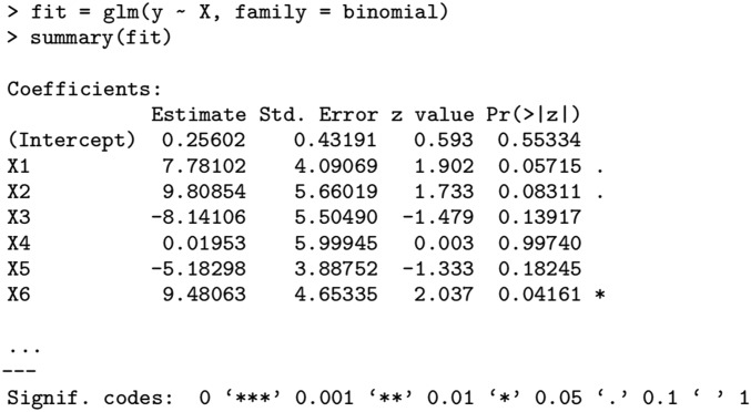
Logistic regression (1, 2) is one of the most frequently used models to estimate the probability of a binary response from the value of multiple features/predictor variables. It is widely used in the social sciences, the finance industry, the medical sciences, and so on. As an example, a typical application of logistic regression may be to predict the risk of developing a given coronary heart disease from a patient’s observed characteristics. Consequently, graduate students in statistics and many fields that involve data analysis learn about logistic regression, perhaps before any other nonlinear multivariate model. In particular, most students know how to interpret the excerpt of the computer output from Fig. 1, which displays regression coefficient estimates, standard errors, and P values for testing the significance of the regression coefficients. In textbooks we learn the following: (i) Fitting a model via maximum likelihood produces estimates that are approximately unbiased. (ii) There are formulas to estimate the accuracy or variability of the maximum-likelihood estimate (MLE) (used in the computer output from Fig. 1).
Fig. 1.
Excerpt from an object of class “glm” obtained by fitting a logistic model in R. The coefficient estimates are obtained by maximum likelihood, and for each variable, R provides an estimate of the SD of as well as a P value for testing whether or not.
These approximations come from asymptotic results. Imagine we have independent observations where is the response variable and the vector of predictor variables. The logistic model posits that the probability of a case conditional on the covariates is given by
where is the standard sigmoidal function. When is fixed and , the MLE obeys
| [1] |
where is the Fisher information matrix evaluated at the true (3). A classical way of understanding Eq. 1 is in the case where the pairs are i.i.d. and the covariates are drawn from a distribution obeying mild conditions so that the MLE exists and is unique. Now the limiting result Eq. 1 justifies the first claim of near unbiasedness. Further, software packages then return standard errors by evaluating the inverse Fisher information matrix at the MLE [this is what R (4) does in Fig. 1]. In turn, these standard errors are then used for the purpose of statistical inference; for instance, they are used to produce P values for testing the significance of regression coefficients, which researchers use in thousands of scientific studies.
Another well-known result in logistic regression is Wilks’ theorem (5), which gives the asymptotic distribution of the likelihood-ratio test (LRT): (iii) Consider the likelihood ratio obtained by dropping variables from the model under study. Then under the null hypothesis that none of the dropped variables belongs to the model, twice the log-likelihood ratio (LLR) converges to a χ2 distribution with degrees of freedom in the limit of large samples. Once more, this approximation is often used in many statistical software packages to obtain P values for testing the significance of individual and/or groups of coefficients.
1. Failures in Moderately Large Dimensions
New technologies now produce extremely large datasets, often with huge numbers of features on each of a comparatively small number of experimental units. However, software packages and practitioners continue to perform calculations as if classical theory applies and, therefore, the main issue is this: Do these approximations hold in high-dimensional settings where is not vanishingly small compared with ?
To address this question, we begin by showing results from an empirical study. Throughout this section, we set and unless otherwise specified, (so that the “dimensionality” is equal to 1/5). We work with a matrix of covariates, which has i.i.d. entries, and different types of regression coefficients scaled in such a way that
This is a crucial point: We want to make sure that the size of the log-odds ratio does not increase with or , so that is not trivially equal to either 0 or 1. Instead, we want to be in a regime where accurate estimates of translate into a precise evaluation of a nontrivial probability. With our scaling , about 95% of the observations will be such that so that .
Unbiasedness?
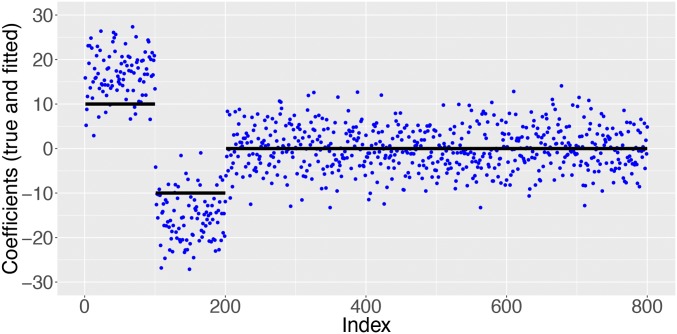
Fig. 2 plots the true and fitted coefficients in the setting where one-quarter of the regression coefficients have a magnitude equal to 10, and the rest are 0. Half of the nonzero coefficients are positive and the other half are negative. A striking feature is that the black curve does not pass through the center of the blue scatter. This disagrees with what we would expect from classical theory. Clearly, the regression estimates are not close to being unbiased. When the true effect size is positive, we see that the MLE tends to overestimate it. Symmetrically, when is negative, the MLE tends to underestimate the effect sizes in the sense that the fitted values are in the same direction but with magnitudes that are too large. In other words, for most indexes so that we are overestimating the magnitudes of the effects.
Fig. 2.
True signal values in black and corresponding ML estimates (blue points). Observe that estimates of effect magnitudes are seriously biased upward.
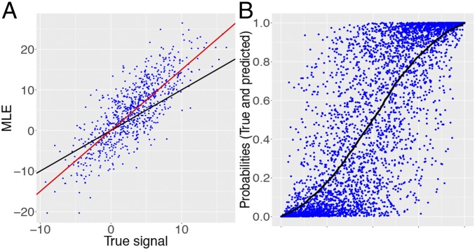
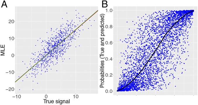
The bias is not specific to this example as the theory we develop in this paper will make clear. Consider a case where the entries of are drawn i.i.d. from (the setup is otherwise unchanged). Fig. 3A shows that the pairs are not distributed around a straight line of slope 1; rather, they are distributed around a line with a larger slope. Our theory predicts that the points should be scattered around a line with slope 1.499 shown in red, as if we could think that .
Fig. 3.
(A) Scatterplot of the pairs for i.i.d. regression coefficients. The black line has slope 1. Again, we see that the MLE seriously overestimates effect magnitudes. The red line has slope predicted by the solution to Eq. 5. We can see that seems centered around . (B) True conditional probability (black curve) and corresponding estimated probabilities (blue points). Observe the dramatic shrinkage of the estimates toward the end points.
This bias is highly problematic for estimating the probability of our binary response. Suppose we are given a vector of covariates and estimate the regression function with
Then because we tend to overestimate the magnitudes of the effects, we will also tend to overestimate or underestimate the probabilities depending on whether is greater or less than a half. This is illustrated in Fig. 3B. Observe that when , many predictions tend to be close to 0, even when is nowhere near 0. A similar behavior is obtained by symmetry; when , we see a shrinkage toward the other end point, namely, 1. Hence, we see a shrinkage toward the extremes and the phenomenon is amplified as the true probability approaches 0 or 1. Expressed differently, the MLE may predict that an outcome is almost certain (i.e., is close to 0 or 1) when, in fact, the outcome is not at all certain. This behavior is misleading.
Accuracy of Classical Standard Errors?
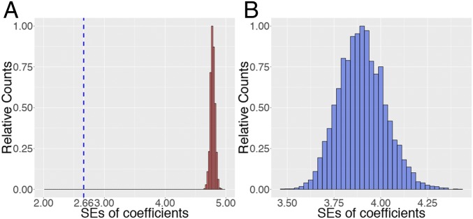
Consider the same matrix as before and regression coefficients now sampled as follows: Half of the s are i.i.d. draws from , and the other half vanish. Fig. 4A shows standard errors computed via Monte Carlo of maximum-likelihood (ML) estimates corresponding to null coordinates. This is obtained by fixing the signal and resampling the response vector and covariate matrix times. Note that for any null coordinate, the classical estimate of SE based on the inverse Fisher information can be explicitly calculated in this setting and turns out to be equal to 2.66 (SI Appendix, section A). Since the SE values evidently concentrate around 4.75, we see that in higher dimensions, the variance of the MLE is likely to be much larger than the classical asymptotic variance. Naturally, using classical results would lead to incorrect P values and confidence statements, a major issue first noted in ref. 6.
Fig. 4.
(A) Distribution of for each variable , in which the SE is estimated from samples. The classical SE value is shown in blue. Classical theory underestimates the variability of the MLE. (B) SE estimates computed from R for a single null (for which ) obtained across replicates resampling the response vector and the covariate matrix.
The variance estimates obtained from statistical software packages are different from the value 2.66 above because they do not take expectation over the covariates and use the MLE in lieu of (plugin estimate) (SI Appendix, section A). Since practitioners often use these estimates, it is useful to describe how they behave. To this end, for each of the samples drawn above, we obtain the R SE estimate for a single MLE coordinate corresponding to a null variable. The histogram is shown in Fig. 4B. The behavior for this specific coordinate is typical of that observed for any other null coordinate, and the maximum value for these standard errors remains below 4.5, significantly below the typical values observed via Monte Carlo simulations in Fig. 4A.
Distribution of the LRT?
By now, the reader should be suspicious that the χ2 approximation for the distribution of the likelihood-ratio test holds in higher dimensions. Indeed, it does not and this actually is not a new observation. In ref. 7, the authors established that for a class of logistic regression models, the LRT converges weakly to a multiple of a χ2 variable in an asymptotic regime in which both and tend to infinity in such a way that . The multiplicative factor is an increasing function of the limiting aspect ratio and exceeds 1 as soon as is positive. This factor can be computed by solving a nonlinear system of two equations in two unknowns given in Eq. 8 below. Furthermore, ref. 7 links the distribution of the LRT with the asymptotic variance of the marginals of the MLE, which turns out to be provably higher than that given by the inverse Fisher information. These findings are of course completely in line with the conclusions from the previous paragraphs. The issue is that the results from ref. 7 assume that ; that is, they apply under the global null where the response does not depend upon the predictors, and it is a priori unclear how the theory would extend beyond this case. Our goal in this paper is to study properties of the MLE and the LRT for high-dimensional logistic regression models under general signal strengths—restricting to the regime where the MLE exists.
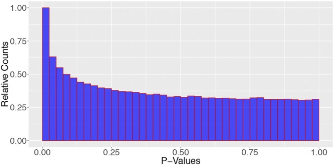
To investigate what happens when we are not under the global null, consider the same setting as in Fig. 4. Fig. 5 shows the distribution of P values for testing a null coefficient based on the χ2 approximation. Not only are the P values far from uniform, but also the enormous mass near 0 is problematic for multiple-testing applications, where one examines P values at very high levels of significance, e.g., near Bonferroni levels. In such applications, one would be bound to make a large number of false discoveries from using P values produced by software packages. To further demonstrate the large inflation near the small P values, we display in Table 1 estimates of the P-value probabilities in bins near 0. The estimates are much higher than what is expected from a uniform distribution. Clearly, the distribution of the LRT is far from a .
Fig. 5.
P values calculated from the approximation to the LLR. Parameters: , with half the coordinates of nonzero, generated i.i.d. from .
Table 1.
P-value probabilities with SEs in parentheses
| Threshold, % | Classical, % |
Here, n=4, 000, p=800, X has i.i.d. Gaussian entries, and half of the entries of β are drawn from (7, 1).
Summary.
We have hopefully made the case that classical results, which software packages continue to rely upon, can be inaccurate in higher dimensions. (i) Estimates seem systematically biased in the sense that effect magnitudes are overestimated. (ii) Estimates are far more variable than classical results. And (iii) inference measures, e.g., P values, are unreliable especially at small values. Given the widespread use of logistic regression in high dimensions, a theory explaining how to adjust inference to make it valid is needed.
2. Our Contribution
We develop a theory for high-dimensional logistic regression models with independent variables that is capable of accurately describing all of the phenomena we have discussed. Taking them one by one, the theory from this paper explicitly characterizes (i) the bias of the MLE, (ii) the variability of the MLE, and (iii) the distribution of the LRT, in an asymptotic regime where the sample size and the number of features grow to infinity in a fixed ratio. Moreover, we shall see that our asymptotic results are extremely accurate in finite-sample settings in which is a fraction of ; e.g., .
A useful feature of this theory is that in our model, all of our results depend on the true coefficients only through the signal strength , where . This immediately suggests that estimating some high-dimensional parameter is not required to adjust inference. We propose in Section 5 a method for estimating and empirically study the quality of inference based on this estimate.
At the mathematical level, our arguments are very involved. Our strategy is to introduce an approximate message-passing algorithm that tracks the MLE in the limit of a large number of features and samples. In truth, a careful mathematical analysis is delicate and we defer the mathematical details to SI Appendix.
3. Prior Work
Asymptotic properties of M estimators in the context of linear regression have been extensively studied in diverging dimensions starting from ref. 8, followed by refs. 9 and 10, in the regime , for some . Later on, the regime where is comparable to became the subject of a series of remarkable works (11–14); these papers concern the distribution of M estimators in linear models. The rigorous results from this literature all assume strongly convex loss functions, a property critically missing in logistic regression. The techniques developed in the work of El Karoui (14) and in ref. 13 play a crucial role in our analysis; the connections are detailed in SI Appendix. While this paper was under review, we also learned about extensions to penalized versions of such strongly convex losses (15). Again, this literature is concerned with linear models only and it is natural to wonder what extensions to generalized linear models might look like; see the comments at the end of the talk (16). More general exponential families were studied in refs. 17 and 18; these works were also in setups subsumed under . Very recently, ref. 19 investigated classical asymptotic normality of the MLE under the global null and regimes in which it may break down as the dimensionality increases.
In parallel, there exists an extensive body of literature on penalized maximum-likelihood estimates/procedures for generalized linear models; see refs. 20 and 21, for example, and the references cited therein. This body of literature often allows to be larger than but relies upon strong sparsity assumptions on the underlying signal. The setting in these works is, therefore, different from ours.
In the low-dimensional setting where the MLE is consistent, finite-sample corrections to the MLE and the LRT have been suggested in a series of works—see, for instance, refs. 22–35. Although these finite-sample approaches aim at correcting the problems described in the preceding sections, that is, the bias of the MLE and nonuniformity of the P values, the corrections are not sufficiently accurate in high dimensions and the methods are often not scalable to high-dimensional data; see SI Appendix, section A for some simulations in this direction. A line of simulation-based results exists to guide practitioners about the sample size required to avoid finite-sample problems (36, 37). The rule of thumb is usually 10 events per variable (EPV) or more but we shall later clearly see that such a rule is not valid when the number of features is large. Ref. 38 contested the previously established 10 EPV rule. To the best of our knowledge, logistic regression in the regime where is comparable to has been quite sparsely studied. This paper follows up on the earlier contribution (7) of the authors, which characterized the LLR distribution in the case where there is no signal (global null). This earlier reference derived the asymptotic distribution of the LLR as a function of the limiting ratio . This former result may be seen as a special case of Theorem 4, which deals with general signal strengths. As is expected, the arguments are now much more complicated than when working under the global null.
4. Main Results
Setting.
We describe the asymptotic properties of the MLE and the LRT in a high-dimensional regime, where and both go to infinity in such a way that . We work with independent observations from a logistic model such that . We assume here that , where is the -dimensional identity matrix. The exact scaling of is not important. As noted before, the important scaling is the signal strength and we assume that the regression coefficients (recall that increases with ) are scaled in such a way that
| [2] |
where is fixed. It is useful to think of the parameter as the signal strength. Another way to express Eq. 2 is to say that .
4.a. When Does the MLE Exist?
The MLE is the minimizer of the negative log-likelihood defined via (observe that the sigmoid is the first derivative of )
| [3] |
A first important remark is that in high dimensions, the MLE does not asymptotically exist if the signal strength exceeds a certain functional of the dimensionality: i.e., . This happens because in such cases, there is a perfect separating hyperplane—separating the cases from the controls if you will—sending the MLE to infinity. It turns out that a companion paper (39) precisely characterizes the region in which the MLE exists.
Theorem 1 (39).
Let be a standard normal variable with density and be an independent continuous random variable with density . With , set
| [4] |
which is a decreasing function of . Then in the setting described above,
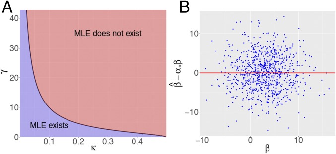
Hence, the curve , or, equivalently, shown in Fig. 6 separates the plane into two regions: One in which the MLE asymptotically exists and one in which it does not. Clearly, we are interested in this paper in the former region (the purple region in Fig. 6A).
Fig. 6.
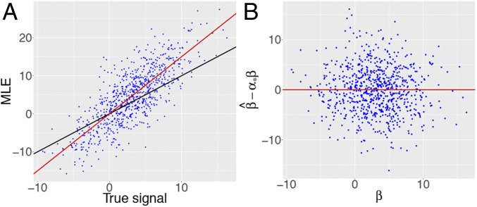
(A) Regions in which the MLE asymptotically exists and is unique and in which it does not. The boundary curve is explicit and given by Eq. 4. (B) In the setting of Fig. 3, scatterplot of the centered MLE vs. the true signal .
4.b. A System of Nonlinear Equations.
As we shall soon see, the asymptotic behavior of both the MLE and the LRT is characterized by a system of equations in three variables ,
| [5] |
where is a bivariate normal variable with mean and covariance
| [6] |
With as in Eq. 3, the proximal mapping operator is defined via
| [7] |
The system of equations in Eq. 5 is parameterized by the pair of dimensionality and signal strength parameters. It turns out that the system admits a unique solution if and only if is in the region where the MLE asymptotically exists!
It is instructive to note that in the case where the signal strength vanishes, , the system of equations in Eq. 5 reduces to the 2-dimensional system
| [8] |
where and . This holds because . It is not surprising that this system is that from ref. 7 since that work considers and, therefore, .
We remark that similar equations have been obtained for M estimators in linear models; see, for instance, ref. 11; SI Appendix, Eqs. S1 and S2; and refs. 13–15.
4.c. The Average Behavior of the MLE.
Our first main result characterizes the “average” behavior of the MLE.
Theorem 2.
Assume the dimensionality and signal strength parameters and are such that (the region where the MLE exists asymptotically and is shown in Fig. 6). Assume the logistic model described above where the empirical distribution of converges weakly to a distribution with finite second moment. Suppose further that the second moment converges in the sense that as , , . Then for any pseudo-Lipschitz function of order 2,† the marginal distributions of the MLE coordinates obey
| [9] |
where , independent of .
Among the many consequences of this result, we give three:
-
•
This result quantifies the exact bias of the MLE in some statistical sense. This can be seen by taking in Eq. 9, which leads to
and says that is centered about . This can be seen from the empirical results from the previous sections as well. When and , the solution to Eq. 5 obeys and Fig. 3A shows that this is the correct centering.
-
•
Second, our result also provides the asymptotic variance of the MLE marginals after they are properly centered. This can be seen by taking , which leads to
As before, this can also be seen from the empirical results from the previous section. When and , the solution to Eq. 5 obeys and this is what we see in Fig. 4.
-
•
Third, our result establishes that upon centering the MLE around , it becomes decorrelated from the signal . This can be seen by taking , which leads to
This can be seen from our earlier empirical results in Fig. 6B. The scatter directly shows the decorrelated structure and the x axis passes right through the center, corroborating our theoretical finding.
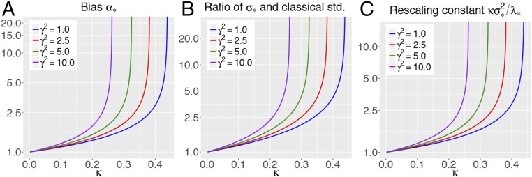
It is of course interesting to study how the bias and the SD depend on the dimensionality and the signal strength . We numerically observe that the larger the dimensionality and/or the larger the signal strength, the larger the bias will be. This dependence is illustrated in Fig. 7A. Further, note that as approaches 0, the bias , indicating that the MLE is asymptotically unbiased if . The same behavior applies to ; that is, increases in either or as shown in Fig. 7B. This plot shows the theoretical prediction divided by the average classical SD obtained from , the inverse of the Fisher information. As approaches 0, the ratio goes to 1, indicating that the classical SD value is valid for ; this is true across all values of . As increases, the ratio deviates increasingly from 1 and we observe higher and higher variance inflation. In summary, the MLE increasingly deviates from what is classically expected as the dimensionality, the signal strength, or both increase.
Fig. 7.
(A) Bias as a function of , for different values of the signal strength . Note the logarithmic scale for the y axis. The curves asymptote at the value of for which the MLE ceases to exist. (B) Ratio of the theoretical SD and the average SD of the coordinates, as obtained from classical theory; i.e., computed using the inverse of the Fisher information. (C) Functional dependence of the rescaling constant on the parameters and .
Theorem 2 is an asymptotic result, and we study how fast the asymptotic kicks in as we increase the sample size . To this end, we set and let half of the coordinates of have constant value 10 and the other half be 0. Note that in this example, as before. Our goal is to empirically determine the parameters and from runs, for each taking values in . Note that there are several ways of determining empirically. For instance, the limit Eq. 9 directly suggests taking the ratio . An alternative is to consider taking the ratio when restricting the summation to nonzero indexes. Empirically, we find there is not much difference between these two choices and choose the latter option, denoting it as . With , the solution to Eq. 5 is equal to . Table 2 shows that is very slightly larger than in finite samples. However, observe that as the sample size increases, approaches , confirming the result from Eq. 9.
Table 2.
Empirical estimates of the centering and SD of the MLE
| Parameter | |||
SEs of these estimates are within parentheses. In this setting, κ=0.1 and γ2 =5. Half of the βjs are equal to 10 and the others to 0.
4.d. The Distribution of the Null MLE Coordinates.
Whereas Theorem 2 describes the average or bulk behavior of the MLE across all of its entries, our next result provides the explicit distribution of whenever , i.e., whenever the th variable is independent from the response .
Theorem 3.
Let be any variable such that . Then in the setting of Theorem 2, the MLE obeys
| [10] |
Further, for any finite subset of null variables , the components of are asymptotically independent.
In words, the null MLE coordinates are asymptotically normal with mean 0 and variance given by the solution to the system Eq. 5. An important remark is this: We have observed that is an increasing function of . Hence, the distribution of a null MLE coordinate depends on the magnitude of the remaining coordinates of the signal: The variance increases as the other coefficient magnitudes increase.
We return to the finite-sample precision of the asymptotic variance . As an empirical estimate, we use averaged over the null coordinates since it is approximately unbiased for . We work in the setting of Table 2 in which , averaging our estimates. The results are given in Table 2; we observe that is very slightly larger than . However, it progressively gets closer to as the sample size increases.
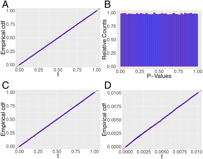
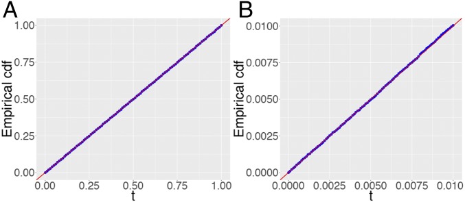
Next, we study the accuracy of the asymptotic convergence results in Eq. 4. In the setting of Table 2, we fit independent logistic regression models and plot the empirical cumulative distribution function of in Fig. 8A for some fixed null coordinate. Observe the perfect agreement with a straight line of slope 1.
Fig. 8.
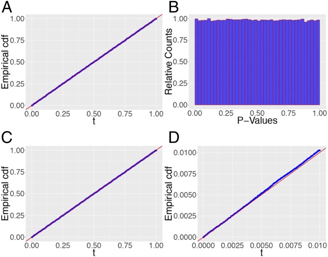
The setting is that from Table 2 with . (A) Empirical cdf of for a null variable (). (B) P values given by the LLR approximation Eq. 11 for this same null variable. (C) Empirical distribution of the P values from B. (D) Same as C but showing accuracy in the lower tail (check the range of the horizontal axis). All these plots are based on 500,000 replicates.
4.e. The Distribution of the LRT.
We finally consider the distribution of the likelihood-ratio statistic for testing .
Theorem 4.
Consider the LLR for testing . In the setting of Theorem 2, twice the LLR is asymptotically distributed as a multiple of a χ2 under the null,
| [11] |
Also, the LLR for testing for any finite converges to the rescaled χ2 under the null.
Theorem 4 explicitly states that the LLR does not follow a distribution as soon as since the multiplicative factor is then larger than 1, as demonstrated in Fig. 7C. In other words, the LLR is stochastically much larger than a , explaining the large spike near 0 in Fig. 5. Also, Fig. 7C suggests that as , the classical result is recovered.‡ We refer the readers to SI Appendix, section G for an empirical comparison of the P values based on Eq. 11 and classical P values in settings with small and moderate .
Theorem 4 extends to arbitrary signal strengths the earlier result from ref. 7, which described the distribution of the LLR under the global null ( for all ). One can quickly verify that when , the multiplicative factor in Eq. 11 is that given in ref. 7, which easily follows from the fact that in this case, Eq. 5 reduces to Eq. 8. Furthermore, if the signal is sparse in the sense that coefficients have nonzero values, then , which immediately implies that the asymptotic distribution for the LLR from ref. 7 still holds in such cases.
To investigate the quality of the accuracy of Eq. 11 in finite samples, we work on the P-value scale. We select a null coefficient and compute P values based on Eq. 11. The histogram for the P values across runs is shown in Fig. 8B and the empirical cumulative distribution function (cdf) in Fig. 8C. In stark contrast to Fig. 4, we observe that the P values are uniform over the bulk of the distribution.
From a multiple-testing perspective, it is essential to understand the accuracy of the rescaled χ2 approximation in the tails of the distribution. We plot the empirical cdf of the P values, zooming in on the tail, in Fig. 8D. We find that the rescaled χ2 approximation works well even in the tails of the distribution. To obtain a more refined idea of the quality of approximation, we zoom in on the smaller bins close to 0 and provide estimates of the P-value probabilities in Table 3 for and . The tail approximation is accurate, modulo a slight deviation in the bin for for the smaller sample size. For , however, this deviation vanishes and we find perfect coverage of the true values. It seems that our approximation is extremely precise even in the tails.
Table 3.
P-value probabilities estimated over replicates with standard errors in parentheses
| Threshold, % | , % | , % |
Here, κ=0.1 and the setting is otherwise the same as in Table 2.
4.f. Other Scalings.
Throughout this section, we worked under the assumption that , which does not depend on , and we explained that this is the only scaling that makes sense to avoid a trivial problem. We set the variables to have variance but this is of course somewhat arbitrary. For example, we could choose them to have variance as in . This means that , where is as before. This gives , where . The conclusions from Theorems 2 and 3 then hold for the model with predictors and regression coefficient sequence . Consequently, by simple rescaling, we can pass the properties of the MLE in this model to those of the MLE in the model with predictors and coefficients . For instance, the SE of is equal to , where is just as in Theorems 2 and 3. On the other hand, the result for the LRT, namely Theorem 4, is scale invariant.
4.g. Non-Gaussian Covariates
Our model assumes that the features are Gaussian. However, we expect that the same results hold under other distributions with the proviso that they have sufficiently light tails. In this section, we empirically study the applicability of our results for certain non-Gaussian features.
In genetic studies, we often wish to understand how a binary response/phenotype depends on single-nucleotide polymorphisms (SNPs), which typically take on values in . When the th SNP is in Hardy–Weinberg equilibrium, the chance of observing 0, 1, and 2 is respectively , , and , where is between 0 and 1. Below we generate independent features with marginal distributions as above for parameters varying in . We then center and normalize each column of the feature matrix to have 0 mean and unit variance. Keeping everything else as in the setting of Fig. 3, we study the bias of the MLE in Fig. 9A. As for Gaussian designs, the MLE seriously overestimates effect magnitudes and our theoretical prediction accurately corrects for the bias. We also see that the bias-adjusted residuals are uncorrelated with the effect sizes , as shown in Fig. 9B.
Fig. 9.
Simulation for a non-Gaussian design. The th feature takes values in with probabilities ; here, and for . Features are then centered and rescaled to have unit variance. The setting is otherwise the same as for Fig. 3. (A) Analogue of Fig. 3A. Red line has slope . (B) Analogue of Fig. 6B. Observe the same behavior as earlier: The theory predicts correctly the bias and the decorrelation between the bias-adjusted residuals and the true effect sizes.
The bulk distribution of a null coordinate suggested by Theorem 3 and the LRT distribution from Theorem 4 are displayed in Fig. 10. Other than the design, the setting is the same as in Fig. 8. The theoretical predictions are once again accurate. Furthermore, upon examining the tails of the P-value distribution, we once more observe a close agreement with our theoretical predictions. All in all, these findings indicate that our theory is expected to apply to a far broader class of features. We conduct additional experiments based on real-data design matrices in SI Appendix, section F.
Fig. 10.
The features are multinomial as in Fig. 9 and the setting is otherwise the same as in Fig. 8. (A) Empirical cdf of for a null variable (). (B) P values given by the LLR approximation Eq. 11 for this same null variable. (C) Empirical distribution of the P values from B. (D) Same as C but displaying accuracy in the extreme. These results are based on replicates.
That said, we caution readers against overinterpreting our results. For linear models, for example, it is known that the distribution of M estimators in high dimensions can be significantly different if the covariates follow a general elliptical distribution, rather than a normal distribution (11, 14).
5. Adjusting Inference by Estimating the Signal Strength
All of our asymptotic results, namely, the average behavior of the MLE, the asymptotic distribution of a null coordinate, and the LLR, depend on the unknown signal strength . In this section, we describe a simple procedure for estimating this single parameter from an idea proposed by Boaz Nadler and Rina Barber after E.J.C. presented the results from this paper at the Mathematisches Forshunginstitut Oberwolfach on March 12, 2018.
5.a. ProbeFrontier: Estimating by Probing the MLE Frontier
We estimate the signal strength by actually using the predictions from our theory, namely, the fact that we have asymptotically characterized in Section 4.a the region where the MLE exists. We know from Theorem 1 that for each , there is a maximum dimensionality at which the MLE ceases to exist. We propose an estimate of and set . Below, we refer to this as the ProbeFrontier method.
Given a data sample , we begin by choosing a fine grid of values . For each , we execute the following procedure:
Subsample.
Sample observations from the data without replacement, rounding to the nearest integer. Ignoring the rounding, the dimensionality of this subsample is .
Check whether MLE exists.
For the subsample, check whether the MLE exists or not. This is done by solving a linear programing feasibility problem; if there exists a vector such that is positive when and negative otherwise, then perfect separation between cases and controls occurs and the MLE does not exist. Conversely, if the linear program is infeasible, then the MLE exists.
Repeat.
Repeat the two previous steps times and compute the proportion of times the MLE does not exist.
We next find , such that is the smallest value in for which . By linear interpolation between and , we obtain for which the proportion of times the MLE does not exist would be 0.5. We set . (Since the “phase-transition” boundary for the existence of the MLE is a smooth function of , as is clear from Fig. 6, choosing a sufficiently fine grid would make the linear interpolation step sufficiently precise.)
5.b. Empirical Performance of Adjusted Inference
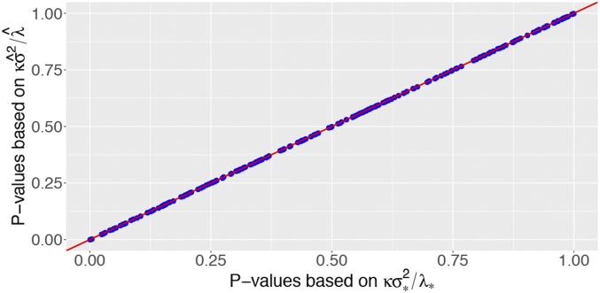
We demonstrate the accuracy of ProbeFrontier via some empirical results. We begin by generating 4,000 i.i.d. observations using the same setup as in Fig. 8 ( and half of the regression coefficients are null). We work with a sequence of points spaced apart by and obtain via the procedure described above, drawing 50 subsamples. Solving the system Eq. 5 using and yields estimates for the theoretical predictions equal to . In turn, this yields an estimate for the multiplicative factor in Eq. 11 equal to . Recall from Section 4 that the theoretical values are and . Next, we compute the LLR statistic for each null and P values from the approximation Eq. 11 in two ways: First, by using the theoretically predicted values, and second, by using our estimates. A scatterplot of these two sets of P values is shown in Fig. 11 (blue). We observe impeccable agreement.
Fig. 11.
Null P values obtained using the approximation plotted against those obtained using . Observe the perfect agreement with the red diagonal.
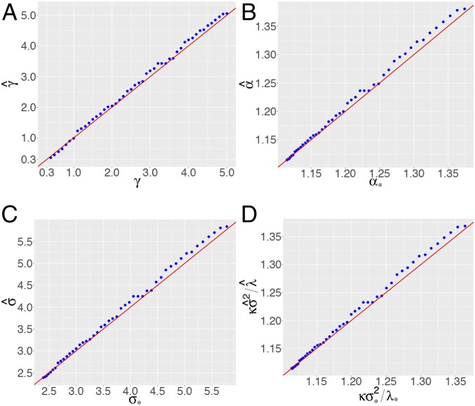
Next, we study the accuracy of across different choices for , ranging from 0.3 to 5. We begin by selecting a fine grid of values and for each, we generate observations with , (so that ), and half the coefficients have a nonvanishing magnitude scaled in such a way that the signal strength is . Fig. 12A displays vs. in blue, and we note that ProbeFrontier works very well. We observe that the blue points fluctuate very mildly above the diagonal for larger values of the signal strength but remain extremely close to the diagonal throughout. This confirms that ProbeFrontier estimates the signal strength with reasonably high precision. Having obtained an accurate estimate for , plugging it into Eq. 5 immediately yields an estimate for the bias , SD, and the rescaling factor in Eq. 11. We study the accuracy of these estimates in Fig. 12 B–D. We observe a similar behavior in all these cases, with the procedure yielding extremely precise estimates for smaller values and reasonably accurate estimates for higher values.
Fig. 12.
(A–D) ProbeFrontier estimates of signal strength (A), bias (B), SD (C), and LRT factor (D) in Eq. 11, plotted against the theoretical values.
Finally, we focus on the estimation accuracy for a particular pair across several replicates. In the setting of Fig. 8, we generate 6,000 samples and obtain estimates of bias (), SD (), and rescaling factor for the LRT (). The averages of these estimates are reported in Table 4. Our estimates always recover the true values up to the first digit. It is instructive to study the precision of the procedure on the P-value scale. To this end, we compute P values from Eq. 11, using the estimated multiplicative factor . The empirical cdf of the P values both in the bulk and in the extreme tails is shown in Fig. 13. We observe perfect agreement with the uniform distribution, establishing the practical applicability of our theory and methods.
Table 4.
Parameter estimates in the setting of Table 2: Averages over 6,000 replicates with SEs within parentheses
| Parameters | True | Estimates |
| 2.2361 | ||
| 1.1678 | ||
| 3.3466 | ||
| 1.166 |
Fig. 13.
(A) Empirical distribution of the P values based on the LLR approximation Eq. 11, obtained using the estimated factor . (B) Same as A, but showing the tail of the empirical cdf. The calculations are based on 500,000 replicates.
5.c. Debiasing the MLE and Its Predictions
We have seen that maximum likelihood produces biased coefficient estimates and predictions. The question is, how precisely can our proposed theory and methods correct this? Recall the example from Fig. 3, where the theoretical prediction for the bias is . For this dataset, ProbeFrontier yields , shown as the green line in Fig. 14A. Clearly, the estimate of bias is extremely precise and coefficient estimates appear nearly unbiased.
Fig. 14.
(A) Scatterplot of the pairs for the dataset from Fig. 3. Here, (red line) and our ProbeFrontier estimate is (green line). The estimate is so close that the green line masks the red. (B) True conditional probabilities (black curve) and corresponding estimated probabilities computed from the debiased MLE (blue points). Observe that the black curve now passes through the center of the blue point cloud. Our predictions are fairly unbiased.
Further, we can also use our estimate of bias to refine the predictions since we can estimate the regression function by . Fig. 14B shows our predictions on the same dataset. In stark contrast to Fig. 3B, the predictions are now centered around the regression function and the massive shrinkage toward the extremes has disappeared. The predictions constructed from the debiased MLE are more accurate and no longer falsely predict almost certain outcomes. Rather, we obtain fairly nontrivial chances of being classified in either of the two response categories—as it should be.
6. Broader Implications and Future Directions
This paper shows that in high dimensions, classical ML theory has limitations; e.g., classical theory predicts that the MLE is approximately unbiased when in reality it overestimates effect magnitudes. Since the purpose of logistic modeling is to estimate the risk of a specific disease given a patient’s observed characteristics, for example, the bias of the MLE is problematic. A consequence of the bias is that the MLE pushes the predicted chance of being sick toward 0 or 1. This, along with the fact that P values computed from classical approximations are misleading in high dimensions, clearly make the case that routinely used statistical tools fail to provide meaningful inferences from both an estimation and a testing perspective.
We have developed a theory which gives the asymptotic distribution of the MLE and the LRT in a model with independent covariates. As seen in Section 4.g, our results likely hold for a broader range of feature distributions (i.e., other than Gaussian) and it would be important to establish this rigorously. Further, we have also shown how to adjust inference by plugging in an estimate of signal strength in our theoretical predictions.
We conclude with a few directions for future work: It would be of interest to develop corresponding results in the case where the predictors are correlated and to extend the results from this paper to other generalized linear models. Further, it is crucial to understand the robustness of our proposed P values to model misspecifications. We provide some preliminary simulations in SI Appendix, section E. Finally, covariates following general elliptical distributions can be challenging, as shown in refs. 11 and 14 in the context of linear models. Hence, caution is in order as to the broader applicability of our theory.
Supplementary Material
Acknowledgments
P.S. was partially supported by a Ric Weiland Graduate Fellowship. E.J.C. was partially supported by the Office of Naval Research under Grant N00014-16-1-2712, by the National Science Foundation via DMS 1712800, by the Math + X Award from the Simons Foundation, and by a generous gift from TwoSigma. P.S. thanks Andrea Montanari and Subhabrata Sen for helpful discussions about approximate message passing. We thank Małgorzata Bogdan, Nikolaos Ignatiadis, Asaf Weinstein, Lucas Janson, Stephen Bates, and Chiara Sabatti for useful comments about an early version of this paper.
Footnotes
The authors declare no conflict of interest.
†A function is said to be pseudo-Lipschitz of order if there exists a constant such that for all , .
‡For the analytically motivated reader, we remark that unlike classical theory, here the asymptotic distribution of the LRT, i.e., Theorem 4, does not follow directly from the asymptotic normality result in Theorem 3. It requires additional probabilistic analysis.
This article contains supporting information online at www.pnas.org/lookup/suppl/doi:10.1073/pnas.1810420116/-/DCSupplemental.
References
- 1.Cox D. R., The regression analysis of binary sequences. J. R. Stat. Soc. Ser. B (Methodol.) 20, 215–232 (1958). [Google Scholar]
- 2.Hosmer D. W., Lemeshow S., Applied Logistic Regression (John Wiley & Sons, 2013), vol. 398. [Google Scholar]
- 3.Van der Vaart A. W., Asymptotic Statistics (Cambridge University Press; ), vol. 3. [Google Scholar]
- 4.R Core Team , R: A Language and Environment for Statistical Computing (R Foundation for Statistical Computing, Vienna, Austria, 2018). [Google Scholar]
- 5.Wilks S. S., The large-sample distribution of the likelihood ratio for testing composite hypotheses. Ann. Math. Stat. 9, 60–62 (1938). [Google Scholar]
- 6.Candes E., Fan Y., Janson L., Lv J., Panning for gold: ‘Model-x’ knockoffs for high dimensional controlled variable selection. J. R. Stat. Soc. Ser. B (Stat. Methodol.) 80, 551–577 (2018). [Google Scholar]
- 7.Sur P., Chen Y., Candès E. J., The likelihood ratio test in high-dimensional logistic regression is asymptotically a rescaled chi-square. Probab. Theory Relat. Fields, 10.1007/s00440-018-00896-9 (23 January 2019). [DOI] [Google Scholar]
- 8.Huber P. J., Robust regression: Asymptotics, conjectures and Monte Carlo. Ann. Stat. 1, 799–821 (1973). [Google Scholar]
- 9.Portnoy S., Asymptotic behavior of M-estimators of regression parameters when is large. I. Consistency. Ann. Stat. 12, 1298–1309 (1984) . [Google Scholar]
- 10.Portnoy S., Asymptotic behavior of M-estimators of regression parameters when is large; II. Normal approximation. Ann. Stat. 13, 1403–1417 (1985). [Google Scholar]
- 11.El Karoui N., Bean D., Bickel P. J., Lim C., Yu B., On robust regression with high-dimensional predictors. Proc. Natl. Acad. Sci. U.S.A 110, 14557–14562(2013). [DOI] [PMC free article] [PubMed] [Google Scholar]
- 12.Bean D., Bickel P. J., El Karoui N., Yu B., Optimal m-estimation in high-dimensional regression. Proc. Natl. Acad. Sci. U.S.A. 110, 14563–14568 (2013). [DOI] [PMC free article] [PubMed] [Google Scholar]
- 13.Donoho D., Montanari A., High dimensional robust M-estimation: Asymptotic variance via approximate message passing. Probab. Theory Relat. Fields 166, 935–969 (2013). [Google Scholar]
- 14.El Karoui N., On the impact of predictor geometry on the performance on high-dimensional ridge-regularized generalized robust regression estimators. Probab. Theory Relat. Fields 170, 95–175 (2017). [Google Scholar]
- 15.Bradic J., Robustness in sparse high-dimensional linear models: Relative efficiency and robust approximate message passing. Electron. J. Stat. 10, 3894–3944(2016). [Google Scholar]
- 16.El Karoui N., Random matrices and high-dimensional M-estimation: Applications to robust regression, penalized robust regression and GLMs. https://video.seas.harvard.edu/media/14_03_31+Noureddine+El+Karoui–AM.mp4/1_e5szurf0/13151391 (31 March 2014).
- 17.Portnoy S., Asymptotic behavior of likelihood methods for exponential families when the number of parameters tends to infinity. Ann. Stat. 16, 356–366 (1988). [Google Scholar]
- 18.He X., Shao Q. M., On parameters of increasing dimensions. J. Multivariate Anal. 73, 120–135 (2000). [Google Scholar]
- 19.Fan Y., Demirkaya E., Lv J., Nonuniformity of p-values can occur early in diverging dimensions. arXiv:1705.03604 (10 May 2017). [PMC free article] [PubMed]
- 20.Bunea F., Honest variable selection in linear and logistic regression models via l1 and l1+l2 penalization. Electron J. Stat. 2, 1153–1194 (2008). [Google Scholar]
- 21.Van de Geer S., Bühlmann P., Ritov Y., Dezeure R., On asymptotically optimal confidence regions and tests for high-dimensional models. Ann. Stat. 42, 1166–1202 (2014). [Google Scholar]
- 22.Firth D., Bias reduction of maximum likelihood estimates. Biometrika 80, 27–38 (1993). [Google Scholar]
- 23.Anderson J., Richardson S., Logistic discrimination and bias correction in maximum likelihood estimation. Technometrics 21, 71–78 (1979). [Google Scholar]
- 24.McLachlan G., A note on bias correction in maximum likelihood estimation with logistic discrimination. Technometrics 22, 621–627 (1980). [Google Scholar]
- 25.Schaefer R. L., Bias correction in maximum likelihood logistic regression. Stat. Med. 2, 71–78 (1983). [DOI] [PubMed] [Google Scholar]
- 26.Copas J. B., Binary regression models for contaminated data. J. R. Stat. Soc. Ser. B (Methodol.) 50, 225–253 (1988). [Google Scholar]
- 27.Cordeiro G. M., McCullagh P., Bias correction in generalized linear models. J. R. Stat. Soc. Ser. B (Methodol.) 53, 629–643 (1991). [Google Scholar]
- 28.Bull S., Hauck W., Greenwood C., Two-step jackknife bias reduction for logistic regression MLEs. Commun. Stat. Simul. Comput. 23, 59–88 (1994). [Google Scholar]
- 29.Jennings D. E., Judging inference adequacy in logistic regression. J. Am. Stat. Assoc. 81, 471–476 (1986). [Google Scholar]
- 30.Bartlett M. S., Properties of sufficiency and statistical tests. Proc. R. Soc. Lond. Ser. A Math. Phys. Sci. 160, 268–282 (1937). [Google Scholar]
- 31.Box G., A general distribution theory for a class of likelihood criteria. Biometrika 36, 317–346 (1949). [PubMed] [Google Scholar]
- 32.Lawley D., A general method for approximating to the distribution of likelihood ratio criteria. Biometrika 43, 295–303 (1956). [Google Scholar]
- 33.Cordeiro G. M., Improved likelihood ratio statistics for generalized linear models. J. R. Stat. Soc. Ser. B (Methodol.) 45, 404–413 (1983). [Google Scholar]
- 34.Bickel P. J., Ghosh J., A decomposition for the likelihood ratio statistic and the Bartlett correction–A Bayesian argument. Ann. Stat. 18, 1070–1090 (1990). [Google Scholar]
- 35.Moulton L. H, Weissfeld L. A., Laurent R. T. S., Bartlett correction factors in logistic regression models. Comput. Stat. Data Anal. 15, 1–11 (1993). [Google Scholar]
- 36.Peduzzi P., Concato J., Kemper E., Holford T. R., Feinstein A. R., A simulation study of the number of events per variable in logistic regression analysis. J. Clin. Epidemiol. 49, 1373–1379 (1996). [DOI] [PubMed] [Google Scholar]
- 37.Vittinghoff E., McCulloch C. E., Relaxing the rule of ten events per variable in logistic and Cox regression. Am. J. Epidemiol. 165, 710–718 (2007). [DOI] [PubMed] [Google Scholar]
- 38.Courvoisier D. S., Combescure C, Agoritsas T., Gayet-Ageron A., Perneger T. V., Performance of logistic regression modeling: Beyond the number of events per variable, the role of data structure. J. Clin. Epidemiol. 64, 993–1000 (2011). [DOI] [PubMed] [Google Scholar]
- 39.Candès E. J., Sur P., The phase transition for the existence of the maximum likelihood estimate in high-dimensional logistic regression. arXiv:1804.09753 (25 April 2018). [Google Scholar]
Associated Data
This section collects any data citations, data availability statements, or supplementary materials included in this article.


