Neural Representation of Object Approach in a Decision-Making Motor Circuit

Abstract

Although behavior is ultimately guided by decision-making neurons and their associated networks, the mechanisms underlying neural decision-making in a behaviorally relevant context remain mostly elusive. To address this question, we analyzed goldfish escapes in response to distinct visual looming stimuli with high-speed video and compared them with electrophysiological responses of the Mauthner cell (M-cell), the threshold detector that initiates such behaviors. These looming stimuli evoke powerful and fast body-bend (C-start) escapes with response probabilities between 0.7 and 0.91 and mean latencies ranging from 142 to 716 ms. Chronic recordings showed that these C-starts are correlated with M-cell activity. Analysis of response latency as a function of the different optical parameters characterizing the stimuli suggests response threshold is closely correlated to a dynamically scaled function of angular retinal image size, θ(t), specifically κ(t) = θ(t − δ × e^{−βθ(t − δ)}, where the exponential term progressively reduces the weight of θ(t). Intracellular recordings show that looming stimuli typically evoked bursts of graded EPSPs with peak amplitudes up to 9 mV in the M-cell. The proposed scaling function κ(t) predicts the slope of the depolarizing envelope of these EPSPs and the timing of the largest peak. An analysis of the firing rate of presynaptic inhibitory interneurons suggests the timing of the EPSP peak is shaped by an interaction of excitatory and inhibitory inputs to the M-cell and corresponds to the temporal window in which the probabilistic decision of whether or not to escape is reached.

Introduction

Any organism has to decide whether an approaching object poses a potential danger and when to initiate a properly timed avoidance response, namely, one that is fast but does not occur too soon, which might otherwise allow the predator to correct its strike trajectory (Dill, 1974). Neural computation of an appropriate timing often involves perception of visual motion. For example, an object on collision course creates an image that symmetrically expands across the retina with distinct spatial and temporal characteristics and is perceived as a looming threat (Gibson, 1979). Behavioral experiments show that many animals respond aversely at distinct values of angular image size (Schiff, 1965; Holmqvist and Srinivasan, 1991; Robertson and Johnson, 1993; Yamamoto et al., 2003) or its expansion velocity (Dill, 1974).

Electrophysiological recordings in insects and birds established that different classes of looming neurons, which presumably receive input from arrays of local movement detectors, encode different aspects of the growing retinal image. They include the time to collision (TTC), the angular retinal image size, its expansion velocity, and a nonlinear transformation of size and velocity (Hatsopoulos et al., 1995; Rind and Simmons, 1992, 1996; Sun and Frost, 1998; Gabbiani et al., 2001, 2002; Wicklein and Strausfeld, 2000). The latter combination gives added weight to image expansion velocity initially and deemphasizes it with time (Laurent and Gabbiani, 1998). However, the mechanisms underlying the transformation of encoded sensory information into a motor command (i.e., the neural correlates of information decoding) remain mostly elusive. Teleost escape behavior is a good model for studying these issues because the decision-making network is not broadly distributed. Rather, the final decision is made at the level of a single identifiable reticulospinal neuron that is accessible for intracellular recordings in vivo, the Mauthner cell (M-cell) (Korn and Faber, 2005). Furthermore, it is the prototype of an integrate-and-fire neuron, because its soma-dendritic membrane is inexcitable (Zottoli and Faber, 2000). The paired M-cells receive mechanosensory and visual inputs onto their lateral and ventral dendrites, respectively (Faber and Korn, 1978; Zottoli et al., 1987, 1995; Canfield, 2003). The tectal output also projects to midbrain interneurons that mediate a powerful feedforward inhibition of the M-cell (Zottoli et al., 1987). A single action potential in one M-cell is sufficient to activate contralateral motor execution networks for the initiation of a powerful and fast body-bend (C-start) away from the side of the excited cell. Thus, an escape behavior is initiated if the integration of excitatory and inhibitory inputs exceeds the threshold for spike generation in a single M-cell.

The rationale of this study was to quantify escapes in response to a variety of defined visual looming stimuli, to predict the stimulus-related function that determines the escape likelihood and its timing. We then asked whether that function predicts distinct characteristics of the PSPs recorded intracellularly in the M-cell of restrained goldfish, as well as how it is implemented at the cellular level.

Materials and Methods

Behavior.

Behavioral experiments were performed with individual goldfish (N = 63), 10–13 cm in length, in a temperature-controlled (18°C) circular tank (diameter, 76 cm) resting on an anti-vibration table and surrounded by opaque covers [for details of the setup and animal maintenance, see Preuss and Faber (2003)]. A magnified ventral view of the animals was recorded with two high-speed video cameras (1000 frames/s) with one camera recording a 28 × 21.5 cm area in the center of the tank at high magnification, for high-resolution kinematics including the timing of response onset, and the second one recording behavior in the entire tank. A third standard video camera recorded a lateral view for depth measurement. Looming stimuli consisted of computer-generated series of black (70–80 lux) disk images of increasing size successively projected with a liquid crystal display (LCD) projector (1024 × 768 pixels, 60 Hz refresh rate) onto a translucent white (300–320 lux) screen fixed 16 cm above the fish (see Fig. 1). The water height in the tank was 6 cm, which ensures a relatively defined distance between the fish and the screen by restricting locomotion to two dimensions, with the uncertainty in the height being ∼1 cm. The angular retinal image size of the looming object as seen by the fish was approximated for a 16 cm vertical distance between the head and the projection screen (see Fig. 2A). The animals were free to move in the tank; however, only responses in the apparent collision trajectory of the stimulus were used for data analysis.

Figure 1.

Visual-evoked escapes in goldfish. A, Behavioral setup and stimulus presentation. Left and top right, Projecting the image of an expanding disk onto a screen above the animal triggers a short-latency body bend (top right). Bottom right, Chronic recordings of brainstem activity show a single Mauthner axon spike (*) preceding a visual evoked C-start. Later impulses are attributed to firing of other reticulospinal neurons. The bottom trace indicates onset and offset of the looming stimulus (Stim.). The apparent collision time (c.t.) is indicated by an arrowhead. B, Stimulus characterization. Plotted is the time course of the projected disk size (diameter) for eight different stimuli used in the behavior and physiology experiments. Characteristics of three additional control stimuli are described in Results. C, Mean response latencies (open bars) and their relationship to TTC (dark bars) for seven different stimuli that differ in size and/or approach velocity (± SEM; n = number of responses in N = number of animals). D, Stimulus-specific cumulative response probabilities plotted against response latencies normalized with respect to stimulus duration. The numbers distinguish individual stimuli. Stimulus notations and sample sizes apply to Figures 23–4.

Figure 2.

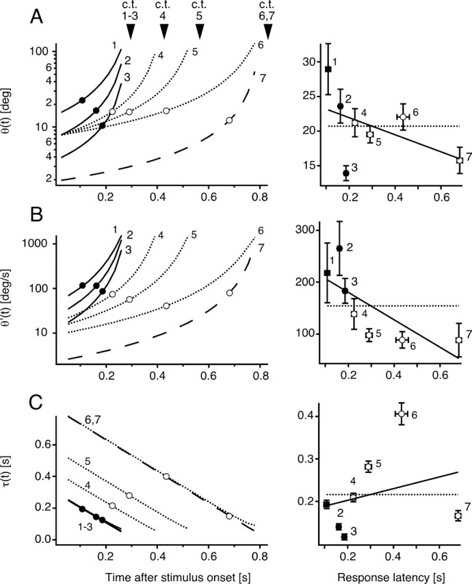
Elementary optical parameters of looming stimuli at response onset. Left, Time course of θ(t) (A), θ′(t) (B), and τ(t) (C) for seven different looming stimuli with corresponding mean escape latencies for stimuli 1–3 (black dots) and stimuli 4–7 (open circles). The apparent collision time (c.t.) for each stimulus is indicated by an arrowhead. To account for 25 ms central processing time (Canfield, 2003) and 10 ms motor output delay (Preuss and Faber, 2003), latencies were adjusted by 35 ms. Note that τ(t) is independent of object size and thus similar for stimuli 1–3. The right panels are plots of the mean escape latencies (±SEM, horizontal error bars) versus the mean threshold values at response onset (±SEM, vertical error bars) for stimuli 1–7 (±SEM). The solid black lines indicate the best linear fits of threshold values, whereas dotted lines are the best horizontal linear fits of the data. Statistical comparison (GEE method and ANOVA) of the threshold values showed significant differences for θ(t), θ′(t), and τ(t) (see Results).

Stimulus design.

The eight looming stimuli that were used differed in either their projected absolute size or apparent approach velocity (see Fig. 1B,C). Subsets of the stimuli had either the same approach velocity of 60 cm/s but different initial absolute sizes (see Fig. 1B, stimuli 1, 2, 3, and 8) or the same absolute size but different approach velocities (see Fig. 1B, stimuli 2, 4, 5, and 6 or stimuli 7 and 8). However, each stimulus has a distinct time course with respect to its projected size. Object size was also quantified as the angular retinal image size θ(t), subtended at the position of the eyes, namely as 2 × tan⁻¹ (d/2 s), where d is the diameter of the projected disk on the screen and s is the distance from the screen to the eye (see Fig. 1A,B). The distance s was nearly constant, given the low water height and the restriction of the data analysis to fish in the center of the experimental tank (see Fig. 1A). The initial angular image size, θ(t = 0), ranged from 2 to 16°, whereas approach velocities, V, varied from 20 to 60 cm/s. Of the eight looming stimuli, only one was essentially subthreshold (stimulus 8). Responses to that stimulus were not further analyzed. It had small initial and final projected sizes, and the former was not the limiting factor, because stimulus 7, which had the same initial size but a slower approach velocity, was quite effective. The different stimuli were presented typically twice per session and in random order and time intervals ranging between 1 and 10 min. Latency, probability, and kinematics of evoked responses were analyzed at 1 ms time resolution as described previously (Preuss and Faber, 2003). Response latency was defined as the interval from stimulus onset to the first detectable movement of the head after the stimulus and was measured manually in successive video images. Stimulus onset was determined from the video image. Peak angular velocity and peak acceleration of the initial C-bend were calculated from smoothed (10 factor Binomial; Igor Pro; WaveMetrics, Lake Oswego, OR) x, y position data of the fish head (rostral end) and the body (center of mass) in successive video frames using NIH Image.

Chronic recordings in behaving fish.

To verify that visual evoked C-starts are associated with an action potential in one of the M-cells, we performed a series of behavioral experiments (N = 3) with chronically implanted monopolar electrodes following established methods (Zottoli, 1977), with the exception that we recorded from the caudal brainstem, where the two M-axons are within 50 μm of the dorsal surface. This allows us to visually guide the placement of the recording electrode and to monitor the activity of both M-axons during evoked escapes.

Data analysis of behavioral experiments.

Escape latency data for all seven effective looming stimuli were used to test whether any of the two elementary critical optical parameters θ(t) and θ′(t), or a combination of the two, specifically, τ, τ(t) = θ(t)/θ′(t); η, η(t) = θ′(t − δ) × e^{−αθ(t − δ)} (Hatsopoulos et al., 1995); κ, κ(t) = θ(t − δ) × e^{−βθ(t − δ)}; and ω, ω(t) = θ′(t − δ) × e^{−ϵθ′(t − δ)}, best fit the notion of a common threshold value. That is, if a given function determines the timing of response onset, it should have the same value for all effective stimuli, and we call that its threshold value. According to Hatsopoulos et al. (1995), δ represents a time delay in the system, as a result of processing time. However, in our behavioral, studies it also includes the motor output delay. We assumed δ was equal to 35 ms, based on a minimal 25 ms delay in central processing of visual information (Zottoli et al., 1987; Canfield, 2003) and an additional 10 ms delay from M-cell firing to response onset (Zottoli, 1977; Preuss and Faber, 2003).

For θ(t), θ′(t), and τ(t), mean values at threshold were calculated for the adjusted response onset time (latency minus 35 ms) for all escapes (n = 305) from 63 fish and compared statistically using a single-factor ANOVA and the generalized estimating equation (GEE) method (Liang and Zeger, 1986) with the null hypothesis being there are no differences among the stimuli. For the κ(t), ω(t), and η(t) functions, the corresponding coefficients in the exponential terms β, ϵ, and α were optimized for each of 60 fish that responded to at least three different stimuli in the center of the tank, by systematically testing a wide range of values for the coefficients, calculating the related function and then minimizing the variance between the calculated mean values of that function at threshold (i.e., at escape onset minus 35 ms sensory and motor processing time). Mean values of β, ϵ, and α were then used to calculate the threshold values for the corresponding functions at escape onset for all individual responses and compared using ANOVA and GEE. These values were also compared with those obtained with a modification of the method proposed by Sun and Frost (1998) and Gabbiani et al. (1999), in which values of β, ϵ, and α can be calculated from the slopes of plots of the behavioral latency, expressed in terms of TTC, versus d/V or (d/V)^1/2, where d is equal to 2 l in the notation used by Gabbiani et al. (1999).

Electrophysiology.

Intracellular responses of the M-cell to visual stimuli were studied in vivo using standard electrophysiological recording and data acquisition techniques (Faber and Korn, 1978). Goldfish were anesthetized initially in ice water and during the experiments by using local anesthetics (20% benzocaine) applied to the wound sites. The fish head was stabilized in the recording chamber by four pins, two on each side, further immobilized with intracellular injections of d-tubocurarine (1–3 μg/g body weight), and respirated through the mouth with aerated saline. The surgical and recording procedures were similar to those described previously (Faber and Korn, 1978). The goal in the electrophysiological experiments was to match the stimulus conditions of the behavioral experiments as close as possible. Thus, the recording chamber was mounted inside a larger opaque tank (height, 30 cm; width, 41 cm; depth, 29 cm) filled with saline to 1 cm above the fish head. Saline maintains viability of the exposed brain and the eyes. The fish was fixed in an upright position with a projection screen 16 cm above the fish head. The trajectory of the approaching object was aligned to the center of the eyes. The visual stimuli used were the same as in the behavioral experiments.

Current-clamp and single-electrode voltage-clamp (SEVC) recordings were obtained from the M-cell ventral dendrite or cell body with electrodes (5–10 MΩ) filled with 5 m K-acetate. IPSCs evoked by visual looming stimuli were measured with the M-cell clamped at its resting potential and during a depolarizing voltage step that began and ended just before and after a given stimulus using established recording and analyzing methods (Faber and Korn, 1988). Data were recorded on-line with a Macintosh G4 (Apple Computers, Cupertino, CA), using acquisition software developed in the laboratory (sampling rate, 10–30 μs) and analyzed with the same software and with Igor Pro. The output of a photodiode in the light path of the LCD projector provided information on the onset and offset of the looming stimulus and was recorded together with the electrophysiological data. All experiments were performed in accordance with relevant guidelines and regulations of the Animal Institute Committee of Albert Einstein College of Medicine.

Data analysis of electrophysiology experiments.

In the electrophysiology experiments, we used exclusively test stimuli 1–6, as well as the control stimuli described in Results. Two parameters were calculated for comparison with the behavioral data, the slope of the compound PSP and the peak time. Slopes of the compound PSPs were calculated using an algorithm that first fits the response with a 25th order polynomial, then defines a baseline as the variance, σ², of the first derivative, from a 50 ms period before stimulus onset. Then, it detects PSP onset and peak from that first derivative. PSP onset was taken as the first point with a slope greater than σ. PSP slope was the mean slope between the onset and peak of a response. Unless otherwise stated, n equals the number of responses and N equals the number of animals used.

Statistical tests.

ANOVA is a commonly used method to compare means among groups and requires the assumption that the observations are independent and normally distributed with constant variance. However, in our experiment, the multiple measurements from the same fish are likely to be correlated, thereby violating the independence assumption. The GEE method is a common approach for analyzing repeated measures data and is an extension of generalized linear models (McCullagh and Nelder, 1989). The method allows for regression modeling of repeated-measures data, specifying only the mean and variance of the outcome variables and requires no assumptions regarding the distribution of the outcome variables. Furthermore, the correlation among measurements from the same fish is taken into account in the estimation of the regression coefficients and their SEs. The GEE method yields consistent estimates of the regression coefficients even if the assumed correlation structure is incorrect. Thus, the GEE analysis is the preferred model here. The GEE analysis produces either the same or more conservative p values when compared with those of a single-factor ANOVA. Therefore, we only report the GEE values here.

Results

Visual-evoked C-starts

We examined 315 escapes evoked in 409 trials with 63 goldfish in response to a visual looming stimulus consisting of a small black dot that is projected on a screen above the animal and rapidly expands in size (Fig. 1A). The evoked behavior was characterized by a brisk initial C-shaped bend of the animal head and tail (Fig. 1A) followed by a return flip associated with forward propulsion [stages 1 and 2 in Foreman and Eaton (1993)]. High-speed kinematic measurements of the initial C-bend showed a mean peak angular velocity of 3515 °/s ± 309 SEM and a mean peak angular acceleration of 452 °/s²± 55 SEM (N = 5; n = 57). These values are comparable with those reported previously for C-starts evoked by short sound clicks (Preuss and Faber, 2003). Fish in the direct collision trajectory of the stimulus showed no clear directional preference for left or right turns (58 vs 42%, respectively).

Previous studies with acoustic stimuli established that a single action potential in one M-cell activates contralateral spinal motor execution networks, causing a fast body-bend starting 7.5 ms after M-cell firing (Zottoli, 1977; Eaton et al., 1981). Chronic extracellular recordings from the M-axons in the brainstem in free-behaving goldfish, shown in Figure 1A, demonstrate that this is also the case for escapes evoked by visual looming stimuli; the mean time from the M-spike to movement onset was 7.85 ± 0.83 ms (SEM; n = 9). The M-cell fired before every visual evoked response (19% response probability in 47 trials, three animals, alternating between stimulus 1 and 6) and its action potential consistently preceded the neural activity of other reticulospinal axons (Fig. 1A, bottom right). Correspondingly, every M-cell spike was associated with a behavioral response.

We next asked how the probability and timing of an escape varied with stimulus parameters. Overall, response probability ranged from 0.7 to 0.91, as shown by the cumulative probability plots in Figure 1D, with the relatively smaller and faster stimuli being the least effective (e.g., stimuli 2 and 3). These are also some of the shortest-lasting stimuli. The failure to trigger behavioral responses in some trials is not caused by variability of the position of the fish with respect to the stimulus, because the analysis is restricted to fish in the center of the tank (i.e., in the object's simulated approach path). In fact, when the analysis was expanded to include trials in which the fish was off center (n = 254), the response probabilities were smaller, ranging from 0.55 to 0.85, but the mean latencies were not significantly different (p = 0.123). These response probabilities are significantly higher than that found with the combined behavioral and chronic electrophysiological experiments (0.19), presumably because of the effect of fish handling and electrode implantation in the latter series.

The seven effective looming stimuli (see Material and Methods) elicited escapes with significantly different mean latencies (p < 0.0001), which depended on initial angular image size and approach speed; larger and faster objects produce shorter escape latencies (Fig. 1C). In all cases, however, the mean escape latency was appreciably shorter than stimulus duration (40–80%) (Fig. 1D). When these latencies are converted to the corresponding time to collision, they range from 99 ms, for stimulus 3, to 396 ms, for stimulus 6. In general, faster or smaller stimuli evoked behavioral responses at the shorter times to collision (Fig. 1C, left panels). The mean latencies (142–716 ms) of responses evoked by the different looming stimuli are in a range that is one to two orders of magnitude longer than those associated with escapes evoked by short (5 ms) sound clicks (Preuss and Faber, 2003). This difference likely reflects the more complex information processing in the polysynaptic retinal and tectal pathways compared with the disynaptic connection from the inner ear to the M-cell. Essentially no responses were evoked by large size black disks that decreased in size (1 in 29 trials) or by large black disks of fixed size that suddenly appeared on the screen (0 in 57 trials). In another set of control experiments the overall luminance change was minimized by using a looming stimulus consisting of a black and white checkerboard pattern disk that emerged from a blue background (Wang et al., 1993). These experiments showed no significant differences in escape probability and latency with those that used the solid black disk. Together, these results suggest that the elicited responses were looming specific, in that fish responded vigorously to a simulated approaching object but not to the sudden appearance of a static object or to a sudden change in overall luminance).

Characterization of critical optical stimulus parameters

The looming stimuli we used have had distinct time courses with respect to the different optical parameters that theoretically can be extracted from the retinal motion pattern that is produced by an object approaching on a collision course. This diverse set of stimuli allows us to ask which, if any, of the optical parameters is correlated with the onset of the behavior. Figure 2 illustrates the angular retinal image size of the simulated object over time, θ(t), and its expansion velocity, θ′(t). θ(t) and θ′(t) grow in nonlinear, near-to-exponential manner, with the largest increase just before impact (Fig. 2A,B). A third parameter commonly associated with detection of looming stimuli of constant approach velocity is the time to collision, τ(t) = θ(t)/θ′(t) (Gibson, 1961). Indeed, there is evidence that this parameter is encoded in the pigeon visual system (Wang and Frost, 1992; Sun and Frost, 1998) and in humans (Regan and Vincent, 1995; Regan, 2002) (but see Tresilian, 1999). For small objects, τ declines linearly as a function of approach speed and is independent of object size (Fig. 2C) (Gibson, 1961). If one of these parameters determines a certain threshold for triggering the behavior, its value should be the same at a fixed time before the response occurs for all stimuli.

Plots of the values of θ(t), θ′(t), and τ(t) at mean response latency minus 35 ms for the seven effective looming stimuli would seem to suggest that behavioral threshold is more likely to be correlated with a constant value of θ(t) or θ′(t) rather than τ(t) (Fig. 2A–C, left). However, statistical analyses indicate that none of these three functions actually fulfils the requirement of a constant value at the time of response onset. For each parameter, the means for the seven stimuli are significantly different (p = 0.022, p = 0.019, and p < 0.0001 for θ(t), θ′(t), and τ(t), respectively). This lack of agreement is also illustrated by the plots in Figure 2A–C of the mean parameter values, calculated from individual trials, versus the mean latencies. Thus, neither one of the parameters, θ(t) and θ′(t) or τ(t), seemed to fit the criterion of a fixed value at response onset for all stimuli.

The behavioral data provide indications of the expected form of the optical functions that determine the escape threshold. For example, most escapes occur before θ(t) or θ′(t) peak (Fig. 2A,B), as indicated by the observation that the steepest slopes of the cumulative escape probability plots are between 40 and 80% of stimulus duration (Fig. 1D). Furthermore, the cumulative escape probability is as low as 70% for some of the stimuli, consistent with the notion that the behavior occurs before the object approach has finished. This property is not attributable to an input saturation of the retinal image before stimulus expansion ended because: (1) whereas the mean subtended angular size of an approaching object at response onset was only 21°, the visual field of the goldfish eye is ∼190° (Trevarthen, 1968) and looming-sensitive neurons in zebrafish have receptive field sizes of up to 30° (Sajovic and Levinthal, 1983), and (2) in a control experiment, a looming stimulus with an exceptionally large initial angular size of 22° evoked responses in 91% of the trials (24 responses in eight animals), with a mean latency of 150 ms (mean angular size at response onset, ∼48°). That latency implies a looming-specific response.

Together, the behavioral results suggest that the stimulus becomes less effective in eliciting an escape before it reaches its maximum angular size. This prediction would be consistent with electrophysiological studies in zebrafish, pigeons, and locusts demonstrating that the firing rate of certain classes of looming-sensitive neurons reaches a distinct peak and then declines well before the stimulus peaks (Sajovic and Levinthal, 1983; Hatsopoulos et al., 1995; Sun and Frost, 1998; Gabbiani et al., 1999, 2001).

It was postulated for these other systems that the instantaneous firing rate of individual neurons could be described by a function, η(t), which peaks before stimulus offset. This function essentially requires multiplication of two different optical parameters, namely an input that is proportional to image expansion velocity, θ′(t), and is presumably excitatory, and a second signal that is a function of retinal image size and is presumably inhibitory (Hatsopoulos et al., 1995; Gabbiani et al., 2002, 2005) (but see Rind and Santer, 2004). Specifically, η(t) = θ′(t − δ) × e^{−αθ(t −δ)} (Hatsopoulos et al., 1995). We tested, in addition to η(t), two additional functions that also peak before stimulus offset but are determined by the multiplication of excitatory and inhibitory inputs that depend only on angular image size alone or image expansion velocity alone. These functions are κ, κ(t) = θ(t − δ) × e^{−βθ(t − δ)} and ω, ω(t) = θ′(t − δ) × e^{−ϵθ′(t − δ)} (Fig. 3, left). In all three cases, the exponential term, such as e^{−βθ(t − δ)}, is a dynamic scaling factor that has the effect of progressively reducing the weight of the growing optical parameter, θ(t) or θ′(t). That is, the scaling factor underlies the early peak and decline of these functions. Each of these scaling functions was optimized by first identifying the mean value for the coefficients, α, β, and ϵ, in the exponential terms for the functions η(t), κ(t), and ω(t) (Table 1) that minimized the variance in that function at response onset (see Material and Methods). These calculations assumed the constant behavioral delay, δ, of 35 ms. We then calculated the individual values for η(t), κ(t), and ω(t) at the adjusted escape onset time for a total of 305 responses in 63 fish and compared them statistically with the null hypothesis that they are the same for all seven stimuli (see Material and Methods).

Figure 3.

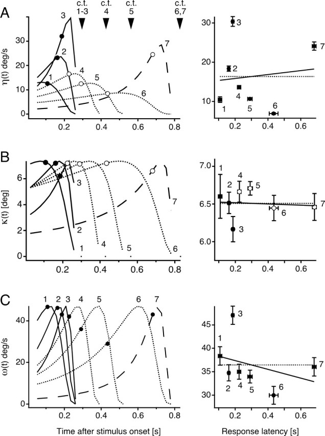
Evaluation of candidate scaling functions at response onset. Left, Time courses of the composite functions η(t) (A), κ(t) (B), and ω(t) (C) for seven different looming stimuli with indicated mean escape latencies for stimuli 1–3 (black dots) and stimuli 4–7 (open circles). The apparent collision time (c.t.) for each stimulus is indicated by an arrowhead. Right, Plots of the mean escape latencies (±SEM, horizontal error bars) versus the mean threshold values at response onset (±SEM, vertical error bars) for stimuli 1–7 (±SEM). The solid black lines indicate the best linear fits of threshold values, whereas dotted lines represent the best horizontal linear fits of the data. Statistical comparison (GEE method and ANOVA) of the threshold values showed significant differences for η(t) and ω but not for κ(t).

Table 1.

Comparison of the values of θth, θ′th, α, β, and ϵ, obtained using two independent methods

	Optimization (means ± SD)	Linear plots
θth (deg)	21 ± 14.4	19.74
θ′th (deg/s)	154 ± 233	35.5
α (deg−1)	0.09 ± 0.011	0.044
β (deg−1)	0.05 ± 0.015	0.0507
ϵ (s·deg−1)	0.0078 ± 0.0033	0.028

Optimization procedure: mean values were calculated by minimizing the variance between estimates extracted from individual response latencies to different stimuli. Linear plots: values were calculated from linear plots of mean latencies across all experiments versus either d/V or (d/V)^1/2, based on the predictions for each function.

Significant differences among the stimuli were observed for η(t) (p < 0.0001) and ω(t) (p = 0.023). The only function that showed no significant differences between its values at response onset was κ(t) (p = 0.36). This finding is also illustrated in the plots of mean parameter values, calculated from individual trials, versus mean latencies for the different stimuli (Fig. 3, right). The κ(t) values are well fit with a horizontal line, whereas the best fits for η(t) and ω(t) are clearly not horizontal. This comparison also holds true for θ(t), θ′(t), and τ(t) (Fig. 2, right). These results suggest that κ(t) is the function that best fits the requirement of a constant value, or threshold, at response onset and therefore may be represented in the visual system or at the M-cell level during object approach.

The optimization procedure used here has one basic assumption, namely that for each candidate function, there is a threshold value (i.e., θth, θ′th, ηth, κth, and ωth) that is the same regardless of the stimulus time course. Hatsopoulos et al. (1995), Sun and Frost (1998), and Gabbiani et al. (1999) derived formulas by which the slopes, S₁ and S₂, of linear plots of the response time (TTC + δ) versus either the ratio of object diameter/approach velocity (d/V) or its square root, (d/V)^1/2, respectively (Fig. 4), can be used to estimate θth, θ′th, and ηth. This method was expanded to include derivations of the values of κth, and ωth. In addition, it is possible to calculate values for the exponential coefficients α, β, and ϵ in the functions η(t), κ(t), and ω(t) for comparison with the results of the optimization procedure. It is based on the condition that that threshold for each composite corresponds to the value of that function at its peak. Indeed, the plots in Figure 3 are consistent which this notion. The specific relationships are as follows:

We first asked whether TTC + δ was linear function d/V or of (d/V)^1/2, and as shown in Figure 4, both fits were satisfactory, with the correlation coefficient for d/V (r = 0.92) being greater than for (d/V)^1/2 (r = 0.88). We then calculated the mean threshold values for θth, θ′th, and the coefficients α, β, and ϵ, for comparison with the values obtained using the optimizing method. Those values are listed in Table 1, and the general correspondence of the results obtained with the two methods provides independent verification of the optimization procedure.

Figure 4.

Quantitative relationships between escape latency and stimulus properties. A, B, Plots of mean escape latency ± SEM, expressed in terms of the TTC versus d/V (A) and (d/V)^1/2 (B), with linear fits. In both, TTC is adjusted by 35 ms (see Materials and Methods). Corresponding slopes, used to calculate values of candidate functions at response onset, and the correlation coefficients are S₁ = 2.873 s·rad⁻¹ (r = 0.921) and S₂ = 1.270 s·rad⁻¹ (r = 0.8840).

Characterization of M-cell responses to looming stimuli

The postulated scaling function κ(t), derived from the behavioral tests, has an expected stimulus-dependent time course that should be reflected in M-cell recordings. Specifically, it predicts that the evoked PSP peaks early and decays while the stimulus continues to grow. The fact that mean escape latency for each stimulus is close to the peak time of the corresponding κ(t) function predicts a similar peak time for the M-cell response. In addition, smaller or faster objects should produce steeper initial PSP growth rates when compared with larger objects approaching at the same velocity (Fig. 3B, left, stimuli 3 vs 1) or with similar-sized objects with slower approach velocities, respectively (Fig. 3B, stimuli 2 vs 6). To test these two predictions, we recorded synaptic responses evoked in the M-cell soma (N = 4) and ventral dendrite (N = 3) by six of the looming stimuli (stimuli 1–6) used in the behavioral experiments. In this case, the fish was fixed in an upright position, with the nose slightly elevated, to facilitate recording from the ventral dendrite, and the trajectory of the simulated approach path was aligned to the center of the head (see also Material and Methods). These stimuli typically evoked bursts of graded PSPs with peak amplitudes up to 9 mV (Fig. 5). The PSP peak times with respect to stimulus onset, which were significantly different for each stimulus (p < 0.001), ranged from 115 to 832 ms and were shorter for faster or larger objects. Moreover, the peak times of the proposed scaling function κ(t), deduced from the behavioral results, and those of the evoked PSP waveforms are highly correlated (R = 0.98) (Fig. 5). A similar correspondence, however, was found for the other candidate composite functions that peak before stimulus offset (η(t), R = 0.98; ω(t), R = 0.99). This agreement suggests that the PSPs in free-swimming fish trigger the M-cell at or close to the peak depolarization. The low incidence of suprathreshold EPSPs, relative to the behavioral response rates, may reflect changes in input resistance associated with the recording itself, given the correspondence between EPSP peak times and behavioral latencies.

Figure 5.

Visual-evoked responses recorded in the M-cell ventral dendrite. As with the behavior, PSPs were evoked by six looming stimuli that either had the same (stimuli 1–3) or different (stimuli 2, 4, and 6) approach speeds. The superimposed black traces represent the corresponding time courses of κ(t), shifted by 25 ms to account for sensory processing time in the visual pathway (Canfield, 2003). The bottom traces indicate the onset and offset of the looming stimuli. The apparent collision time for each stimulus is indicated by an arrowhead. Note difference in time scale for top and bottom traces. The bottom right panel shows the mean PSP peak time (± SEM, vertical error bars) plotted versus the predicted peak times of κ(t) for stimuli 1–6 (14, 24, 13, 14, 13, 30 responses in 5 animals for stimuli 1–6, respectively). Stim., Stimulus.

Each of the electrophysiology experiments included the same control stimuli, as for the behavioral experiments (i.e., receding disks and ones in which the solid black disk was replaced by one with a black and white checkerboard pattern). Figure 6, A1, A2, and B1–B3, illustrates consecutive recordings from two different experiments. Receding disks with an initial angular size of 69° that abruptly appear on the projection screen and become progressively smaller (a reversed stimulus 2) typically evoked no response (Fig. 6A1) or, in a few cases, a small initial response (Fig. 6B2). The corresponding looming responses are shown in Figure 6, A2 and B1 (i.e., they are in the order they were presented). In each case, there was a 1–10 min interval between stimuli. Also, black disks (angular size of 16°) that appeared suddenly and did not move did not evoke any PSPs (data not shown). In contrast, a checkerboard version of an effective looming stimulus evoked PSPs, which had a time course and amplitude very similar to those evoked by the solid black version (Fig. 6, compare B1, B3, stimulus 2).

Figure 6.

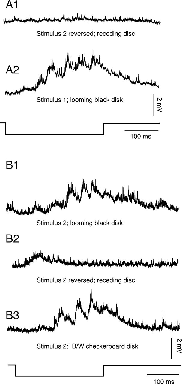
M-cell visual-evoked responses are looming specific. A1, A2, Consecutive traces recorded from an M-cell soma of PSPs evoked by a receding disk (stimulus 2 reversed) and a looming stimulus (stimulus 1), respectively. B1–B3, Successive traces, from another M-cell, of responses to the looming stimulus 2, presented normally, reversed (i.e., receding), and with a checkerboard pattern. In both sets of data, the bottom trace denotes stimulus onset and offset. B/W, Black and white.

To further establish the correspondence between the behavioral results and the predictions for the underlying neural activity in the M-cell, we compared the slopes of individual PSPs recorded in the soma with those of the behaviorally derived κ(t), η(t), and ω(t) functions. The slope of a PSP was calculated between the point of its onset and its peak time, using an automated detection program (Fig. 7A) (see also Material and Methods). As shown in Figure 7B, the steepest slopes for the PSPs and the composite functions were found for stimulus 3, and the normalized slopes covaried over the range of stimuli used. However, in this case, the mean PSP slopes appear most tightly correlated with the slope values predicted by κ(t). To quantify the correspondence between the PSP slopes and the predicted slopes of the candidate scaling functions κ(t), η(t), and ω(t), we compared their estimated standardized distance using the GEE analysis (see Material and Methods). The estimated standardized distance between mean PSP slope and i^th function slopes is D_i = (μ̂ − μ_i)^T ×Σ̂⁻¹ × (μ̂ − μ_i),i = 1,2,3, with μ̂ denoting the estimated mean, Σ̂ denoting the variance–covariance matrix of the PSP slope, and μ₁, μ₂, and μ₃ denoting the slopes for κ(t), η(t), and ω(t), respectively. Here, the superscript T and −1 denote the matrix transpose and inverse, respectively. The resulting distance measures were smallest for κ(t) (885.9), with values of 4156.3 for ω(t) and 41540.5 for η(t), which indicates that the PSP slope is closest to the κ(t) slope.

Figure 7.

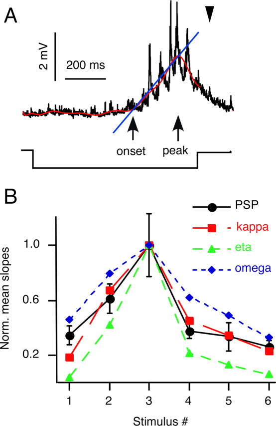
Comparison of rates of rise of evoked PSPs and the corresponding κ(t) functions. A, Sample PSP (top trace) evoked in the M-cell soma by the looming stimulus 6 (black) with corresponding polynomial fit (red). The apparent collision time is indicated by an arrowhead. The individual slopes from PSP onset to PSP peak were calculated using an algorithm (see Material and Methods for details) that detected the onset and peak of the response (black arrows) with respect to a 50 ms baseline before stimulus onset, assuming a linear rise (blue line). Bottom trace, Negative step indicates timing of the stimulus onset and offset. B, Mean values of normalized (Norm.) slopes for the PSPs (± SEM) and for κ(t), η(t), and ω(t) for the six stimuli (9, 12, 7, 14, 5, and 19 responses in 5 animals for stimuli 1–6, respectively).

We asked whether the early peak and subsequent decay of the membrane depolarization despite continued growth of the stimulus might reflect postsynaptic inhibition of the M-cell, for example, by the midbrain interneurons (PHP cells) (Fig. 8A), which provide feedforward afferent inhibition to this neuron (Faber et al., 1991; Wang and Frost, 1992). Individual PHP cells mediate two forms of inhibition, a classical postsynaptic glycinergic shunting inhibition as well as a brief electrical inhibition (Furukawa and Furshpan, 1963; Faber and Korn, 1982). The latter is produced by the currents associated with the presynaptic action potentials in these interneurons and appears as a relatively large extracellular positivity, known as the extrinsic hyperpolarizing potential (EHP) (Fig. 8B) (Faber and Korn, 1978). EHPs can be recorded extracellularly in the neuropil surrounding the initial segment of the M-axon and can be used to monitor the evoked activity of numerous PHP cells. In particular, they are an indicator of the timing of the onset of chemical inhibition in the M-cell. Also, it was shown previously that stimulation of the optic tectum activates PHP cells (Zottoli et al., 1987), as diagrammed in Figure 8A.

Figure 8.

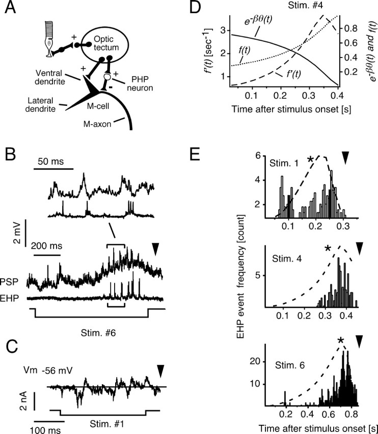
Visual-evoked postsynaptic inhibition. A, Schematic of identified visual system projections to the M-cell including feedforward inhibition mediated by midbrain (PHP) interneurons (Zottoli et al., 1987). B, Simultaneous, intracellular recordings from the M-cell soma and extracellular recordings of visual-evoked presynaptic action potentials from a population of inhibitory PHP cells. The top trace shows an evoked PSP, and the middle trace shows the corresponding train of EHPs in response to a visual looming stimulus. The bottom trace indicates onset and offset of the looming stimulus. The inset (above) is a segment of the same recording on an expanded time scale. C, Voltage-clamp (SEVC) recording from a M-cell depolarized 20 mV from resting potential (300 ms voltage step). Visual evoked IPSCs and EPSCs are indicated by outward and inward currents, respectively. D, Transformation of the experimentally derived scaling function e^−βθ(t)(solid line; β = 0.05) into the inhibitory function f(t) = 1 − e^−βθ(t) (dotted line) and its time derivative f′(t) (dashed line). E, Frequency–time distribution of EHP events evoked by the indicated looming stimuli (total of 9, 11, and 14 responses in 4 animals for stimuli 1, 4, and 6, respectively) with the superimposed time course of f′(t) (dashed lines). * indicates the mean PSP peak time for the three stimuli (data from Fig. 5). The apparent collision time for each stimulus is indicated by an arrowhead. Stim., Stimulus.

An example of EHPs evoked by a visual looming stimulus, together with the simultaneously recorded PSPs in the M-cell, is shown in Figure 8B. It demonstrates that inhibition is distributed throughout the later part of the response, occurring in bursts that are phase shifted relative to the excitatory ones. Similarly, voltage-clamp recordings in the depolarized M-cell (N = 3) revealed IPSCs, which typically were predominant in the later part of the response (Fig. 8C). To quantify looming-evoked inhibition in the M-cell during the period of overlapping excitation, we analyzed the timing of EHP events from four different animals and for three distinct stimuli. The results show that for a given stimulus, inhibition clearly is maximal shortly after the PSP peak is reached (Fig. 8E), although, for larger objects (stimulus 1), inhibition is also potent during the initial part of the response (Fig. 8E, top).

Together, these results imply that inhibition shapes the rising phase of the depolarizing envelope and, hence, would influence when the M-cell reaches threshold and triggers the behavior. Also, the late onset of massive postsynaptic inhibition plays a major role in terminating the excitatory postsynaptic response. A quite similar role of inhibition has been described recently for a looming sensitive neuron in locust (Gabbiani et al., 2005). Moreover, these results raise the possibility that the implementation of the observed neural transformation of looming information depends on postsynaptic inhibitory input to the M-cell. In other words, the progressive attenuation of excitation attributed to the scaling function could be explained by an inhibitory factor, f(t), which ranges from zero to one. This concept can be expressed by the transformation κ(t) = θ(t − δ) × e^{−βθ(t − δ)} = θ(t) − (θ(t) × f(t)), where f(t) = 1 − e^{−βθ(t − δ)} and grows nonlinearly with stimulus size (Fig. 8D). This inhibition of the M-cell would be a consequence of the presynaptic activity in the PHP cells; theoretically, f(t) is caused by the convolution of the unitary presynaptic impulses and the corresponding inhibitory conductance changes they produce. If we approximate the conductance changes, which last >10 ms (Faber and Korn, 1988), as step functions, the first derivative f′(t) can be used to estimate the expected time course of the presynaptic inhibitory volley (Fig. 8D).

For each stimulus, the time courses of f(t) and f′(t) were derived from the experimentally determined κ(t) (Fig. 8D), and f′(t) is superimposed on the frequency–time distribution of the evoked EHPs in Figure 8E. The apparent correspondence between the peaks of the predicted and the measured inhibitory activity suggests the brainstem inhibitory interneurons (PHP cells) are the source of the postsynaptic inhibition. Because f′(t) ∼ θ′(t), this result also suggests that impulses in these interneurons encode a function of angular velocity, which is integrated at the M-cell level into a scaled function of view angle.

Discussion

Our results provide insights that link integrative events at the cellular, synaptic, and network levels to a defined natural behavior. First, they demonstrate that the M-cell itself is implicated in the final computation of stimulus features, despite the earlier stages of information processing in the retina and optic tectum. Second, a quantitative analysis of the behavior, specifically of its latency relative to stimulus size and dynamics, is sufficient to predict the stimulus representation at the level of the M-cell (i.e., the putative decision-making neuron for the observed behavior). Third, inhibition at this final stage influences both the time course and magnitude of excitation of the M-cell, implying that it may also influence the behavioral threshold and timing of the escape.

M-cell triggered escapes to visual stimuli

We show here that the goldfish M-cells initiate visual-evoked escapes, or C-starts. Although escape behaviors to looming stimuli were described previously in other fish species (Dill, 1974; Webb, 1986; Batty, 1989), it was not clear whether these responses were initiated by the M-cell or by a network of other descending brainstem neurons (Fetcho, 1991; Nakayama and Oda, 2004). M-cell-initiated C-starts have been typically associated with abrupt mechanosensory stimuli (Zottoli, 1977; Eaton et al., 1981; Preuss and Faber, 2003). Thus, the involvement of this neuron in escapes in response to gradual, complex visual stimuli adds to its potential for understanding mechanisms of sensory integration in a single neuron (for recent review, see Koch and Segev, 2000). For example, our results also indicate that abrupt visual stimuli, such as the sudden display of a black disk, are ineffective in eliciting a behavioral response. Similarly ineffective are strobe flashes (data not shown). Sound-evoked escapes have latencies in the range of 10–15 ms, more than an order of magnitude faster than the escapes described here. As noted, mechanosensory and visual inputs impinge on different dendrites of the M-cell, and it is likely that the two dendrites process inputs in different time domains.

Quantitative correlation between behavior and physiology

One potentially confounding factor in interpreting M-cell responses in restrained fish to “natural stimuli” that evoke escapes in free-swimming fish is that in the former condition, the cell does not reach threshold for firing an action potential. This is the case for all modes of stimulation that can evoke escapes (Preuss and Faber, 2003). This discrepancy presumably reflects a decreased excitability of the system in the conditions used for electrophysiology, rather than damage to the M-cell, because M-cell spikes were not observed with the same stimuli during the extracellular recordings of the presynaptic inhibitory activity. Nevertheless, when behavior and electrophysiology are compared, for both visual and auditory (Preuss and Faber, 2003), the timing of the PSPs is as predicted, suggesting that either the M-cell is more hyperpolarized in restrained fish or additional depolarizing inputs are not being activated.

It should be stressed that we took a different approach to the problem that both the observed behavior and the M-cell PSPs occur with a time lag with respect to the driving function (i.e., the dynamics of the visual image on the retina). Whereas other investigators have estimated that time lag, δ, from their recordings (Sun and Frost, 1998, Gabbiani et al., 1999), we have rather chosen to use a value based on known delays in the sensory and motor pathways. Also, we adopted the earlier assumption that δ is a constant regardless of the specific features of the visual stimulus. However, in reality, δ is more likely to vary, because the time delay from the retina to the optic tectum and hence to the M-cell is presumably not a constant.

Implementation of the exponential scaling function

In a first approximation, our behavioral results might suggest that escape onset is related to a distinct threshold value of angular retinal image size, θ(t) or its expansion velocity, θ′(t) of the looming stimulus. Previous quantitative behavioral studies in a number of animals describe angular threshold values, in a similar size range of 10–35° (Schiff 1965; Robertson and Johnson, 1993; Yamamoto et al., 2003). However, our statistical analysis shows that neither θ(t) nor θ′(t) by itself can fully account for the observed behavioral latencies over the tested range of looming stimuli. Instead, our results suggest that a refined (i.e., dynamically scaled) function of angular size determines the escape onset in goldfish. This finding is further supported by the electrophysiological results. Indeed, the stimulus waveform predicted by the proposed scaling function, namely κ(t), has a stimulus specific slope and peak time that closely resembles the recorded PSP waveform in the threshold detector, the M-cell.

This scaling can be understood as a dynamic nonlinear process that gives added weight to θ(t) initially and deemphasizes it with time. In principle, such scaling can be implemented by a nonlinear interaction of, for example, excitatory and inhibitory signals that both track θ(t). A very similar scaling function, namely η(t), has been suggested for the responses of looming sensitive neurons in the nucleus rotundus in pigeons (Sun and Frost, 1998) and the lobula giant movement detector of locust (Hatsopoulos et al. 1995). In these cases, however, the scaled parameter is θ′(t) instead of θ(t). This apparent discrepancy could be reconciled by the notion that upstream neurons in the visual pathway commonly code θ′(t), which subsequently is integrated by downstream neurons such as the M-cell to θ(t).

Thus, the major finding presented here is that the better descriptor of the behavior and its electrophysiological correlates is a function that peaks before stimulus offset, as opposed to functions that are directly proportional to θ or θ′. In this context, η(t), κ(t), and ω(t) all fall into the same class of scaling function, with κ(t) being more satisfactory statistically for the range of looming stimuli tested.

Together, the results imply that the characteristics of a looming stimulus are encoded at the population level, that is, in the firing patterns of those tectal afferents that converge onto the ventral dendrite of the M-cell (Zottoli et al., 1987) and those that innervate a specific class of premotor inhibitory interneurons (Faber and Korn, 1978; Faber et al., 1991). Although our results are only correlative, they are consistent with the idea that subsequent spatial and temporal integration of these inputs in the M-cell, the downstream decision-making neuron, provides the basis for the rise-to-threshold mechanism that functionally decodes the looming information and transforms it into a critically timed motor command. Timing and magnitude of postsynaptic inhibition guide temporal aspects of the decoding process. These findings underline the important role that even single neurons can play in sensorimotor integration of complex information and provide a practical example for neural decision-making.

The proposed scaling function can be understood as the difference between an excitatory signal, θ(t), and an inhibitory function that depends on the multiplication of two size-dependent factors, that is, θ(t) and f(t), where the latter equals 1 − e^{−βθ(t − δ)}. Because of the exponential in the latter term, the inhibition becomes disproportionally large as stimulus size increases, whereas the excitatory term linearly tracks object size. Our physiological results suggest that inhibition and excitation converge at the M-cell. That is, the neural implementation of the scaling function would be consistent with the subtraction of the inhibitory signal from the excitatory one at this level. Computing the magnitude of the inhibition requires a multiplicative step. This operation would appear to be best implemented by shunting inhibition or in neurons with nonlinear membrane properties (Koch, 1998). Although the present results favor a role of shunting inhibition, other nonlinearities have been reported for the M-cell as well, in particular a voltage dependence of activated glycine receptor channels that enhances inhibition evoked during depolarization (Faber and Korn, 1987). A conceptually similar multiplicative interaction in a single neuron has been proposed previously in the lobular giant motion detector of locust (Gabbiani et al., 2002, 2005). Nevertheless, in the case of the M-cell, it remains possible that these operations are in part implemented in the optic tectum and reflect inhibition there (Sajovic and Levinthal, 1983).

Functional consequences

What possible role does the neural transformation (i.e., the proposed inhibitory scaling) have for the expression of the behavior and for detecting and tracking an approaching object? This inhibition causes a distinct peak and attenuation of the integrated synaptic response before stimulus offset, which may contribute to behavioral variability, because it also provides the basis for a fraction of events in which the animal instead does not respond. This unpredictability could add survival value, compared with escapes that are deterministic and stereotyped (Driver and Humphries, 1988; Arnott et al., 1999; Matheson et al., 2004). Moreover, a scaling function such as κ(t) enhances the sensitivity to small (far away) approaching objects and prevents saturation as the object grows (i.e., gets closer). A consequence of the nonlinearity in the neural transformation is that the overall stimulus representation peaks before the end of the stimulus, with the peak time being earlier for faster or larger objects. In functional terms, it effectively accentuates the salience of a potential threat in the early phase of approach and presumably increases the likelihood of an appropriately timed escape.

References

- Arnott SA, Neil DM, Ansell AD (1999). Escape trajectories of the brown shrimp Crangon Crangon, and a theoretical consideration of initial escape angles from predators. J Exp Biol 202:193–209. [DOI] [PubMed] [Google Scholar]
- Batty RS (1989). Escape responses of herring larvae to visual stimuli. J Mar Biol Ass UK 69:647–654. [Google Scholar]
- Canfield JG (2003). Temporal constraints on visually directed C-start responses: behavioral and physiological correlates. Brain Behav Evol 61:148–158. [DOI] [PubMed] [Google Scholar]
- Dill LW (1974). The escape response of the zebra danio (Brachydanio Rerio) I. The stimulus for escape. Anim Behav 22:711–722. [Google Scholar]
- Driver PM, Humphries DA (1988). In: Protean behaviour: the biology of unpredictability Oxford: Clarendon.
- Eaton RC, Lavender WA, Wieland CM (1981). Identification of Mauthner-initiated patterns in goldfish: evidence from simultaneous cinematography and electrophysiology. J Comp Physiol A Neuroethol Sens Neural Behav Physiol 144:521–531. [Google Scholar]
- Faber DS, Korn H (1978). In: Neurobiology of the Mauthner cell pp. 47–126. New York: Raven.
- Faber DS, Korn H (1982). Transmission at a central inhibitory synapse. I. Magnitude of the unitary postsynaptic conductance change and kinetics of channel activation. J Neurophysiol 48:654–678. [DOI] [PubMed] [Google Scholar]
- Faber DS, Korn H (1987). Voltage-dependence of glycine-activated Cl− channels: a potentiometer for inhibition? J Neurosci 7:807–811. [DOI] [PMC free article] [PubMed] [Google Scholar]
- Faber DS, Korn H (1988). Unitary conductance changes at the teleost Mauthner cell glycinergic synapses: a voltage clamp and pharmacologic analysis. J Neurophysiol 60:1982–1999. [DOI] [PubMed] [Google Scholar]
- Faber DS, Korn H, Lin JW (1991). Role of medullary networks and postsynaptic membrane properties in regulating Mauthner cell responsiveness to sensory excitation. Brain Behav Evol 37:286–297. [DOI] [PubMed] [Google Scholar]
- Fetcho JR (1991). Spinal network of the Mauthner cell. Brain Behav Evol 37:298–316. [DOI] [PubMed] [Google Scholar]
- Foreman MB, Eaton RC (1993). The direction change concept for reticulospinal control of goldfish escape. J Neurosci 13:4101–4113. [DOI] [PMC free article] [PubMed] [Google Scholar]
- Furukawa T, Furshpan EJ (1963). Two inhibitory mechanisms in the Mauthner neurons of goldfish. J Neurophysiol 26:140–176. [DOI] [PubMed] [Google Scholar]
- Gabbiani F, Krapp HG, Laurent G (1999). Computation of object approach by a wide-field, motion-sensitive neuron. J Neurosci 19:1122–1141. [DOI] [PMC free article] [PubMed] [Google Scholar]
- Gabbiani F, Mo C, Laurent GJ (2001). Invariance of angular threshold computation in a wide-field looming-sensitive neuron. Neuroscience 21:314–329. [DOI] [PMC free article] [PubMed] [Google Scholar]
- Gabbiani F, Krapp HG, Koch C, Laurent G (2002). Multiplicative computation in a visual neuron sensitive to looming. Nature 420:320–324. [DOI] [PubMed] [Google Scholar]
- Gabbiani F, Cohen I, Laurent G (2005). Time-dependent activation of feed-forward inhibition in a looming-sensitive neuron. J Neurophysiol 94:2150–2161. [DOI] [PMC free article] [PubMed] [Google Scholar]
- Gibson JJ (1961). Ecological optics. Vision Res 1:253–262. [Google Scholar]
- Gibson JJ (1979). In: The ecological approach to visual perception Boston: Houghton Mifflin.
- Hatsopoulos N, Gabbiani F, Laurent G (1995). Elementary computation of object approach by a widefield visual neuron. Science 270:1000–1003. [DOI] [PubMed] [Google Scholar]
- Holmqvist MH, Srinivasan MV (1991). A visually evoked escape response of the housefly. J Comp Physiol A Neuroethol Sens Neural Behav Physiol 169:1432–1451. [DOI] [PubMed] [Google Scholar]
- Koch C (1998). In: Biophysics of computation: information processing in single neurons, Chap 20 pp. 469–477. Oxford: Oxford UP.
- Koch C, Segev I (2000). The role of single neurons in information processing. Nat Neurosci 3:1171–1177. [DOI] [PubMed] [Google Scholar]
- Korn H, Faber DS (2005). The Mauthner cell half a century later: a neurobiological model for decision-making? Neuron 47:13–28. [DOI] [PubMed] [Google Scholar]
- Laurent G, Gabbiani F (1998). Collision-avoidance: nature's many solutions. Nat Neurosci 1:261–263. [DOI] [PubMed] [Google Scholar]
- Liang KY, Zeger SL (1986). Longitudinal data analysis using generalized linear models. Biometrika 73:13–22. [Google Scholar]
- Matheson T, Rogers SM, Krapp HG (2004). Plasticity in the visual system is correlated with a change in lifestyle of solitarious and gregarious locusts. J Neurophysiol 91:1–12. [DOI] [PubMed] [Google Scholar]
- McCullagh P, Nelder JA (1989). In: Generalized linear models Ed 2 Oxford: Chapman and Hall.
- Nakayama H, Oda Y (2004). Common sensory inputs and differential excitability of segmentally homologous reticulospinal neurons in the hindbrain. J Neurosci 24:3199–3209. [DOI] [PMC free article] [PubMed] [Google Scholar]
- Preuss T, Faber DS (2003). Central cellular mechanisms underlying temperature-dependent changes in the goldfish startle-escape behavior. J Neurosci 23:5617–5626. [DOI] [PMC free article] [PubMed] [Google Scholar]
- Regan D (2002). Binocular information about time to collision and time to passage. Vision Res 42:2479–2484. [DOI] [PubMed] [Google Scholar]
- Regan D, Vincent A (1995). Visual processing of looming and time to contact throughout the visual field. Vision Res 35:1845–1857. [DOI] [PubMed] [Google Scholar]
- Rind CF, Santer RD (2004). Collision avoidance and a looming sensitive neuron: size matters but biggest is not necessarily best. Proc R Soc Lond B Suppl 271: pp. S27–S29. [DOI] [PMC free article] [PubMed] [Google Scholar]
- Rind FC, Simmons PJ (1992). Orthopteran DCMD neuron: a reevaluation of responses to moving objects. I Selective responses to approaching objects. J Neurophysiol 68:1654–1666. [DOI] [PubMed] [Google Scholar]
- Rind FC, Simmons PJ (1996). Seeing what is coming: building collision-sensitive neurons. Trends Neurosci 22:215–220. [DOI] [PubMed] [Google Scholar]
- Robertson RM, Johnson AG (1993). Retinal image size triggers obstacle avoidance in flying locust. Naturwissenschaften 80:176–178. [Google Scholar]
- Sajovic P, Levinthal C (1983). Inhibitory mechanism in zebrafish optic tectum: visual response properties of tectal cells altered by picrotoxin and bicuculline. Brain Res 271:227–240. [DOI] [PubMed] [Google Scholar]
- Schiff W (1965). Perception of impending collision: a study of visually directed avoidant behavior. Psychol Monogr 79:1–26. [DOI] [PubMed] [Google Scholar]
- Sun H, Frost BJ (1998). Computation of different optical variables of looming objects in pigeon nucleus rotundus neurons. Nat Neurosci 1:296–303. [DOI] [PubMed] [Google Scholar]
- Tresilian JR (1999). Visually timed action: time-out for ‘tau'? Trends Cogn Sci 3:301–309. [DOI] [PubMed] [Google Scholar]
- Trevarthen C (1968). Vision in fish: the origins of the visual frame for action in vertebrates. In: The central nervous system and fish behaviour (Ingle D, ed.) pp. 61–94. Chicago: University of Chicago.
- Wang Y, Frost BJ (1992). Time to collision is signaled by neurons in the nucleus rotundus of pigeons. Nature 356:236–238. [DOI] [PubMed] [Google Scholar]
- Wang Y, Jiang S, Frost BJ (1993). Visual processing in pigeon nucleus rotundus: luminance, colour, motion, and looming subdivisions. Vis Neurosci 10:21–31. [DOI] [PubMed] [Google Scholar]
- Webb PW (1986). Effect of body form and response threshold on the vulnerability of four species of teleost prey attacked by largemouth bass (Micropterus salmoides). Can J Fish Aquat Sci 43:763–771. [Google Scholar]
- Wicklein M, Strausfeld NJ (2000). Organization and significance of neurons that detect change of visual depth in the hawk month Manduca sexta J Comp Neurol 424:356–376. [PubMed] [Google Scholar]
- Yamamoto K, Nakata M, Nakagawa H (2003). Input and output characteristics of collision avoidance behavior in the frog Rana catesbeiana Brain Behav Evol 62:201–211. [DOI] [PubMed] [Google Scholar]
- Zottoli SJ (1977). Correlation of the startle reflex and Mauthner cell auditory responses in unrestrained goldfish. J Exp Biol 66:243–254. [DOI] [PubMed] [Google Scholar]
- Zottoli SJ, Faber DS (2000). The Mauthner cell: what has it taught us? The Neuroscientist 6:26–38. [Google Scholar]
- Zottoli SJ, Hordes AR, Faber DS (1987). Localization of optic tectal input to the ventral dendrite of the goldfish Mauthner cell. Brain Res 401:113–121. [DOI] [PubMed] [Google Scholar]
- Zottoli SJ, Bentley AP, Prendergast BJ, Rieff HI (1995). Comparative studies on the Mauthner cell of teleost fish in relation to sensory input. Brain Behav Evol 46:151–164. [DOI] [PubMed] [Google Scholar]