

Abstract
Objective
Tuberculosis (TB) remains a major deadly threat in mainland China. Early warning and advanced response systems play a central role in addressing such a wide-ranging threat. The purpose of this study is to establish a new hybrid model combining a seasonal autoregressive integrated moving average (SARIMA) model and a non-linear autoregressive neural network with exogenous input (NARNNX) model to understand the future epidemiological patterns of TB morbidity.
Methods
We develop a SARIMA-NARNNX hybrid model for forecasting future levels of TB incidence based on data containing 255 observations from January 1997 to March 2018 in mainland China, and the ultimate simulating and forecasting performances were compared with the basic SARIMA, non-linear autoregressive neural network (NARNN) and error-trend-seasonal (ETS) approaches, as well as the SARIMA-generalised regression neural network (GRNN) and SARIMA-NARNN hybrid techniques.
Results
In terms of the root mean square error, mean absolute error, mean error rate and mean absolute percentage error, the identified best-fitting SARIMA-NARNNX combined model with 17 hidden neurons and 4 feedback delays had smaller values in both in-sample simulating scheme and the out-of-sample forecasting scheme than the preferred single SARIMA(2,1,3)(0,1,1)12 model, a NARNN with 19 hidden neurons and 6 feedback delays and ETS(M,A,A), and the best-performing SARIMA-GRNN and SARIMA-NARNN models with 32 hidden neurons and 6 feedback delays. Every year, there was an obvious high-risk season for the notified TB cases in March and April. Importantly, the epidemic levels of TB from 2006 to 2017 trended slightly downward. According to the projection results from 2018 to 2025, TB incidence will continue to drop by 3.002% annually but will remain high.
Conclusions
The new SARIMA-NARNNX combined model visibly outperforms the other methods. This hybrid model should be used for forecasting the long-term epidemic patterns of TB, and it may serve as a beneficial and effective tool for controlling this disease.
Keywords: tuberculosis, forecasting, statistics, models
Strengths and limitations of this study.
This work showed the long-term temporal patterns and characteristics in tuberculosis (TB) incidence series through a 29-year analysis.
The seasonal autoregressive integrated moving average-non-linear autoregressive neural network with exogenous input (SARIMA-NARNNX) hybrid model can be employed to implement long-term forecasting of TB in mainland China.
The time variable is a significantly useful parameter that fails to be ignored during the process of constructing prediction models, particularly when a clear seasonality is included in the time series.
The SARIMA-NARNNX hybrid model has the potential for far-reaching implications for further prevention and control of TB incidence.
The SARIMA-NARNNX hybrid model only relies on the retrospective responses and time factors without considering additional explanatory variables.
Introduction
Tuberculosis (TB) is a worldwide chronic infectious disease caused by the aetiological agent Mycobacterium tuberculosis that is usually spread among people through direct and indirect contact by droplets, droplet nuclei and dust.1 Infection is typically found in the lungs but can also affect other organs.2 At present, although great progress has been made around the world in the prevention and control of TB, many countries, especially in low-income and middle-income settings, are still afflicted with a chronic plague of TB with huge losses to their economies, with funding reaching US$6.9 billion in 2018.3 4 Moreover, TB is among the top 10 causes of death worldwide; it is estimated that globally there were 10.0 million new cases of TB in 2017, of which 1.3 million individuals’ deaths were directly attributable to TB, and TB has killed more people than any other infectious disease in the past few decades.2 5 The eight countries that were hit the hardest with TB in 2017 (China ranked second) accounted for two-thirds of the global burden of TB.2 During the same period, China recorded the second largest morbidity of multidrug-resistant TB (MDR-TB) cases with an estimated 778 390 new TB notifications.2 Furthermore, the costs of each confirmed case of TB have reached as much as 2% of urban residents’ average annual income in mainland China.6 Currently, although the TB incidence has been slightly decreasing annually in mainland China,7 the potential achievement is diminished by an increasing large-scale transient population, the emergence of MDR-TB, along with the comorbid conditions of AIDS and non-communicable diseases, which have led to a resurgence of TB in many regions in recent years.2 8 9 Additionally, WHO initiated the End TB Strategy in 2014 with the target of a 90% reduction in new TB cases by 2035 compared with 2015 and a milestone of reducing the TB incidence rate by 50% by 2025 relative to 2015.10 To accelerate progress towards such a daunting task, corresponding measures and actions are expected at both the national and international levels. At the national level, appropriate plans can fail to be becomingly formulated without getting a clear perspective of the past, current and future temporal levels of this disease. Therefore, advanced detection and early response systems for epidemics have formed an integral part of the effective precautions against TB and the reasonable allocation of available health resources.
Currently, numerous useful statistical techniques have been extensively employed in the forecasting domain, including linear methods such as the seasonal autoregressive integrated moving average (SARIMA) method,9 the error-trend-seasonal (ETS) approach,11 linear regression,12 support vector machines12 and autoregressive distributed-lag modelling13; non-linear models, predominantly involving artificial neural networks (ANNs)14and linear and the non-linear hybrid methods.7 13 15 Whereas complexities and challenges in understanding the incidence trends of infectious diseases are the linear and non-linear interactions among different dimensions in real-world scenarios.14 16 Consequently, hybrid models comprising the SARIMA model and generalised regression neural networks (GRNNs) as well as non-linear autoregressive neural network (NARNN) techniques that can enable arbitrarily intricate non-stationary series to attain any desired accuracy owing to their powerful flexible non-linear mapping capacity and accomplish satisfactory performance in epidemiological predictions.3 9 14–19 It has been shown that the SARIMA-NARNN combined model can provide a more accurate insight into time-dependent data than the SARIMA-GRNN hybrid model.20 However, the time variable is fairly helpful in modelling long-trajectory data exhibiting obvious seasonality and cyclicity,3 14 20 21 which is invariably neglected during SARIMA-NARNN model development.9 Importantly, many studies have confirmed that TB morbidity manifests obvious seasonal and cycle patterns.3 7 14 15 22 Therefore, to take full advantage of the linear and non-linear components hidden in the epidemiological data, our team first proposes a hybrid methodology based on the SARIMA model and the non-linear autoregressive neural network with exogenous input (NARNNX) for modelling the long-term seasonality and forecasting trends in TB incidence, called SARIMA-NARNNX. To further test and verify the feasibility and flexibility of this hybrid technique, the single SARIMA, NARNN and ETS methods, coupled with the traditional SARIMA-GRNN and SARIMA-NARNN hybrid techniques, were also established to simulate the TB incidence data, and then their modelling and forecasting powers were compared with our proposed hybrid model to find the optimal model to make a contribution to the elimination of TB in China and worldwide.
Materials and methods
Data sources
In this observational study, the longitudinal monthly morbidity data from January 1997 to March 2018 were extracted from the notifiable infectious disease reporting system supplied by the Chinese Center for Disease Control and Prevention (http://www.nhfpc.gov.cn/jkj/s2907/new_list_6.shtml) and the disease surveillance website (http://www.jbjc.org/CN/article/showVolumnList.do). A total of 255 months of observations over a period of 22 years were obtained for the analysis. Subsequently, the data were separated into two groups; the first 240 points were designated for in-sample model building, while the remaining 15 points were reserved for forecasting assessment and comparison (online supplementary table S1).
bmjopen-2018-024409supp001.pdf (819.3KB, pdf)
Statistical analysis
Developing the SARIMA-NARNNX hybrid model
The NARNN model only uses the known past input values to estimate the present output results (online supplementary figure S1), which may influence its prediction and extrapolation accuracies because the time variable is a significant rewarding parameter that fails to be ignored, particularly when a clear seasonality is present in the time series.9 In addition, there are strong correlations between the fitted values of the SARIMA model and the actual values of TB morbidity sequences. Therefore, the importance of the time variable is highlighted in our proposed SARIMA-NARNNX hybrid model. The time variable and the estimated values of the SARIMA model were regarded as input variables in our model, while the corresponding TB reported cases were used as the output variable (online supplementary figure S2). Then, the informative linear and non-linear implications contained in the TB notification data are systematically excavated through this combined methodology. Finally, the best-fitting hybrid model identified is employed to conduct out-of-sample predictions. The estimated equation of the SARIMA-NARNNX combined model is defined as
| (1) |
Here, f represents a function that relies on the structure and connection weights of the NARNNX model, signifies the simulated and projected values from the hybrid technique, y refers to the given prior TB incidence data in a lagged period d, and x denotes the input values containing the time factor and the mimics and projections of the SARIMA method.
In this hybrid model, the modelling steps were as follows. Initially, as mentioned above, the time variable and the estimated values of the SARIMA model were regarded as input variables, while the corresponding reported cases of TB were used as the output variable. Subsequently, the random divider and function was applied to classify the in-sample data into three subsets: a training dataset (80% of the data), a validation dataset (10%) and a testing dataset (10%). Then, the number of hidden neurons and delays d was adjusted by trial and error using the Levenberg-Marquardt algorithm in an open feedback loop mode. The response plot of the outputs and targets and the residual autocorrelation function (ACF) plot, together with the mean square error (MSE) and correlation coefficient (R), were used to find the best-performing SARIMA-NARNNX model. Finally, the training open-loop architecture was transformed into closed-loop mode to make multistep-ahead forecasts (The code used in our experiments is included in the online supplementary materials).
Moreover, the single SARIMA and the traditional SARIMA-GRNN and SARIMA-NARNN models were constructed as described in the online supplementary materials, and their modelling and forecasting powers were compared with the SARIMA-NARNNX hybrid model.
Performance measures among models
In this work, the SARIMA model was built with the R statistical package (V.3.4.3, R Development Core Team, Vienna, Austria), and the selected three hybrid models, including the SARIMA-GRNN, SARIMA-NARNN and SARIMA-NARNNX, were developed with MATLAB (V.R2014a, MathWorks, Natick, Massachusetts, USA). A two-sided p <0.05 was considered statistically significant.
Of the mathematical methodologies mentioned above, the mimic and predictive performances were judged by two types of measures: scale-dependent indices (ie, the root mean square error (RMSE) and the mean absolute error (MAE)) and indices that depend on percentage errors (ie, the mean error rate (MER) and the mean absolute percentage error (MAPE)). For these measures, the smallest values correspond to the optimal method.
| (2) |
| (3) |
| (4) |
| (5) |
where Xi denotes the observed values, signifies the simulated and projected values from the four selected models, represents the average of the observed values, and N is the number of fitted or projected values from the four selected models.
Patient and public involvement
Patients and the public were not involved in our present study, as the TB incidence series from the notifiable infectious disease reporting system was aggregated as secondary data and does not contain personal identifying information. Thus, these data are publicly available.
Results
General information
A total 17 926 271 cases were reported during the period between January 1997 and March 2018, with a monthly average morbidity of 88 304 cases, resulting in a yearly average incidence rate of 63.724 cases per 100 000 people. The incidence rate has remarkably risen from 30.836 cases per 100 000 persons in 1997 to 60.082 cases per 100 000 persons in 2017, with an increase of 94.847%. The highest incidence peak was at a maximum in 2005 with 96.310 cases per 100 000 population, which was a marginal increase of 212.332% compared with 2008 (online supplementary figure S3). When the short-term monthly effects of TB morbidity from January 1997 to March 2018 were removed by the Hodrick-Prescott (HP) decomposition approach (figure 1), it was observed that there are apparent seasonal peak activities in the TB incidence time series, especially in March and April of each year, and the seasonal periodicity continued to fluctuate with a length of 12 months. In addition, the TB case notifications from 2006 to 2017 trended slightly downward but were still significantly high.
Figure 1.
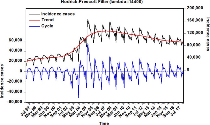
Decomposition of monthly TB time series in mainland China from 1997 to 2018 into trend and cyclical components using the Hodrick-Prescott filter. TB, tuberculosis.
The best-performing SARIMA model
Before modelling, an augmented Dickey-Fuller (ADF) test was performed in the reported TB incidence series that indicated that the data are irregular and non-stationary (ADF=−1.705, p=0.427). Consequently, according to the results of the ADF test and TB incidence periodicity, the first-order seasonal and non-seasonal differences were taken to remove the instabilities in the variance and mean (ADF=−4.175, p<0.001), which indicated that the differenced series was stationary. Subsequently, by analysing the spikes of the ACF and partial ACF (PACF) plots from the transformed TB morbidity series (online supplementary figures S4 and S5), several candidate models were roughly chosen to further discover the optimal SARIMA model (online supplementary table S2). Next, the best-performing SARIMA(2,1,3)(0,1,1)12 model was selected based on the residual correlations in both the ACF and PACF plots, as well as the akaike information criterion (AIC), bias-corrected AIC (AICc) and schwarz bayesian criterion (SBC) values. The AIC, AICc and SBC values of 4914.44, 4914.94 and 4938.60, respectively, were the smallest among those candidate models. The ACF and PACF residual plots demonstrated that the error correlations at lags almost fell into the estimated threshold limits, and the Ljung-Box Q-test also revealed that the residuals were a white noise series (figure 2 and table 1). Furthermore, the testing results of the estimated parameters were all statistically significant. Nevertheless, the lagrangian multiplier (LM) test demonstrated that apparent autoregressive conditional heteroscedastic (ARCH) effects were noted at different lags in the residual series (table 2). The specified equation of the SARIMA(2,1,3)(0,1,1)12 model can be written as (1-B)(1-B)12 Xt=(1+2.161B-1.938B2 +0.633B3 (1+0.7B12 ɛt/(1–1.52B+0.909B2). Ultimately, the preferred model can be applied to predict the incident cases from January 2017 to March 2018 (table 3).
Figure 2.
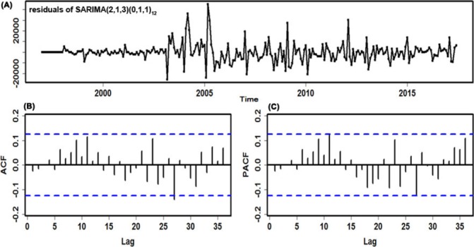
Diagnostic checking for the residuals generated by the SARIMA(2,1,3)×(0,1,1)12 method. (A) Standardised residual plot; (B) autocorrelation function (ACF) of the errors at various lags; (C) Partial ACF (PACF) of the errors at various lags. SARIMA, seasonal autoregressive integrated moving average.
Table 1.
Ljung-Box Q tests of the errors series for the chosen best-undertaking methods at different lags
| Lags | SARIMA | SARIMA-GRNN | SARIMA-NARNN | SARIMA-NARNNX | ||||
| Box-Ljung Q | P value | Box-Ljung Q | P value | Box-Ljung Q | P value | Box-Ljung Q | P value | |
| 1 | 0.079 | 0.779 | 2.287 | 0.130 | 1.769 | 0.183 | 0.057 | 0.811 |
| 3 | 0.084 | 0.994 | 3.308 | 0.347 | 6.010 | 0.111 | 0.336 | 0.953 |
| 6 | 0.970 | 0.987 | 3.969 | 0.681 | 7.375 | 0.288 | 0.436 | 0.999 |
| 9 | 4.065 | 0.907 | 4.850 | 0.847 | 8.940 | 0.443 | 1.348 | 0.998 |
| 12 | 7.396 | 0.830 | 6.097 | 0.911 | 10.706 | 0.554 | 3.160 | 0.994 |
| 15 | 8.480 | 0.903 | 7.667 | 0.936 | 14.006 | 0.525 | 5.059 | 0.992 |
| 18 | 9.763 | 0.939 | 11.351 | 0.879 | 14.478 | 0.697 | 9.189 | 0.955 |
| 21 | 10.959 | 0.964 | 11.446 | 0.953 | 14.997 | 0.823 | 10.320 | 0.975 |
| 24 | 15.399 | 0.909 | 17.626 | 0.821 | 17.174 | 0.841 | 18.569 | 0.775 |
| 27 | 20.056 | 0.828 | 21.015 | 0.786 | 19.064 | 0.868 | 30.082 | 0.311 |
| 30 | 20.803 | 0.894 | 21.071 | 0.886 | 20.029 | 0.916 | 33.156 | 0.316 |
| 33 | 23.485 | 0.889 | 22.172 | 0.924 | 21.507 | 0.938 | 38.354 | 0.240 |
| 36 | 25.866 | 0.894 | 25.066 | 0.914 | 22.383 | 0.963 | 40.113 | 0.293 |
GRNN, generalised regression neural network; NARNN, non-linear autoregressive neural network; NARNNX, non-linear autoregressive neural network with exogenous input; SARIMA, seasonal autoregressive integrated moving average.
Table 2.
ARCH effects of the observations and errors series for the chosen best-undertaking method at various lags
| Lags | Original values | SARIMA | SARIMA-GRNN | SARIMA-NARNN | SARIMA-NARNNX | |||||
| LM-test | P value | LM-test | P value | LM-test | P value | LM-test | P value | LM-test | P value | |
| 1 | 192.37 | <0.001 | 44.973 | <0.001 | 58.393 | <0.001 | 5.522 | 0.019 | 0.358 | 0.550 |
| 3 | 192.95 | <0.001 | 47.413 | <0.001 | 67.078 | <0.001 | 6.659 | 0.084 | 4.639 | 0.200 |
| 6 | 190.52 | <0.001 | 46.980 | <0.001 | 66.140 | <0.001 | 8.581 | 0.199 | 4.791 | 0.571 |
| 9 | 192.910 | <0.001 | 46.254 | <0.001 | 65.552 | <0.001 | 9.030 | 0.435 | 5.654 | 0.774 |
| 12 | 199.100 | <0.001 | 71.910 | <0.001 | 71.985 | <0.001 | 11.386 | 0.496 | 7.08 | 0.852 |
| 15 | 203.180 | <0.001 | 72.409 | <0.001 | 71.654 | <0.001 | 11.841 | 0.691 | 8.205 | 0.915 |
| 18 | 200.2 | <0.001 | 71.245 | <0.001 | 71.075 | <0.001 | 12.991 | 0.792 | 9.272 | 0.953 |
| 21 | 197.06 | <0.001 | 70.719 | <0.001 | 70.505 | <0.001 | 14.318 | 0.856 | 9.193 | 0.988 |
| 24 | 194.57 | <0.001 | 69.891 | <0.001 | 72.594 | <0.001 | 15.646 | 0.900 | 9.947 | 0.995 |
| 27 | 191.580 | <0.001 | 70.122 | <0.001 | 74.501 | <0.001 | 21.634 | 0.756 | 10.339 | 0.998 |
| 30 | 188.550 | <0.001 | 69.301 | <0.001 | 73.457 | <0.001 | 24.734 | 0.738 | 10.681 | 1.000 |
| 33 | 185.330 | <0.001 | 68.289 | <0.001 | 72.563 | <0.001 | 26.942 | 0.762 | 11.038 | 1.000 |
| 36 | 182.53 | <0.001 | 67.643 | 0.001 | 72.764 | <0.001 | 32.373 | 0.642 | 13.956 | 1.000 |
ARCH, autoregressive conditional heteroscedastic; GRNN, generalised regression neural network; NARNN, non-linear autoregressive neural network; NARNNX, non-linear autoregressive neural network with exogenous input; SARIMA, seasonal autoregressive integrated moving average.
Table 3.
The projected cases of TB incidence using the best-performing approaches chosen from January 2017 to March 2018 in mainland China
| Time | Original values | SARIMA | SARIMA-GRNN | SARIMA-NARNN | SARIMA-NARNNX | ||||
| Forecasts | MAE | Forecasts | MAE | Forecasts | MAE | Forecasts | MAE | ||
| January-2017 | 80 911 | 84 673 | 0.046 | 86 123 | 0.064 | 81 502 | 0.007 | 80 411 | 0.006 |
| February-2017 | 92 037 | 78 429 | 0.148 | 84 772 | 0.079 | 82 383 | 0.105 | 91 943 | 0.001 |
| March-2017 | 105 633 | 1 14 580 | 0.085 | 110 652 | 0.048 | 103 932 | 0.016 | 112 460 | 0.065 |
| April-2017 | 97 296 | 1 06 435 | 0.094 | 108 340 | 0.114 | 93 322 | 0.041 | 104 869 | 0.078 |
| May-2017 | 101 628 | 97 474 | 0.041 | 99 846 | 0.018 | 105 292 | 0.036 | 102 436 | 0.008 |
| June-2017 | 99 001 | 92 719 | 0.063 | 94 623 | 0.044 | 89 143 | 0.100 | 93 127 | 0.059 |
| July-2017 | 96 471 | 94 806 | 0.017 | 96 130 | 0.004 | 94 522 | 0.020 | 96 794 | 0.003 |
| August-2017 | 100 076 | 92 419 | 0.077 | 93 497 | 0.066 | 91 733 | 0.083 | 93 969 | 0.061 |
| September-2017 | 92 494 | 89 344 | 0.034 | 92 583 | 0.001 | 81 409 | 0.120 | 92 088 | 0.004 |
| October-2017 | 81 554 | 82 947 | 0.017 | 88 642 | 0.087 | 80 656 | 0.011 | 85 865 | 0.053 |
| November-2017 | 89 976 | 86 118 | 0.043 | 84 990 | 0.055 | 87 067 | 0.032 | 86 295 | 0.041 |
| December-2017 | 87 630 | 87 387 | 0.003 | 93 857 | 0.071 | 84 549 | 0.035 | 88 608 | 0.011 |
| January-2018 | 96 125 | 81 167 | 0.156 | 89 054 | 0.074 | 85 574 | 0.110 | 84 287 | 0.123 |
| February-2018 | 77 224 | 80 301 | 0.040 | 86 698 | 0.123 | 80 071 | 0.037 | 80 715 | 0.045 |
| March-2018 | 110 124 | 1 06 125 | 0.036 | 105 440 | 0.043 | 102 342 | 0.071 | 110 760 | 0.006 |
GRNN, generalised regression neural network; MAE, mean absolute error; NARNN, non-linear autoregressive neural network; NARNNX, non-linear autoregressive neural network with exogenous input; SARIMA, seasonal autoregressive integrated moving average; TB, tuberculosis.
The best-performing ARIMA-GRNN hybrid technique
The first-order differences taken for the TB morbidity series when building the SARIMA model caused 13-month missing data. Therefore, the modelling values of the SARIMA model from February 1998 to December 2016 were used for the inputs, while the original values of the TB incidence in the same months were used as the expected outputs to obtain the modelling results of the SARIMA-GRNN hybrid technique. To find the preferred GRNN model in which the smoothing factor can generate the smallest value of RMSE on the randomly selected testing set, after running the random integer function randint(1,2,(1 227)) in MATLAB, two sample points of 29 and 208 corresponding to the values of June 2000 and May 2015, respectively, were chosen for the SARIMA-GRNN hybrid technique modelling. Then, we used the dataset that removed the two above-mentioned sample points to develop SARIMA-GRNN combined models with smoothing factors between 0 and 1 (incremented by 0.001). The results are depicted in figure 3 and online supplementary figure S6, which illustrate that, among all the smoothing factors, the minimum RMSE value (0.0024) was obtained with a smoothing factor of 0.006. Consequently, this identified optimal value was adopted to construct the best-performing SARIMA-GRNN hybrid approach for TB incidence series modelling and forecasting. Further diagnostic tests for this hybrid model are displayed in tables 1 and 2 and figure 4A, showing that a white noise sequence was present in the generated errors, yet there were ARCH effects. The out-of-sample forecasting results are given in table 3.
Figure 3.
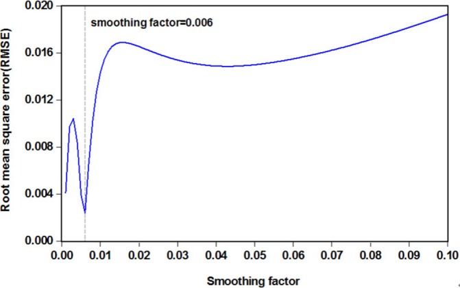
The RMSE values corresponding to different smoothing factors for the SARIMA-GRNN combined technique. It can be seen that when smoothing factor is 0.006, the lowest RMSE value is 0.0024. GRNN, generalised regression neural network; SARIMA, seasonal autoregressive integrated moving average.
Figure 4.
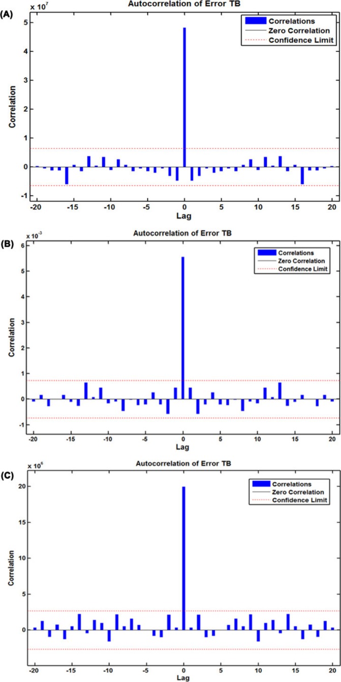
The resultant error autocorrelation function (ACF) plots for the three optimal hybrid models selected. (A) ACF plot of errors for the best-performing SARIMA-GRNN hybrid technique across varying lags; (B) ACF plot of errors for the best-performing SARIMA-NARNN hybrid technique across varying lags; (C) ACF plot of errors for the best-performing SARIMA-NARNNX hybrid technique across varying lags. GRNN, generalised regression neural network; NARNN, non-linear autoregressive neural network; NARNNX, non-linear autoregressive neural network with exogenous input; SARIMA, seasonal autoregressive integrated moving average; TB, tuberculosis.
The best-performing SARIMA-NARNN hybrid technique
To find the best-fitting NARNN model for the SARIMA error series, the hidden units and feedback delays ranged from 10 to 40 and 2 to 7, respectively, were iterated one by one. Ultimately, comprehensively taking all the performance indices into consideration, we identified the optimum model with 32 hidden neurons and 6 feedback delays. As presented in online supplementary figure S4, the preferred NARNN model had the minimum MSE value for training (0.003), validation (0.010) and testing (0.018), and it had the maximum R values for training, validation, testing subsets and for the entire dataset (0.882, 0.888, 0.619 and 0.823, respectively) (online supplementary figure S7). Moreover, the ACF plot of the residuals produced by the NARNN model revealed that all autocorrelations were within the estimated confidence intervals except for the one at the zero lag that should occur, suggesting that the errors behave like a white noise series (figure 4B). The Ljung-Box Q-test was associated with a large p value that also indicated that there did not seem to be autocorrelations remaining in the residuals (table 1). The response plot of the output elements for the randomly selected training, validation and testing subsets suggested that the preferred NARNN model can simulate the epidemic behaviours in the three grouped datasets due to the small errors that were located between approximately −0.2 and 0.2 (figure 5A). Additionally, the LM test demonstrated that the ARCH effects in the TB case notifications series were largely ameliorated in the residuals in the SARIMA-NARNN hybrid model (table 2). Therefore, the derived hybrid model is suitable for the current data. Next, the estimated results from the optimal hybrid approach were converted into the mimic and predictive values of the original observations using an inverse transform operation, as shown in table 3.
Figure 5.
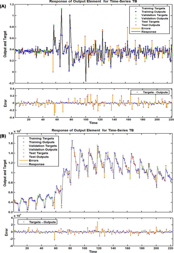
The corresponding time series response plots of outputs and targets for the best-undertaking SARIMA-NARNN and SARIMA-NARNNX hybrid models at various time points. (A) Response plot of the outputs and targets for the best-undertaking SARIMA-NARNN hybrid model; (B) Response plot of the outputs and targets for the best-undertaking SARIMA-NARNNX hybrid model. NARNN, non-linear autoregressive neural network; NARNNX, non-linear autoregressive neural network with exogenous input; SARIMA, seasonal autoregressive integrated moving average; TB, tuberculosis.
The best-performing SARIMA-NARNNX combined technique
To deeply mine the linear and non-linear patterns included in the TB incidence series, the preferred SARIMA-NARNNX hybrid model was built by trial and error. Finally, the SARIMA-NARNNX model with 17 hidden neurons and 4 feedback delays was determined to be the best-fitting model based on the minimum MSE for the training subset (18907817.559), the validation subset (19921017.940) and the testing subset (36872592.071), as well as with the maximum R values of the training, validation testing datasets and the entire dataset (0.994, 0.982, 0.986 and 0.992, respectively) (online supplementary figure S8). The ACF plot of errors from the optimal hybrid model showed no individually evident autocorrelations at varying lags except for the one at the zero lag, which are seeming satisfactory results with a white noise behaviour (figure 4C), the Ljung-Box Q-test further confirmed that this combined approach did not suffer from correlated residuals (table 1). The response plot of the output elements for the randomly selected training, validation and testing subsets indicated that the optimal technique can track the dynamic structure of the TB incidence series well (figure 5B). Importantly, the LM test showed that the volatility in the actual observations was essentially eliminated from the residuals of the best-fitting SARIMA-NARNNX hybrid model (table 2). All these results imply that the established model is appropriate and can be used to forecast future epidemic patterns of TB in mainland China (table 3).
Performance comparison
As shown in table 4, the MAE, MER, MAPE and RMSE values were the smallest in the SARIMA-NARNNX combined approach in the fitting stage and estimated stage. Among these four hybrid models, the curves mimicked and forecasted by the SARIMA-NARNNX hybrid model provided a better approximation to the actual data than the other models did (figure 6). As observed from the four measures, our proposed SARIMA-NARNNX hybrid model visibly lowered the model simulating and forecasting errors. Hence, this combined method should be adopted in the upcoming years for forecasting TB incidence. Moreover, to further test the performance superiority in the long-term prediction of TB incidence, we provided additional modelling and forecasting using the notified TB incidence, in which the data from January 1997 to December 2012 were used as the training set, and the data from January 2013 to March 2018 were used as the testing set. Online supplementary tables S3 and S4 and figures S9–S12 summarise the analytical results. Despite the degradation in its performance percentages, the proposed hybrid model can still be applied to perform long-term TB incidence predictions. In view of its superiority, this data-driven hybrid approach was thus remodelled on the whole dataset between January 1997 and March 2018 to predict the future long-trajectory trends of TB incidence (online supplementary table S5 and figures S13–S15). As shown in figure 7, the TB incident cases will continue the downward trend in the forecasted periods of April 2018 through December 2025 with a yearly reduction of approximately 3.002%.
Table 4.
Comparison of in-sample fitting and out-of-sample predicting performances among the best-performing approaches chosen
| Models | Simulating power | Predictive power | ||||||
| MAE | MER | MAPE | RMSE | MAE | MER | MAPE | RMSE | |
| SARIMA | 5636.303 | 0.062 | 0.067 | 8781.186 | 5726.262 | 0.061 | 0.060 | 7104.34 |
| SARIMA-GRNN | 4437.958 | 0.049 | 0.054 | 6939.078 | 5415.985 | 0.058 | 0.059 | 6155.964 |
| SARIMA-NARNN | 3283.274 | 0.035 | 0.043 | 5265.82 | 5259.556 | 0.056 | 0.055 | 6418.445 |
| SARIMA-NARNNX | 2878.484 | 0.031 | 0.038 | 4468.578 | 3563.179 | 0.038 | 0.038 | 4917.829 |
| Percentage reductions (%) | ||||||||
| D versus A | 48.930 | 50.000 | 43.284 | 49.112 | 37.775 | 37.705 | 36.667 | 30.777 |
| D versus B | 27.668 | 29.032 | 23.881 | 28.134 | 32.356 | 32.787 | 35.000 | 17.428 |
| D versus C | 7.182 | 6.452 | 7.463 | 9.079 | 29.625 | 29.508 | 28.333 | 21.123 |
GRNN, generalised regression neural network; MAPE, mean absolute percentage error; MER, mean error rate; MAE, mean absolute error; NARNN, non-linear autoregressive neural network; NARNNX, non-linear autoregressive neural network with exogenous input; RMSE, root mean square error; SARIMA, seasonal autoregressive integrated moving average.
Figure 6.
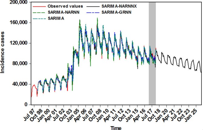
The comparison graph of the fitting and forecasting results among various models. GRNN, generalised regression neural network; NARNN, non-linear autoregressive neural network; NARNNX, non-linear autoregressive neural network with exogenous input; SARIMA, seasonal autoregressive integrated moving average.
Figure 7.
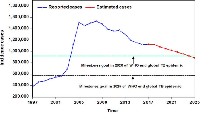
The comparison graph between the estimated epidemic trends of TB incidence from 2018 to 2025 and the milestones goals suggested by WHO. TB, tuberculosis.
A refers to the SARIMA model; B stands for the SARIMA-GRNN hybrid model; C signifies the SARIMA-NARNN hybrid model; D represents the SARIMA-NARNNX the hybrid model.
Discussion
As one of the oldest infectious diseases, many countries have been fighting TB for years, but TB is still by far one of the foremost public health problems in China and worldwide.9 Understanding the epidemic patterns of TB may facilitate the resolution of this issue. This is the first work to construct a hybrid technique (SARIMA-NARNNX) that combines a SARIMA model and a NARNN model with a time variable to forecast TB incidence, which may offer the base data and theoretical support to build and assess the control measures of TB. We compared the results derived from this data-driven method with the most widely used SARIMA model and the best-performing SARIMA-GRNN and SARIMA-NARNN combined approaches in the domain of epidemiological predictions. This SARIMA-NARNNX hybrid technique significantly outperforms the single SARIMA model, as well as the traditional SARIMA-GRNN and SARIMA-NARNN combined methods in both the simulating facet and the forecasting facet. Using this hybrid model, the performance-improvement percentages from the MAE, MER, MAPE and RMSE evaluation indices over the basic SARIMA method are 48.930%, 50.000%, 43.284% and 49.112%, respectively, in the training set and 37.775%, 37.705%, 36.667% and 30.777%, respectively, in the testing set. From these indices, the simulation and prediction errors are reduced using this hybrid method compared with the best-performing SARIMA-GRNN and SARIMA-NARNN combined approaches. In a similar fashion, we also adopted the basic NARNN method, along with the ETS approach to model TB incidence data; the ETS approach was recently shown to be a fairly effective tool for simulating incidence time series of infectious diseases (online supplementary figures S16–S19 and online supplementary tables S6 and S7).11 23 Likewise, the SARIMA-NARNNX technique is the best-performing method based on the aforementioned four measures (online supplementary table S8). Furthermore, in the present study, we observed that the SARIMA-NARNNX hybrid approach perfectly models and predicts the TB incidence data based on the MAPE measure, which is generally regarded as a useful index to judge the accuracy of a forecast. In terms of predictive ability, when the MAPE value is less than 5%, the forecast model is considered perfect. A model with a MAPE value falling within (5%, 10%) is considered highly accurate; a model with a MAPE value lying within (10%, 20%) is considered good; a model with MAPE value falling within (20%, 50%) is considered reasonable; and a model with a MAPE value greater than 50% is considered inaccurate.24 The trends fitted and predicted by the hybrid model show a very similar fluctuation pattern to the actual data (figure 6). In our experiments, all these results confirm that the SARIMA-NARNNX hybrid model is mechanically more robust and accurate and can better reflect internal regularities and track the future trends of TB incidence than the other methods. In addition, although the fitting and prediction accuracies of the other three models were lower than our proposed hybrid model, in terms of the modelling indices,24 the SARIMA, SARIMA-GRNN and SARIMA-NARNN models still do well in the prediction of TB notified cases, and the combined techniques of SARIMA-GRNN and SARIMA-NARNN give a better performance over the SARIMA method. In general, among these two combined approaches (SARIMA-GRNN and SARIMA-NARNN), the latter is superior to the former. This finding is fully aligned with previous studies concerning predictions for communicable diseases.9 14 19 The developed SARIMA-NARNNX hybrid model can serve as an effective tool for identifying the future trends of TB incidence in mainland China, and we also provide evidence that the time variable is conducive and instrumental in increasing the prediction accuracy. This parameter fails to be neglected when a disease displays notable seasonality and cyclicity. In this regard, our combined model seems to be appropriate for estimating the TB morbidity in other settings. However, it is worthwhile to note that, with the rapid development of data mining technology, much work is still needed to develop more accurate and precise techniques for evaluating and analysing the notified TB cases in mainland China.
It is well accepted that the accurate identification of seasonality plays a major role in timely responses and reasonably allocated resources for TB epidemics.3 In our present research, TB infection can occur during all seasons, but a clear seasonality with a periodicity of 12 months was noted with the aid of the HP technique from January 1997 to March 2018, and there was a peak in March and April of every year. Similar findings have already been verified in previous studies with the SARIMA-GRNN model, which was also constructed by using the nationally reported TB reported cases.3 7 At present, the seasonal variation of TB incidence has been observed in other countries or regions across the world.25 26 The evidence from a prior review containing 12 reports demonstrated that high-risk seasonality prevailingly occurred in the spring and summer.25 Two peaks of TB notifications were found in the Eastern Cape and in northern India, where the first stronger peak mainly spanned from April to June, and the weaker peak was annually observed from October to December.15 27 In China, a variety of complicated factors appear to be responsible for the TB incidence peak in the early spring, with the following reasons being of especial concern. The environment is gradually being destroyed by air pollution in China, and China has been under growing pressure, as PM2.5, PM10, NO2 and SO2, the key indicators of air pollution, increasingly hits new records in the winter in almost all the large cities. Importantly, few studies have revealed a positive correlation between air pollution and the seasonal risk of TB, and the potential hazards of air pollution on health exhibit an obvious lagged effect.28–31 In addition, the climatic characteristics of winter with low temperature and airflow compel people to conduct most social activities indoors, which may contribute to TB transmission due to poor ventilation and overcrowding.7 15 Perhaps the primary reason for the peak in the early spring is that the Lunar New Year, the most important annual festival in China, generally falls in the winter. This festival is associated with the largest annual population movement across the country by different means of transportation. In consideration of the length of the TB latent period, this festival effect may be a contributory factor in TB transmission.3 7 In addition, the other possible reasons for the risk seasonality of TB entail further investigation.
By characterising the TB notified cases in mainland China, a slight downturn since 2006 has been noted. Moreover, China has been on track to achieve the goal of reducing TB morbidity and mortality rates by 50% in 2015 relative to 1990.32 However, with the initiation of the ambitious goal to end TB around the world, WHO has proposed milestones targets for the TB incidence rate, mortality rate and incidents for 2020, 2025 and 2030 relative to 2015, along with the final elimination goal in 2035.10 Whether the targets can be achieved is still unknown, but our additional test results also support long-term projections of TB incidence. Hence, the SARIMA-NARNNX hybrid approach was rebuilt based on all the observations to understand the epidemiological situation in advance of the coming years. The results indicate that the TB incidence rate has already reached the target of less than 85 cases per 100 000 population before 202010 and the morbidity cases will continue to drop by a yearly average percentage of 3.002%. However, as presented in figure 7, the number of new cases may be far from the milestone targets by 2020 and 2025, and the expected cases of TB remain comparatively high, meaning that China will be still under the threat of TB for a long time. Therefore, to achieve the target of ending TB worldwide, more attention on further strengthening the comprehensive intervention strategies and proactively exploring new effective prophylactic methods for TB is expected (eg, the introduction of new vaccines, advanced diagnostic techniques and therapeutic techniques; comanagement of TB comorbidities; and the actualisation of universal health coverage and social protection).
In this work, we concentrate on the epidemic trend analysis of TB incidence and have succeeded in developing and assessing a hybrid technique with a potential for forecasting the long-term TB incidence data in mainland China. Moreover, the important findings drawn from this work are based on a sufficiently large TB incidence dataset spanning 29 years and a comprehensive comparison of models that are, currently, either the most extensively adopted or the most efficient for predicting infectious diseases incidence data. Nonetheless, several limitations still need to be considered. First, there is a lack of standardised methods that can be employed to identify the best-performing configuration and key parameters of ANNs; in applications, repeated attempts are required. Second, the underestimation of the total number of monthly incident cases is inevitable in passive contagious disease reporting systems as a result of a mixture of under-reporting of detected cases and underdiagnosis (eg, individuals may fail to access healthcare or they may fail to be diagnosed when they do). Third, weekly data may allow a greater examination of the temporal differences between years. Nevertheless, we do not perform further analysis due to the lack of available data. Fourth, the model was established without taking other drivers related to TB occurrence and development into consideration in addition to the case numbers and months. Fifth, this model should be regularly updated with new notified data to ensure its prediction accuracy. Lastly, this work is only focused on the TB incidence data forecasting in mainland China. Further studies involving predictions for various regions and different types of infectious diseases exhibiting marked seasonal and cyclic variations are required to verify the potential application of the SARIMA-NARNNX hybrid technique.
Conclusions
In summary, our proposed SARIMA-NARNNX method offers more accurate predictions for TB case notifications than that of the basic SARIMA, NARNN and ETS(M,A,A) methods, as well as the traditional SARIMA-GRNN and SARIMA-NARNN hybrid approaches. This model may be conducive and instrumental for government officials to rationally allocate health resources and appropriately formulate long-term preventive and control plans for TB. Additionally, the projected incidents display a potential slight downturn but still retain a fairly high morbidity level, so urgent action is needed to formulate additional comprehensive prevention, control and intervention strategies.
Supplementary Material
Acknowledgments
We thank all members involving the collection of TB data.
Footnotes
YW and CX contributed equally.
Contributors: YW, CX and JY conceived and proposed this work. SZ and ZW collected and analysed the data. LY and YZ improved the paper. All authors agreeed to submit this article.
Funding: This work was supported by the Graduate Student Innovation Fund of Hebei Province (no. CXZZBS2017130).
Competing interests: None declared.
Ethics approval: The ethical approval is not warranted for our present work as the monthly monitoring data of TB morbidity are publicly available in China.
Provenance and peer review: Not commissioned; externally peer reviewed.
Data sharing statement: All data were enclosed to the online supplementary materials.
Patient consent for publication: Not required.
References
- 1. Zhao Y, Li M, Yuan S. Analysis of transmission and control of tuberculosis in Mainland China, 2005-2016, based on the age-structure mathematical model. Int J Environ Res Public Health 2017;14:1192 10.3390/ijerph14101192 [DOI] [PMC free article] [PubMed] [Google Scholar]
- 2. WHO. Global tuberculosis report 2018. http://www.who.int/tb/publications/global_report/en/ (Accessed on 4 Dec 2018).
- 3. Cao S, Wang F, Tam W, et al. A hybrid seasonal prediction model for tuberculosis incidence in China. BMC Med Inform Decis Mak 2013;13:56 10.1186/1472-6947-13-56 [DOI] [PMC free article] [PubMed] [Google Scholar]
- 4. Murray CJ, Ortblad KF, Guinovart C, et al. Global, regional, and national incidence and mortality for HIV, tuberculosis, and malaria during 1990-2013: a systematic analysis for the Global Burden of Disease Study 2013. Lancet 2014;384:1005–70. 10.1016/S0140-6736(14)60844-8 [DOI] [PMC free article] [PubMed] [Google Scholar]
- 5. Moosazadeh M, Khanjani N, Nasehi M, et al. Predicting the Incidence of Smear Positive Tuberculosis Cases in Iran Using Time Series Analysis. Iran J Public Health 2015;44:1526–34. [PMC free article] [PubMed] [Google Scholar]
- 6. Pan HQ, Bele S, Feng Y, et al. Analysis of the economic burden of diagnosis and treatment of tuberculosis patients in rural China. Int J Tuberc Lung Dis 2013;17:1575–80. 10.5588/ijtld.13.0144 [DOI] [PubMed] [Google Scholar]
- 7. Wang H, Tian CW, Wang WM, et al. Time-series analysis of tuberculosis from 2005 to 2017 in China. Epidemiol Infect 2018;5. [DOI] [PMC free article] [PubMed] [Google Scholar]
- 8. Ade S, Békou W, Adjobimey M, et al. Tuberculosis case finding in Benin, 2000-2014 and beyond: a retrospective cohort and time series study. Tuberc Res Treat 2016;2016:1–9. 10.1155/2016/3205843 [DOI] [PMC free article] [PubMed] [Google Scholar]
- 9. Wang KW, Deng C, Li JP, et al. Hybrid methodology for tuberculosis incidence time-series forecasting based on ARIMA and a NAR neural network. Epidemiol Infect 2017;145:1118–29. 10.1017/S0950268816003216 [DOI] [PMC free article] [PubMed] [Google Scholar]
- 10. WHO. The end TB strategy. http://www.who.int/tb/strategy/en/ (Accessed on 19 May 2018).
- 11. Wang Y, Xu C, Zhang S, et al. Temporal trends analysis of human brucellosis incidence in mainland China from 2004 to 2018. Sci Rep 2018;8:15901 10.1038/s41598-018-33165-9 [DOI] [PMC free article] [PubMed] [Google Scholar]
- 12. Zhang X, Zhang T, Young AA, et al. Applications and comparisons of four time series models in epidemiological surveillance data. PLoS One 2014;9:e88075 10.1371/journal.pone.0088075 [DOI] [PMC free article] [PubMed] [Google Scholar]
- 13. He F, Hu ZJ, Zhang WC, et al. Construction and evaluation of two computational models for predicting the incidence of influenza in Nagasaki Prefecture, Japan. Sci Rep 2017;7:7192 10.1038/s41598-017-07475-3 [DOI] [PMC free article] [PubMed] [Google Scholar]
- 14. Zhou L, Yu L, Wang Y, et al. A hybrid model for predicting the prevalence of schistosomiasis in humans of Qianjiang City, China. PLoS One 2014;9:e104875 10.1371/journal.pone.0104875 [DOI] [PMC free article] [PubMed] [Google Scholar]
- 15. Azeez A, Obaromi D, Odeyemi A, et al. Seasonality and trend forecasting of tuberculosis prevalence data in eastern cape, south africa, using a hybrid model. Int J Environ Res Public Health 2016;13:757 10.3390/ijerph13080757 [DOI] [PMC free article] [PubMed] [Google Scholar]
- 16. Yan W, Xu Y, Yang X, et al. A hybrid model for short-term bacillary dysentery prediction in Yichang City, China. Jpn J Infect Dis 2010;63:264–70. [PubMed] [Google Scholar]
- 17. Zhang G, Huang S, Duan Q, et al. Application of a hybrid model for predicting the incidence of tuberculosis in Hubei, China. PLoS One 2013;8:e80969 10.1371/journal.pone.0080969 [DOI] [PMC free article] [PubMed] [Google Scholar]
- 18. Wei W, Jiang J, Gao L, et al. A new hybrid model using an autoregressive integrated moving average and a generalized regression neural network for the incidence of tuberculosis in heng county, China. Am J Trop Med Hyg 2017;97:799–805. 10.4269/ajtmh.16-0648 [DOI] [PMC free article] [PubMed] [Google Scholar]
- 19. Zhou L, Xia J, Yu L, et al. Using a hybrid model to forecast the prevalence of schistosomiasis in humans. Int J Environ Res Public Health 2016;13:355 10.3390/ijerph13040355 [DOI] [PMC free article] [PubMed] [Google Scholar]
- 20. Wu W, Guo J, An S, et al. Comparison of two hybrid models for forecasting the incidence of hemorrhagic fever with renal syndrome in Jiangsu Province, China. PLoS One 2015;10:e0135492 10.1371/journal.pone.0135492 [DOI] [PMC free article] [PubMed] [Google Scholar]
- 21. Wang Y, Xu C, Wang Z, et al. Seasonality and trend prediction of scarlet fever incidence in mainland China from 2004 to 2018 using a hybrid SARIMA-NARX model. PeerJ 2019;7:e6165 10.7717/peerj.6165 [DOI] [PMC free article] [PubMed] [Google Scholar]
- 22. Zhang X, Hou F, Li X, et al. Study of surveillance data for class B notifiable disease in China from 2005 to 2014. Int J Infect Dis 2016;48:7–13. 10.1016/j.ijid.2016.04.010 [DOI] [PMC free article] [PubMed] [Google Scholar]
- 23. Ke G, Hu Y, Huang X, et al. Epidemiological analysis of hemorrhagic fever with renal syndrome in China with the seasonal-trend decomposition method and the exponential smoothing model. Sci Rep 2016;6:39350 10.1038/srep39350 [DOI] [PMC free article] [PubMed] [Google Scholar]
- 24. Pao HT. Forecasting energy consumption in Taiwan using hybrid nonlinear models. Energy 2009;34:1438–46. 10.1016/j.energy.2009.04.026 [DOI] [Google Scholar]
- 25. Fares A. Seasonality of tuberculosis. J Glob Infect Dis 2011;3:46–55. 10.4103/0974-777X.77296 [DOI] [PMC free article] [PubMed] [Google Scholar]
- 26. Wubuli A, Li Y, Xue F, et al. Seasonality of active tuberculosis notification from 2005 to 2014 in Xinjiang, China. PLoS One 2017;12:e0180226 10.1371/journal.pone.0180226 [DOI] [PMC free article] [PubMed] [Google Scholar]
- 27. Thorpe LE, Frieden TR, Laserson KF, et al. Seasonality of tuberculosis in India: is it real and what does it tell us? Lancet 2004;364:1613–4. 10.1016/S0140-6736(04)17316-9 [DOI] [PubMed] [Google Scholar]
- 28. You S, Tong YW, Neoh KG, et al. On the association between outdoor PM2.5 concentration and the seasonality of tuberculosis for Beijing and Hong Kong. Environ Pollut 2016;218:1170–9. 10.1016/j.envpol.2016.08.071 [DOI] [PubMed] [Google Scholar]
- 29. Blount RJ, Pascopella L, Catanzaro DG, et al. Traffic-related air pollution and all-cause mortality during tuberculosis treatment in California. Environ Health Perspect 2017;125:097026 10.1289/EHP1699 [DOI] [PMC free article] [PubMed] [Google Scholar]
- 30. Smith GS, Van Den Eeden SK, Garcia C, et al. Air pollution and pulmonary tuberculosis: a nested case-control study among members of a northern california health plan. Environ Health Perspect 2016;124:761–8. 10.1289/ehp.1408166 [DOI] [PMC free article] [PubMed] [Google Scholar]
- 31. Lai TC, Chiang CY, Wu CF, et al. Ambient air pollution and risk of tuberculosis: a cohort study. Occup Environ Med 2016;73:56–61. 10.1136/oemed-2015-102995 [DOI] [PubMed] [Google Scholar]
- 32. Wang L, Zhang H, Ruan Y, et al. Tuberculosis prevalence in China, 1990-2010; a longitudinal analysis of national survey data. Lancet 2014;383:2057–64. 10.1016/S0140-6736(13)62639-2 [DOI] [PubMed] [Google Scholar]
Associated Data
This section collects any data citations, data availability statements, or supplementary materials included in this article.
Supplementary Materials
bmjopen-2018-024409supp001.pdf (819.3KB, pdf)