Age-structure and transient dynamics in epidemiological systems

Abstract

Mathematical models of childhood diseases date back to the early twentieth century. In several cases, models that make the simplifying assumption of homogeneous time-dependent transmission rates give good agreement with data in the absence of secular trends in population demography or transmission. The prime example is afforded by the dynamics of measles in industrialized countries in the pre-vaccine era. Accurate description of the transient dynamics following the introduction of routine vaccination has proved more challenging, however. This is true even in the case of measles which has a well-understood natural history and an effective vaccine that confers long-lasting protection against infection. Here, to shed light on the causes of this problem, we demonstrate that, while the dynamics of homogeneous and age-structured models can be qualitatively similar in the absence of vaccination, they diverge subsequent to vaccine roll-out. In particular, we show that immunization induces changes in transmission rates, which in turn reshapes the age distribution of infection prevalence, which effectively modulates the amplitude of seasonality in such systems. To examine this phenomenon empirically, we fit transmission models to measles notification data from London that span the introduction of the vaccine. We find that a simple age-structured model provides a much better fit to the data than does a homogeneous model, especially in the transition period from the pre-vaccine to the vaccine era. Thus, we propose that age structure and heterogeneities in contact rates are critical features needed to accurately capture transient dynamics in the presence of secular trends.

1. Introduction

The recurrent epidemics of immunizing infectious diseases, such as measles, mumps and rubella, represent well-documented examples of cyclic population dynamics [1–5], especially before the advent of routine infant immunization. Historically, such diseases mainly affected children owing to their extreme contagiousness and the long-lasting immunity elicited by infection. These characteristics, along with the direct mode of transmission of these diseases, mean that the epidemiological dynamics of many childhood diseases are capably modelled using the susceptible–exposed–infected–recovered (SEIR) model framework [6–9].

Early attempts to explain the determinants of these dynamics were initially focused on models that were not explicitly age-structured (e.g. [2,10–13]). We call these homogeneous models since ignoring age structure is equivalent to assuming homogeneous mixing, such that individuals from all age classes contact each other at the same rate. These models were able to reproduce the qualitative dynamics of some diseases by capturing key mechanisms: seasonal variation in contacts and susceptible depletion. However, following the classic work of Schenzle [14], Bolker & Grenfell [15] argued that quantitatively capturing pre-vaccine biennial cycles of measles required the explicit consideration of age-stratified pattern of contacts. The importance of age structure was subsequently called into question by Earn et al. [16], who demonstrated that the key ingredient necessary for a homogeneous model to successfully explain measles epidemics was the use of an appropriate seasonal forcing function (mimicking schools opening and closing), rather than age structure per se (see also [17]). These authors further demonstrated that, via a linear change of variables, a single bifurcation diagram may be constructed to summarize measles dynamics in response to changes in per capita birth rates or trends in vaccine uptake.

Models have been less successful at recreating dynamics during transition from the pre-vaccine to vaccine era of disease transmission. Under the assumption that the susceptible population is replenished by births and that a vaccine confers perfect protection against infection, theoretically, the vaccine era dynamics should be similar to the pre-vaccine era but with birth rates reduced to reflect the vaccine coverage reducing entry into the susceptible population, as predicted by Earn et al. [16]. However, a mathematical transmission–vaccination model that can capture key features of the observed transition from the regular pre-vaccine era measles epidemics to the more irregular vaccine era disease dynamics has remained elusive. While a homogeneous model with appropriately discounted susceptible influx rate can adequately reproduce the large decline in incidence after the introduction of vaccination, the transient dynamics accompanying the decline have been difficult to capture, in particular, features such as the changing periodicity [18].

In this paper, we compared the dynamics of a homogeneous model and an age-structured model of measles during the transition from the pre-vaccine to vaccine era. In the age-structured model, school-aged children were assumed to have high, seasonally varying contact rates (due to school-term forcing), while adult contact rates were lower and constant throughout the year. As in a homogeneous model, in the age-structured model, vaccination has the obvious effect of decreasing the fraction of the population susceptible to measles and hence a reduced mean transmission rate. However, age-structured contact rates lead to an additional effect of vaccination: reduced effective amplitude of seasonal forcing. This is due to the shift in transmission from primarily children to older age groups in which contact rates are less seasonal.

To illustrate the dynamical impact of age structure, we compared goodness of fit of a homogeneous model to that of a model with age structure, using historical measles data from London. In order to quantify the performance of models in explaining transient dynamics, we compared model fits for the pre-vaccine (1945–1968), pre-vaccine and early vaccine (1945–1978) and pre-vaccine to modern vaccine era (1945–1990). Our aim in this study was to examine the hypothesis that models that can capture the dynamic feedback between susceptible recruitment rates and the shifting age distribution of prevalence, together with the concomitant impact on the effective amplitude of seasonality will better explain the data. As a result, our models were deliberately simple and deterministic. We found that the age-structured model provided a better explanation of the data than the homogeneous model in both the pre-vaccine and the vaccination era.

Previous studies have recognized that age structure is an important component of the response of measles dynamics to vaccination [19–25]. In this paper, we emphasize that age structure is particularly relevant when there are secular trends in transmission, including the transition period soon after the start of routine immunization. We also provided empirical support for this claim by showing that age structure substantially improves the fit of a minimally complex model of measles vaccination to data. More broadly, our findings imply that age structure and heterogeneities in contact rates should be accounted for to capture transient dynamics associated with trends in the transmission of immunizing infectious diseases.

2. A transmission–vaccination model with an arbitrary number of age classes

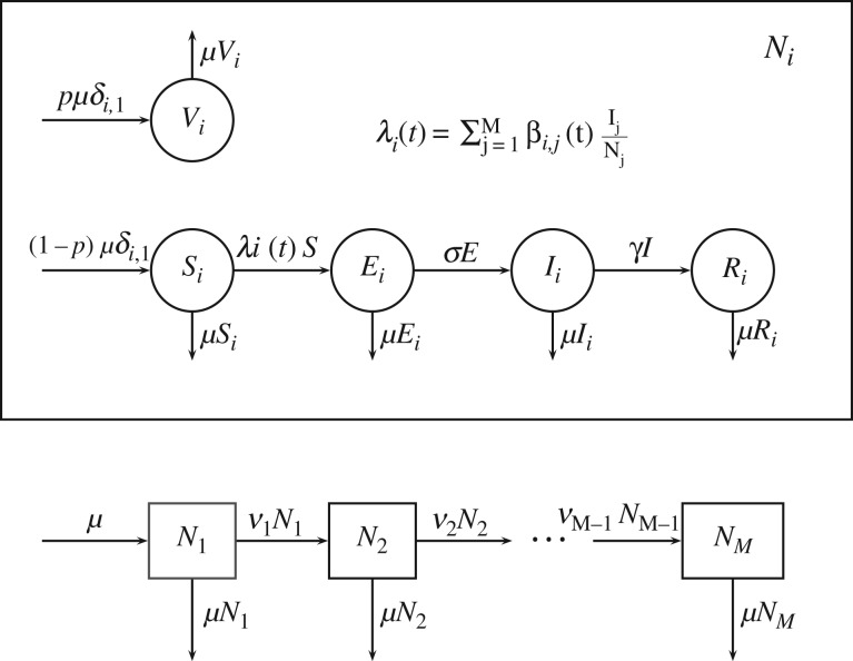
We considered a standard SEIR model, with an additional V component for individuals vaccinated at birth [9,26–28]. Each compartment was further divided into M age classes (M = 1 for the homogeneous model). For each age class i (i = 1 to M), we set N_i to be the total population of age class i and assume that this remains constant for all time t. Thus, V_i(t) + S_i(t) + E_i(t) + I_i(t) + R_i(t) = N_i for all t and we further assume that $N=\sum _{i=1}^M{N}_i=1$. The model is illustrated in figure 1 and the model equations are given in (2.1). The parameters of this model are described in table 1 and mathematical properties of this model are discussed in Magpantay [29].

Figure 1.

Schematic diagram of the age-structured compartmental model of vaccination used in §2–4.

Table 1.

Description of parameters of the general age-structured model.

symbol	parameter
M	number of age classes
μ	per capita birth and death rates
σ	incubation rate
γ	recovery rate
βi,j(t)	transmission rate between age class i and j. We assume βi,j(t) = βj,i(t) for all t, i and j
νi	ageing rate from age class i to i + 1, for $i=1,\dots ,M-1$. We also set ν0 = νM = 0
$\iota$	constant transmission rate from outside the population
p	fraction of newborns vaccinated
b	mean transmission rate among school-aged children, averaged over the entire year (refer to electronic supplementary material, S1)
s	amplitude of seasonality in the corrected term-time forcing function (refer to electronic supplementary material, S1)

For $i=1,\dots ,M$,

$$\begin{array}{rl}& \frac{\text{d}{V}_i}{\text{d}t}=p\mu {\delta }_{i,1}-\mu V_i+{\nu }_{i-1}{V}_{i-1}-{\nu }_i{V}_i,\\ & \frac{\text{d}{S}_i}{\text{d}t}=(1-p)\hspace{0.17em}\mu {\delta }_{i,1}-{\lambda }_i{S}_i-\mu S_i+{\nu }_{i-1}{S}_{i-1}-{\nu }_i{S}_i,\\ & \frac{\text{d}{E}_i}{\text{d}t}={\mathrm{\lambda }}_i{S}_i-\sigma E_i-\mu E_i+{\nu }_{i-1}{E}_{i-1}-{\nu }_i{E}_i,\\ & \frac{\text{d}{I}_i}{\text{d}t}=\sigma E_i-\gamma I_i-\mu I_i+{\nu }_{i-1}{I}_{i-1}-{\nu }_i{I}_i\\ \text{and}& \frac{\text{d}{R}_i}{\text{d}t}=\gamma I_i-\mu R_i+{\nu }_{i-1}{R}_{i-1}-{\nu }_i{R}_i.\end{array}\}$$ 2.1

Here, the subscript i refers to the ith age class, δ_i,j is the Kronecker delta function, ν_i is the ageing rate from age class i to i + 1 (ν₀ = ν_M = 0) and the force of infection experienced by the ith age class is given by

$${\mathrm{\lambda }}_i=\sum _{\hspace{0.17em}j=1}^M{\beta }_{i,j}(t)\frac{I_{\hspace{0.17em}j}}{N_{\hspace{0.17em}j}}+\iota .$$ 2.2

3. Average and effective transmission rates

To illustrate our claim that age-specific contact rates affect the overall dynamics of transmission, we define the average and effective transmission rate of the system of equations (2.1). For p ∈ (0, 1), let $V(t)=(1/\hspace{0.17em}p)\sum _{i=1}^M{V}_i(t)$, $S(t)=(1/(1-p))\sum _{i=1}^M{S}_i(t)$, $E(t)=(1/(1-p))\sum _{i=1}^M{E}_i(t)$, $I(t)=(1/(1-p))\sum _{i=1}^M{I}_i(t)$ and R(t) = $(1/(1-p))\sum _{i=1}^M{R}_i(t)$. Then from (2.1) we derive,

$$\begin{array}{rl}& \frac{\text{d}V}{\text{d}t}=\mu -\mu V,\\ & \frac{\text{d}S}{\text{d}t}=\mu -\mathrm{\lambda }S-\mu S,\\ & \frac{\text{d}E}{\text{d}t}=\mathrm{\lambda }S-\sigma E-\mu E,\\ & \frac{\text{d}I}{\text{d}t}=\sigma E-\gamma I-\mu I\\ \text{and}& \frac{\text{d}R}{\text{d}t}=\gamma I-\mu R.\end{array}\}$$ 3.1

Here, the force of transmission, λ, average transmission rate, $\overline{\beta }(t)$, and the effective transmission rate, $\hat{\beta }(t)$ (Earn, Rohani, Bolker & Grenfell 2000, unpublished results) are given by

$$\begin{array}{rl}\mathrm{\lambda }(t)=& \frac{\hat{\beta }(t)I(t)}{N}+\iota ,\hat{\beta }(t)=(1-p)\overline{\beta }(t)\text{and}\\ & \overline{\beta }(t)=\frac{\sum _{i,j=1}^M{\beta }_{i,j}(t)(I_{\hspace{0.17em}j}{S}_i/N_{\hspace{0.17em}j})}{\sum _{i,j=1}^M(I_{\hspace{0.17em}j}{S}_i/N)}.\end{array}\}$$ 3.2

The average transmission rate, $\overline{\beta }(t)$, reflects the transmission rate averaged over all contacts between susceptible and infected individuals in all age classes at a specific time t. The special case with homogeneous contact rates among age classes, β_i,j(t) = β_1,1(t) for all i and j, is equivalent to a homogeneous model with only one age class and the average transmission rate $\overline{\beta }(t)={\beta }_{1,1}(t)$.

The effective transmission rate, $\hat{\beta }(t)$, takes into account the reduction in transmission due to vaccination. For a homogeneous model, the system in (3.1) is equivalent to a homogeneous model with no vaccination but with the original transmission rate β_1,1(t) replaced everywhere by $\hat{\beta }(t)=(1-p){\beta }_{1,1}(t)$. This has been noted before by Earn et al. [16] for homogeneous models.

We note that we derived the expressions for the average and effective transmission rates under the assumption that the vaccine coverage p is constant. However, in this paper, we use the expressions in (3.2) to explore what happens to these transmission rates over long periods of time over which the vaccine coverage might have changed for a portion of that period.

In the model equations (2.1) and the derivation of the average and effective transmission rates above, we assumed that all age classes have the same constant death rate. The analysis is the same if we make the assumption that the death rate is zero in all age classes except for the last one.

4. Comparison of the dynamics of age-structured and homogeneous models

To illustrate the interplay between trends in transmission, seasonality and epidemiological dynamics, we contrasted the dynamics of an age-structured model (equations (2.1)) with two age classes (M = 2) with those of a homogeneous model (M = 1) before and after the introduction of vaccination. In both the homogeneous and age-structured cases, we assumed that contact rates were higher during school terms than school holidays such that β_1,1(t) = bT(t), where T(t) is the corrected term-time forcing function [9] and is fully described in the electronic supplementary material (electronic supplementary material, S1). In the age-structured model, the older age class is assumed to have lower and constant contact rates within its own age class and with the younger age class (${\beta }_{2,2}={\beta }_{1,2}={\beta }_{2,1}=\frac{1}{2}b$). All parameter values in the model were fixed except for b, the mean transmission rate and s, the amplitude of seasonality.

Numerical solutions of the homogeneous model identified stable periodic orbits with periods of 1, 2 and 3 years for different values of the mean transmission rate, b, and the amplitude of seasonality, s. Using numerical continuation techniques [30], we solved for periodic solutions of the model (with periods of 1, 2 or 3 years) at each point on a 400 × 200 grid over the (b, s) plane and determined the stability of these periodic solutions by calculating Floquet multipliers (refer to electronic supplementary material, S3).

To illustrate the dynamical impacts of immunization in an age-structure model, in figure 2a, we present an example trajectory of the model with two age classes as vaccine coverage jumps from zero to 30% in 1968 and linearly ramps up to 60% by 1980. These vaccine coverage values are motivated by estimates of measles immunization coverage in England and Wales from 1968 to 1980 [31]. In this section, vaccine coverage was maintained at 60% after 1980. This exercise provided us with some intuition on why the transition period is difficult to recreate in homogeneous models (as also shown in §5).

Figure 2.

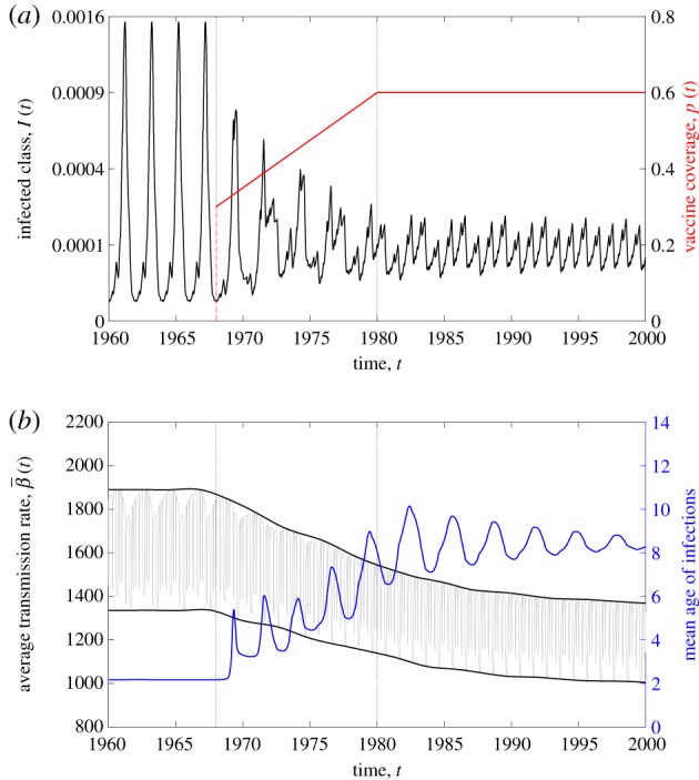
Dynamics of a model with two age classes (M = 2) after vaccination with $\mu =(1/50)\hspace{0.17em}{\text{yr}}^{-1}$, $\sigma =(365/8)\hspace{0.17em}{\text{yr}}^{-1}$, $\gamma =(365/5)\hspace{0.17em}{\text{yr}}^{-1}$, ν₁ = (1/12) yr⁻¹ and $\iota ={10}^{-4}\hspace{0.17em}{\text{yr}}^{-1}$. The younger age class N₁ is assumed to have higher and seasonal contact rates due to school-term forcing, β_1,1(t) = bT(t) where T(t) is the term-time forcing function [9]. The older age class N₂ is assumed to have contact rates given by β_2,2 = β_1,2 = β_2,1 = (1/2)b where $b=435\hspace{0.17em}{\text{yr}}^{-1}$. Refer to electronic supplementary material, S1 for further details on how these parameter values were chosen. (a) The aggregate prevalence (black) in a model with two age classes changes with vaccine uptake (red). A biennial cycle of epidemics is observed during the pre-vaccine era. The asymptotic dynamics in the vaccine era are annual. (b) The average transmission rate $\overline{\beta }(t)$ (black), its mean value and its amplitude of oscillation decreases with the increasing vaccine uptake given in (a). The mean age of the infected class (blue) increases with increasing vaccine uptake. (Online version in colour.)

Figure 2a demonstrates that biennial epidemics in the pre-vaccine era give way to longer period transients that eventually settle to annual epidemics [16,31]. The dynamical effects of increasing immunization coverage on the average transmission rate $\overline{\beta }(t)$ are shown in figure 2b. In this age-structured model, both the mean value of $\overline{\beta }(t)$ as well as the amplitude of seasonal variation decrease in the transition from pre-vaccine to vaccine era. As expected, the mean age of infection increases with increasing vaccine coverage. This shift in the age distribution of the infected class leads to a parallel shift in $\overline{\beta }(t)$ from high and strongly seasonal when the core transmission group is school-aged children (the first age group in our model), to lower and less seasonal when fewer children are infected.

In figure 3, we present the two-dimensional bifurcation diagram of the homogeneous model. The four different colours reflect the four distinct dynamical regimes investigated. In the white region, the system has a 1-year periodic solution that is stable, with no stable 2- or 3-year periodic solutions. In the light green region, stable 1-year and 2-year periodic solutions are observed, with asymptotic dynamics determined by the initial conditions of the model. In the orange region, the system has 1-year and 3-year stable periodic solutions, and, finally, in the dark green region, only a 2-year periodic solution was found to be stable.

Figure 3.

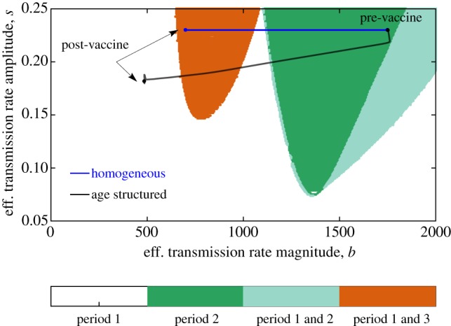
Bifurcation diagram of the homogeneous model over the mean transmission rate b and seasonality amplitude s. The blue line shows that under 60% vaccination, the homogeneous model is equivalent to a model with the same seasonality amplitude but a 60% lower transmission rate. By contrast, the two-age class model shifts to a lower seasonal amplitude and even lower mean transmission rate. Dynamics of a model with two age classes (M = 2) after vaccination using the same parameter values as in figure 2. (Online version in colour.)

We chose parameter values (b, s) = (b_hom, s_hom) for the homogeneous model that lie on the dark green region in the absence of immunization. As has been shown by Earn et al. [16] and demonstrated by equation (3.1) for the homogeneous model, vaccinating a fraction p of the population is equivalent to multiplying the mean transmission rate b by a factor of (1 − p). This does not affect the amplitude of seasonality s. Thus, before vaccination the homogeneous model has parameters b_hom and s = s_hom, and after vaccination with coverage p, the new model has dynamics that are equivalent to that of a homogeneous model with b = (1 − p)b_hom and s = s_hom. This is illustrated on the bifurcation diagram demonstrating that, in the vaccine era, the homogeneous model ends up in the orange region, with dynamics described either by an annual or triennial cycle.

We calculated the parameters (b, s) = (b_age, s_age) necessary for the age-structured model to have the same pre-vaccine era average transmission rate magnitude and amplitude as the homogeneous model. The details of this calculation are described in electronic supplementary material, S2. Notably, this results in a basic reproduction number (computed using the next-generation matrix method and using the mean transmission rate for the children’s age class) of about 7.8 for the age-structured model and about 24 for the homogeneous model. This discrepancy between the basic reproduction numbers between homogeneous and age-structured models displaying the similar prevalence has been documented before [21,32].

We confirmed that by using (b, s) = (b_age, s_age) the age-structured model displayed similar pre-vaccine era dynamics to the homogeneous model (a 2-year period with similar trajectory of the total number of infectious individuals). While the age-structured model does not have precisely the same bifurcation structure as a homogeneous model (discussed in electronic supplementary material, S4), we observed similar dynamics when their effective transmission rates $\hat{\beta }(t)$ had the same mean and amplitude. Thus, to illustrate how the dynamics of the age-structured model change under vaccination, we plotted the magnitude and amplitude of the effective transmission rate $\hat{\beta }(t)$ of the age-structured model on the bifurcation diagram in figure 3. Starting the age-structured model at the same point in the bifurcation diagram as the homogeneous model, we note that increasing vaccination leads to a divergence in their respective trajectories. In particular, late into the vaccine era, with steady vaccine coverage of p, the age-structured model ends up in the white region of the bifurcation diagram, with $\hat{\beta }(t)$ having magnitude less than (1 − p)b_hom and amplitude that is less than s_hom. This suggests that the vaccine era asymptotic dynamics of the age-structured model can only eventually settle down to a solution with a 1-year period. This clearly contrasts with the homogeneous model, which also allows for vaccine era dynamics with a stable 3-year period.

In figure 4, we present the asymptotic solutions of both homogeneous and age-structured models. In the pre-vaccine era, both display biennial cycles as shown in (figure 4a). After vaccination, we know that the homogeneous model can have either a 1-year or 3-year periodic solution, and the age-structured model has a 1-year periodic solution. The 3-year periodic solution of the homogeneous model and the 1-year periodic solution of the age-structured model are plotted together in figure 4b to show how the two models with similar pre-vaccine dynamics have very different vaccine era dynamics.

Figure 4.

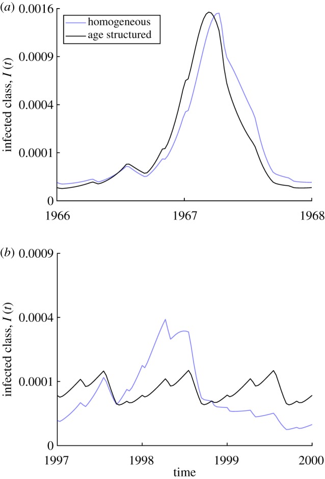
Comparison of the steady-state dynamics of a model with two age classes (M = 2) versus a homogeneous model (M = 1). Values used for the model are the same as in figure 2. (a) Pre-vaccine era, (b) vaccine era. (Online version in colour.)

5. Comparison of the fit of an age-structured and homogeneous model to London measles data (1945–1990)

To examine how the choice of model structure affects inferences made about data, we fitted a homogeneous model and an age-structured model with three age classes to historical reports of measles cases in London from 1945 to 1990. These models were based on (2.1) (with M = 3 for the age-structured case and M = 1 for the homogeneous case); full details are available in the electronic supplementary material, S4. All data and code required to reproduce the results of §5 are available via the Dryad Digital Repository (doi:10.5061/dryad.vj645q8). We emphasize that our goal here is not to produce the best performing model for measles, but to support our central thesis that age-structured models can better capture transient dynamics when trends in transmission exist.

Assuming a mean lifetime of 70 years, the first age class corresponded to ‘young children’ with a mean age of about 3.8 years (${\nu }_1=(1/4)\hspace{0.17em}{\text{yr}}^{-1}$). The next age class corresponded to ‘older children’ who are in school, with a mean age of about 14 years (${\nu }_2=(1/12)\hspace{0.17em}{\text{yr}}^{-1}$) and the last age class corresponded to ‘adults’. Details on computing these mean ages, the age distribution within each age class and other information about model fitting are provided in the electronic supplementary material, S4. We set β_2,2(t) to be a seasonal B-spline composed of six basis functions with an annual period. The other transmission rates are assumed to be constant over time: β_1,1(t) = β_YY, β_1,2(t) = β_2,1(t) = β_YC, β_1,3(t) = β_3,1(t) = β_YA, β_2,3(t) = β_3,2(t) = β_CA and β_3,3 = β_AA. In this notation for the transmission rates, the subscript Y refers to age class i = 1 (young children), C refers to age class i = 2 (older children) and A refers to age class i = 3 (adults). We also split the exposed and infectious compartments into three sub-compartments to allow for gamma-distributed latent and infectious periods [33,34].

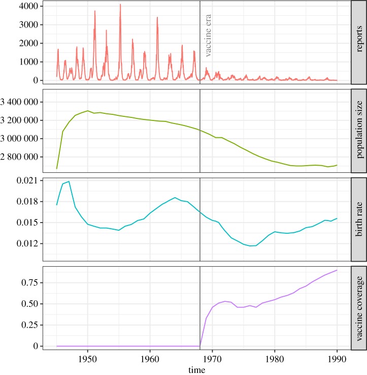
We obtained measles reports and demographic data (number of births and population sizes) for Greater London from Grenfell et al. [31]. We calculated the birth rates using the raw data, and estimated the population for inner London by multiplying the values for Greater London by 0.4 (refer to electronic supplementary material, S4). These covariates are plotted in figure 5. We see that the total population size N is changing over time. We set the birth rate in equations (2.1) to be a time-varying birth rate μ_B(t) using the data, and the ‘death’ rate in equations (2.1) to be a time-varying rate μ(t) that reflects both death and net migration, to keep the population size correct according to the data (refer to electronic supplementary material, S4).

Figure 5.

Measles notification data, population sizes, birth rates and vaccine coverage information for London from 1945 to 1990. (Online version in colour.)

The system of equations for the states of the model was deterministic (and hence the number of true cases over any interval is deterministic), but we modelled the reporting of cases using a negative-binomial distribution. We fitted the age-structured model to measles reports over three different periods: (1) 1945–1968, which represents the pre-vaccine period, (2) 1945–1978, which includes the first 10 years after the introduction of vaccination, and (3) 1945–1990, which extends deep into the vaccine era with high vaccine coverage (figure 5). For comparison, we also fitted a corresponding model with only one age class (M = 1) to data from these different eras. All parameter fitting was conducted using the trajectory matching function in the R package pomp [35].

A comparison of the Akaike information criterion (AIC) of the homogeneous (M = 1) and age-structured (M = 3) models at their maximum-likelihood parameter estimates is presented in table 2. This shows that the fit of the age-structured model is consistently much better than that of the homogeneous model, irrespective of the time period considered. The difference between the AICs of the two models is largest when they are fitted to the 1945–1978 data (pre-vaccine era to the early vaccine era). The best fit parameter values for the age-structured model are also presented in table 3.

Table 2.

Comparison of the homogeneous model and age-structured model (M = 3) at their maximum likelihood point estimates to different lengths of the London measles data. The homogeneous models each have 12 free parameters (including six spline coefficients for the seasonal transmission rate, one parameter for infection from outside the population, two parameters for the reporting model, three free initial conditions). The age-structured models have nine more parameters than the homogeneous models (including five additional transmission rate parameters and four additional initial conditions). Refer to electronic supplementary material, S4 for details.

length of data	log-likelihood of homogeneous model	log-likelihood of age-structured model	difference in log-likelihood	difference in AIC
1945–1968	− 7628	− 7497	131	− 244
1945–1978	− 10 754	− 10 531	223	− 428
1945–1990	− 13 793	− 13 638	155	− 292

Table 3.

Best fit parameter values of the age-structured model and 95% confidence intervals computed using profile likelihood. All transmission rates are in units of yr^{− 1}. The parameter $\iota$ in this model is the infection rate from outside the population in units of yr^{− 1} times the population size (refer to electronic supplementary material, S4.4). Due to the use of seasonal B-splines to fit the seasonal transmission rate for older children, the geometric mean of β_CC(t) over time at the maximum-likelihood point estimate is straightforward to compute and is presented here instead of the arithmetic mean. A summary of the descriptions of the model parameters is given in electronic supplementary material, tables S4.2–S4.3. Estimates of the basic reproduction number using the maximum-likelihood point estimates are provided in electronic supplementary material, S5.

length of data	parameter	max. likelihood estimate
1945–1968	βYY	39.5 (38.8, 40.0)
	βYC	4.2 (3.2, 4.8)
	βYA	1.8 (1.8, 2.8)
	βCA	52.8 (46.2, 60.3)
	geom. mean of βCC(t)	383.9
	βAA	154 (108, 246)
	$\iota$	3703 (3303, 5255)
	ρ	0.59 (0.57, 0.61)
	τ	0.56 (0.54, 0.58)
1945–1978	βYY	32.1 (22.5, 33.2)
	βYC	9.2 (6.0, 17.0)
	βYA	44.6 (15.2, 94.5)
	βCA	11.8 (7.6, 17.2)
	geom. mean of βCC(t)	417.9
	βAA	1199 (1109, 1267)
	$\iota$	10 110 (9659, 10 711)
	ρ	0.49 (0.48, 0.51)
	τ	0.65 (0.64, 0.67)
1945–1990	βYY	7.5 (6.4, 8.9)
	βYC	22.2 (20.0, 24.2)
	βYA	95.1 (83.5, 105.3)
	βCA	6.6 (3.2, 11.0)
	geom. mean of βCC(t)	359.6
	βAA	58.1 (16.0, 166.2)
	$\iota$	13 564 (12 963, 14 314)
	ρ	0.37 (0.36, 0.38)
	τ	0.72 (0.71, 0.74)

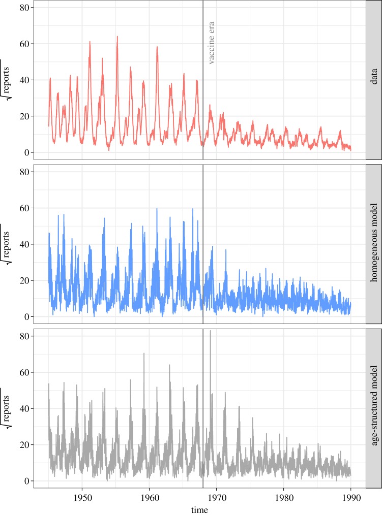
Representative realizations (including measurement noise) of the fitted age-structured and homogeneous models are shown in figure 6. This shows that both models can adequately reproduce the transition from annual cycles to the pronounced 2-year epidemics of measles in pre-vaccine London. Both models may still be lacking mechanisms to more accurately reproduce the vaccine era dynamics, but the results in table 2 show that the age-structured model does a better job than the homogeneous model. A comparison of the log-likelihood values corresponding to each data point of the homogeneous and age-structured models is also shown in figure 7.

Figure 6.

Weekly measles reports in London from 1945 to 1990 and representative simulations of the best fit age-structured and homogeneous models (using deterministic system of equations plus a negative-binomial reporting model). The number of reports are plotted using a square-root scale to allow for better comparison between the data and the simulations. (Online version in colour.)

Figure 7.

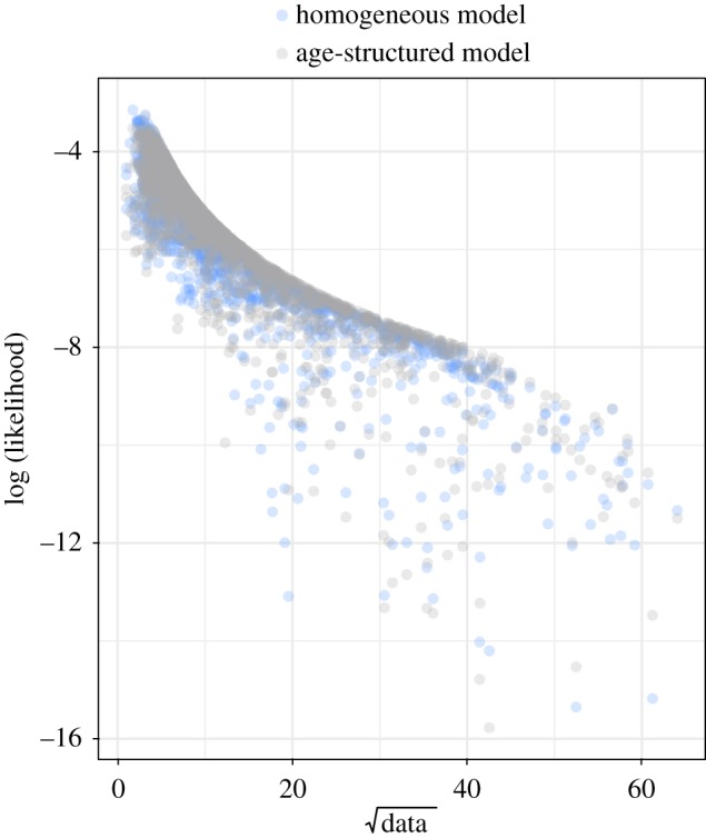
Comparison of the log-likelihoods corresponding to each data point (number of reported measles cases each week) for each model fitted to data from 1945 to 1990. We see from here that the age-structured model is better able to capture the intermediate values of the data than the homogeneous model when fitted to data from 1945 to 1990. This is still true when the models are fitted to just the pre-vaccine era data (1945–1968) and data from the pre-vaccine era to the early vaccine era (1945–1978). These are shown in electronic supplementary material, figure S4.10. The sum of all the likelihoods in these figures adds up to the likelihoods given in table 2. (Online version in colour.)

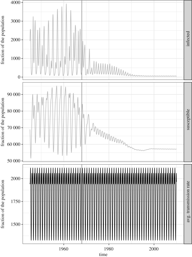
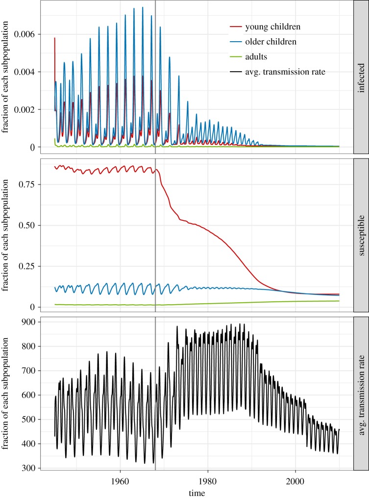
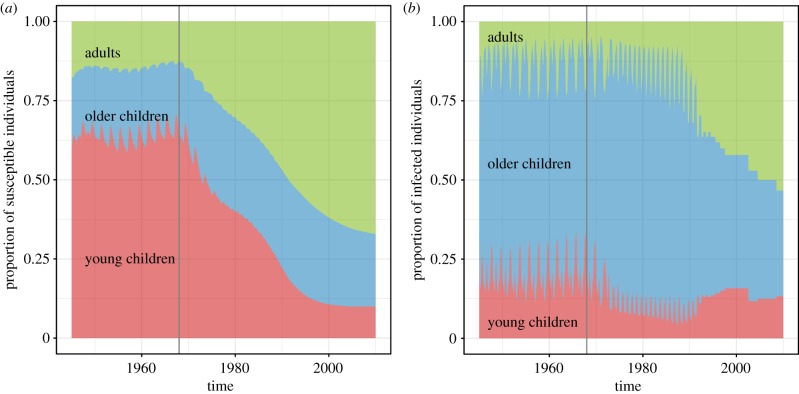
The trajectories of the infected and susceptible fractions of the two models as well as their average transmission rates ($\overline{\beta }(t)$, given by (3.2)) are shown in figures 8–9. In figure 8, the average size of the susceptible population in the homogeneous model is shown to not change very much relative to the entire population. The average transmission rate of the homogeneous model is also presented in the bottom panel to emphasize that this is not affected by vaccination. By contrast, in figure 9, the susceptibility of the young children in the age-structured model is shown to be markedly decreasing as more young children are vaccinated. This affects the average transmission rate of the model. In the bottom panel, we see that the average transmission rate of the age-structured model has an overall lower magnitude than that for the homogeneous model, and it changes with vaccination. It initially increases in magnitude during the transition period, then eventually decreases in magnitude and seasonality amplitude. The eventual decrease is similar to that displayed by the average transmission rate of the test model with two age classes shown in figure 2b; however, the temporary increase in magnitude during the transition period is not found in the test model with two age classes. This indicates that the transient dynamics during the transition period can be sensitive to the age structure of the model population. We present the changing composition of the infected and susceptible populations of the age-structured model in figure 10. As the number of infections from children go down, the fraction of the infected population that are adults increases. This is consistent with studies of age-stratified measles notification from England and Wales [23].

Figure 8.

The infected fraction, susceptible fraction and average transmission rate over time of the homogeneous model at its maximum-likelihood parameter values when fitted to the 1945–1990 data and simulated from 1945 to 2020. Recall that the average transmission rate $\overline{\beta }(t)$ from (3.2) is the transmission rate averaged over all contact between the different susceptible and infected age classes. With only one age class (M = 1) the average transmission rate simplifies to $\overline{\beta }(t)={\beta }_{1,1}(t)$ is the corrected school-term forcing function with a 1-year period that does not change from the pre-vaccine to the vaccine era.

Figure 9.

The infected fraction, susceptible fraction and average transmission rate over time of the age-structured model at its maximum-likelihood parameter values when fitted to the 1945–1990 data and simulated from 1945 to 2020. The infected and susceptible fractions of each of the three age classes are plotted. The average transmission rate $\overline{\beta }(t)$ changes over time as the age distributions of the infected and susceptible classes change (refer also to figure 10). Similar to figure 2b, $\overline{\beta }(t)$ has a high magnitude and amplitude of oscillation in the pre-vaccine era which is eventually replaced by a lower magnitude and amplitude in the late vaccine era. In the transition period, we actually observe a temporary increase in the magnitude of $\overline{\beta }(t)$ which we do not see in figure 2b. (Online version in colour.)

Figure 10.

The composition of the (a) susceptible and (b) infected populations changing over time in the age-structured measles model at its maximum-likelihood parameter values fitted to the 1945–1990 data and simulated from 1945 to 2020. The vertical line at 1968 indicates the start of the vaccine era. (Online version in colour.)

6. Discussion

In this paper, we used models of disease transmission based on the standard SEIR formalism to investigate the importance of age in the dynamics of infectious diseases in response to secular trends in transmission, resulting from, for example, sustained immunization. We found that when parametrized appropriately, the trajectories of the infectious classes generated using homogeneous and age-structured models can be very similar in the pre-vaccine era when most of the transmission may be occurring within one core group (usually school-aged children) with high and strongly seasonal contact rates. However, the dynamics of these models can diverge in the vaccine era, where the transmissions among school-aged children drastically go down and infections in older age classes, with lower mean contact rates and no seasonalilty, account for a significant fraction of transmission. The results in figure 3 show that vaccination in the age-structured model leads to a lower overall mean and amplitude of the effective transmission rate of the disease than does a homogeneous model. Both of these effects are due to the shift in disease transmission from primary school aged children to older age classes. Thus while an age-structured model can have similar dynamics to a homogeneous model in the pre-vaccine era, their predictions can be qualitatively different in the vaccine era (figure 4).

We have also shown that an age-structured model provides a much better fit (as quantified by AIC) to the London measles data compared to an analogous homogeneous model. As shown in table 2, this is true irrespective of the time period considered. The fact that the age-structured model fits the 1945–1968 (pre-vaccine era) data better than the homogeneous model suggests that age structure is already relevant even in the absence of vaccination. This difference in model performance may arise from changes in per capita birth rates during this period affecting the average transmission rate, as shown in figure 9 (and in electronic supplementary material, figure S4.7, which shows the changing transmission rates for the fit to the 1945–1968 data). The difference in the AIC of the age-structured and homogeneous models is largest when they are fitted to the 1945–1978 data, which encompasses 10 years of the early vaccine era. This result indicates a distinct advantage for age-structured over homogeneous models in explaining the transition period following the roll-out of the infant immunization programme. The difference between these models appears to be the most pronounced during this period because this is the interval over which the rate of change of the susceptible population’s age structure is most extreme. Finally, we found that a homogeneous model requires a much higher average transmission rate to model the 1945–1990 data compared to the age-structured model. This has important implications for control efforts and further supports our conclusion that age structure is an essential component for modelling pre-vaccine to vaccine era disease dynamics.

As in §4, the basic reproduction numbers of the age-structured models in §5 were found to smaller than those for homogeneous models fitted to the same data. These reproduction numbers, as well as the methods used to compute them are detailed in electronic supplementary material, S5. The estimated force of infection experienced by each age class is also shown in electronic supplementary material, S6. These results are compared to estimates of the force of infection and basic reproduction number in Edmunds et al. [21].

Our data fitting results support that the inclusion of age-structured contacts improves our models of transmission and vaccination. However, we note several ways in which the fit of our age-structured models might be improved. First, we expect that the use of stochastic models would be better for modelling measles epidemiology, especially during the vaccine era when incidence is lower so that intrinsic stochastic fluctuations assume greater dynamical importance (e.g. [32,36]). The deterministic models (both homogeneous and age structured) that we have fitted to the data currently require high levels of observation noise to compensate for the lack of stochasticity in the infection process. This is evident in figure 6. Second, we note that we have been using a linear interpolation of the annual national vaccine coverage data for the vaccine coverage function p(t) in the model. The use of this annual national average may not be best for modelling measles in London where the vaccine coverage in the city may differ from the national average. Since the dynamics of a model appear to be sensitive to our assumptions regarding vaccine coverage, we are currently looking at ways to improve our assumptions on the function p(t). In particular, we are investigating whether we can reduce this sensitivity by treating vaccine coverage as data, rather than as a precisely known covariate, using non-parametric approaches to represent the latent true vaccine coverage.

Finally, we note that as the demand for real-time forecasting of infectious disease dynamics increases, the need for mechanistic models that adequately translate the individual-level kinetics of transmission to their population-level impacts is clear.

Data accessibility

Data and code required to reproduce the results and figures in §5 are available via the Dryad Digital Repository (doi:10.5061/dryad.vj645q8).

Authors' contributions

All authors contributed to the development of the model, design of the study, analysis and interpretation of results. F.M.G.M. implemented the procedures and wrote the first draft of the paper. P.R. and A.A.K. edited and finalized the manuscript.

Competing interests

We declare we have no competing interests.

Funding

This work is supported by the Natural Sciences and Engineering Research Council of Canada, Queen’s University, the National Institutes of Health (grant no. R01AI101155) and by MIDAS, National Institute of General Medical Sciences (grant no. U54-GM111274).

References

- 1.Altizer S, Dobson A, Hosseini P, Hudson P, Pascual M, Rohani P. 2006. Seasonality and the dynamics of infectious diseases. Ecol. Lett. 9, 467–484. ( 10.1111/j.1461-0248.2005.00879.x) [DOI] [PubMed] [Google Scholar]
- 2.Anderson RM, May RM. 1982. Directly transmitted infections diseases: control by vaccination. Science 215, 1053–1060. ( 10.1126/science.7063839) [DOI] [PubMed] [Google Scholar]
- 3.Grassly NC, Fraser C. 2006. Seasonal infectious disease epidemiology. Proc. R. Soc. B 273, 2541–2550. ( 10.1098/rspb.2006.3604) [DOI] [PMC free article] [PubMed] [Google Scholar]
- 4.Metcalf CJE, Bjørnstad ON, Grenfell BT, Andreasen V. 2009. Seasonality and comparative dynamics of six childhood infections in pre-vaccination Copenhagen. Proc. R. Soc. B 276, 4111–4118. ( 10.1098/rspb.2009.1058) [DOI] [PMC free article] [PubMed] [Google Scholar]
- 5.Rohani P, Earn DJ, Grenfell BT. 1999. Opposite patterns of synchrony in sympatric disease metapopulations. Science 286, 968–971. ( 10.1126/science.286.5441.968) [DOI] [PubMed] [Google Scholar]
- 6.Anderson RM, May RM. 1991. Infectious diseases of humans. Oxford, UK: Oxford University Press. [Google Scholar]
- 7.He D, Ionides EL, King AA. 2010. Plug-and-play inference for disease dynamics: measles in large and small populations as a case study. J. R. Soc. Interface 7, 271–283. ( 10.1098/rsif.2009.0151) [DOI] [PMC free article] [PubMed] [Google Scholar]
- 8.Heesterbeek JAP, Diekmann O. 2000. Mathematical epidemiology of infectious diseases: model building, analysis and interpretation. Chichester, UK: John Wiley & Sons. [Google Scholar]
- 9.Keeling MJ, Rohani P. 2008. Modeling infectious diseases: in humans and animals. Princeton, NJ: Princeton University Press. [Google Scholar]
- 10.Hamer WH. 1906. Epidemic disease in England—the evidence of variability and of persistency of type. Lancet ii, 733–739. [Google Scholar]
- 11.London WP, Yorke JA. 1978. Recurrent outbreaks of measles, chickenpox and mumps. Am. J. Epidemiol. 99, 453–468. ( 10.1093/oxfordjournals.aje.a121575) [DOI] [PubMed] [Google Scholar]
- 12.Olsen LF, Schaffer WM. 1990. Chaos versus noisy periodicity: alternative hypotheses for childhood epidemics. Science 249, 499–504. ( 10.1126/science.2382131) [DOI] [PubMed] [Google Scholar]
- 13.Soper HE. 1929. The interpretation of periodicity in disease prevalence. J. R. Stat. Soc. 92, 34–73. ( 10.2307/2341437) [DOI] [Google Scholar]
- 14.Schenzle D. 1984. An age-structured model of pre- and post-vaccination measles transmission. IMA J. Math. Appl. Med. Biol. 1, 169–191. ( 10.1093/imammb/1.2.169) [DOI] [PubMed] [Google Scholar]
- 15.Bolker BM, Grenfell BT. 1993. Chaos and biological complexity in measles dynamics. Proc. R. Soc. Lond. B 251, 75–81. ( 10.1098/rspb.1993.0011) [DOI] [PubMed] [Google Scholar]
- 16.Earn DJD, Rohani P, Bolker BM, Grenfell BT. 2000. A simple model for complex dynamics transition in epidemics. Science 287, 667–670. ( 10.1126/science.287.5453.667) [DOI] [PubMed] [Google Scholar]
- 17.Finkenstädt BF, Grenfell BT. 2000. Time series modelling of childhood diseases: a dynamical systems approach. Appl. Stat. 49, 187–205. ( 10.1111/1467-9876.00187) [DOI] [Google Scholar]
- 18.Grenfell BT, Bjørnstad O, Finkenstädt BF. 2002. Dynamics of measles epidemics: scaling noise, determinism and predictability with the TSIR model. Ecol. Monogr. 72, 185–202. ( 10.1890/0012-9615(2002)072[0185:DOMESN]2.0.CO;2) [DOI] [Google Scholar]
- 19.Babad HR, Nokes DJ, Gay NJ, Miller E, Morgan-Capner P, Anderson RM. 1995. Predicting the impact of measles vaccination in England and Wales: model validation and analysis of policy options. Epidemiol. Infect. 1114, 319–344. ( 10.1017/S0950268800057976) [DOI] [PMC free article] [PubMed] [Google Scholar]
- 20.Bhattarchayya S, Ferrari MJ. 2016. Age-specific mixing generates transient outbreak risk following critical-level vaccination. Epidemiol. Infect. 145, 12–22. ( 10.1017/S0950268816002016) [DOI] [PMC free article] [PubMed] [Google Scholar]
- 21.Edmunds WJ, Gay NJ, Kretzschmar M, Pebody RG, Wachmann H, ESEN Project. European Sero-epidemiology Network. 2000. The pre-vaccination epidemiology of measles, mumps and rubella in Europe: implications for modelling studies. Epidemiol. Infect. 125, 635–650. ( 10.1017/s0950268800004672) [DOI] [PMC free article] [PubMed] [Google Scholar]
- 22.Ferrari MJ, Grenfell BT, Strebel PM. 2013. Think globally, act locally: the role of local demographics and vaccination coverage in the dynamic response of measles infection to control. Phil. Trans. R. Soc. B 368, 20120141 ( 10.1098/rstb.2012.0141) [DOI] [PMC free article] [PubMed] [Google Scholar]
- 23.Gay NJ, Hesketh LM, Morgan-Capner P, Miller E. 1995. Interpretation of serological surveillance data for measles using mathematical models: implications for vaccine strategy. Epidemiol. Infect. 115, 139–156. ( 10.1017/S0950268800058209) [DOI] [PMC free article] [PubMed] [Google Scholar]
- 24.Prada JM, Metcalf CJE, Takahashi S, Lessler J, Tatem AJ, Ferrari M. 2017. Demographics, epidemiology and the impact of vaccination campaigns in a measles-free world—can elimination be maintained? Vaccine 35, 1488–1493. ( 10.1016/j.vaccine.2017.02.008) [DOI] [PMC free article] [PubMed] [Google Scholar]
- 25.Trentini F, Poletti P, Merler S, Melegaro A. 2017. Measles immunity gaps and the progress towards elimination: a multi-country modelling analysis. Lancet Infect. Dis. 17, 1013–1014. ( 10.1016/S1473-3099(17)30421-8) [DOI] [PubMed] [Google Scholar]
- 26.Brauer F, van den Driessche P, Wu J. 2008. Mathematical epidemiology. Lecture Notes in Mathematics Berlin, Germany: Springer. [Google Scholar]
- 27.Kermack WO, McKendrick AG. 1927. A contribution to the mathematical theory of epidemics. Proc. R. Soc. 115A, 700–721. ( 10.1098/rspa.1927.0118) [DOI] [PubMed] [Google Scholar]
- 28.Scherer A, McLean A. 2002. Mathematical models of vaccination. Brit. Med. Bull. 62, 187–199. ( 10.1093/bmb/62.1.187) [DOI] [PubMed] [Google Scholar]
- 29.Magpantay FMG. 2017. Vaccine impact in homogeneous and age-structured models. J. Math. Biol. 75, 1591–1617. ( 10.1007/s00285-017-1126-5) [DOI] [PMC free article] [PubMed] [Google Scholar]
- 30.Kuznetsov YA. 1998. Elements of applied bifurcation theory, 2nd ed Berlin, Germany: Springer. [Google Scholar]
- 31.Grenfell B, Bjørnstad O, Kappey J. 2001. Travelling waves and spatial hierarchies in measles epidemics. Nature 414, 716–723. ( 10.1038/414716a) [DOI] [PubMed] [Google Scholar]
- 32.Magpantay FMG, Domenech de Cellès M, Rohani P, King AA. 2016. Pertussis immunity and epidemiology: mode and duration of vaccine-induced immunity. Parasitology 143, 835–849. ( 10.1017/S0031182015000979) [DOI] [PMC free article] [PubMed] [Google Scholar]
- 33.Lloyd AL. 2001. Realistic distributions of infectious periods in epidemic models: changing patterns of persistence and dynamics. Theor. Popul. Biol. 60, 59–71. ( 10.1006/tpbi.2001.1525) [DOI] [PubMed] [Google Scholar]
- 34.Wearing HJ, Rohani P, Keeling MJ. 2005. Appropriate models for the management of infectious diseases. PLoS Med. 2, 621–627. ( 10.1371/journal.pmed.0020320) [DOI] [PMC free article] [PubMed] [Google Scholar]
- 35.King AA. et al. 2015. pomp: Statistical Inference for Partially Observed Markov Processes. URL http://pomp.r-forge.r-project.org. R package, version 0.69-1.
- 36.Domenech de Celles M, Magpantay FMG, King AA, Rohani P. 2018. The impact of past vaccination coverage and immunity on pertussis resurgence. Sci. Transl. Med. 10, eaaj1748 ( 10.1126/scitranslmed.aaj1748) [DOI] [PMC free article] [PubMed] [Google Scholar]
Associated Data
This section collects any data citations, data availability statements, or supplementary materials included in this article.
Supplementary Materials
Data Availability Statement