Learning from scanners: Bias reduction and feature correction in radiomics

Highlights

• •Typically encountered CT exposure variations result in radiomics values distortion.
• •Proposed correction method suppresses the non-tumor related variation in radiomics.
• •The clinical relevance was shown using a 221 lung cancer patient cohort.

Abstract

Purpose

Radiomics are quantitative features extracted from medical images. Many radiomic features depend not only on tumor properties, but also on non-tumor related factors such as scanner signal-to-noise ratio (SNR), reconstruction kernel and other image acquisition settings. This causes undesirable value variations in the features and reduces the performance of prediction models. In this paper, we investigate whether we can use phantom measurements to characterize and correct for the scanner SNR dependence.

Methods

We used a phantom with 17 regions of interest (ROI) to investigate the influence of different SNR values. CT scans were acquired with 9 different exposure settings. We developed an additive correction model to reduce scanner SNR influence.

Results

Sixty-two of 92 radiomic features showed high variance due to the scanner SNR. Of these 62 features, 47 showed at least a factor 2 significant standard deviation reduction by using the additive correction model. We assessed the clinical relevance of radiomics instability by using a 221 NSCLC patient cohort measured with the same scanner.

Conclusions

Phantom measurements show that roughly two third of the radiomic features depend on the exposure setting of the scanner. The dependence can be modeled and corrected significantly reducing the variation in feature values with at least a factor of 2. More complex models will likely increase the correctability. Scanner SNR correction will result in more reliable radiomics predictions in NSCLC.

1. Introduction

Imaging is an essential part of the radiation oncology workflow: images are used for cancer staging and treatment planning and verification. Medical images contain a large amount of data, which enables their use in clinical practice to personalize radiation therapy for each patient [1]. The past five years have shown great improvement to automate clinical image processing by deriving quantitative features from these images, referred to as radiomics. Radiomics describe tumor phenotype using shape, statistical, and textural features extracted from images of different modalities: Computed Tomography (CT), Magnetic Resonance Imaging (MRI), Positron Emission Tomography (PET). Subsequently, machine learning algorithms use these radiomic features to predict patient survival time [2], [3], treatment toxicity [4], tumor habitat characterization [5].

Although the radiomics approach shows promising results, different feature definitions, image pre-processing methods, and imaging instruments make cross-institutional learning difficult [6], [7], [8], [9], [10]. The Image Biomarker Standardization Initiative (IBSI) standardized radiomics mathematical definitions and image pre-processing [11]. Still, imaging scanners are not designed for high quality radiomics, but for the best possible image quality for visual (human) interpretation. In daily practice, oncology institutions use their CT scanners with different imaging settings (reconstruction kernel, voxel spacing, X-ray tube exposure, etc) for each patient to optimize subsequent diagnosis and delineation. This lack of inter-scanner (scanner-to-scanner), intra-scanner (various settings within one scanner), and even test-retest (with exact the same settings) reproducibility makes the radiomics approach fragile [6], [7], [8], [9], [10]. The inter- and intra-scanner effects induce a non-tumor related variation in the measurements which can be described as bias in the radiomic features. Eventually, this bias may lead to misinterpretation of the radiomics data.

One of the main intra-scanner variations in the CT images is the X-ray tube exposure related to the scanner signal-to-noise ratio (SNR). In our study, we use phantom measurements to quantify how scanner SNR variation results in biasing the extracted features. We hypothesize that the SNR dependent bias can be characterized and quantified, providing the opportunity correct for it.

2. Materials and methods

2.1. Phantom

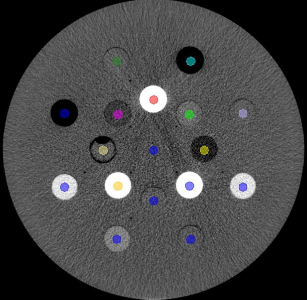
To investigate the influence of scanner SNR on radiomic features we used a commercial phantom (Gammex 467 CT phantom, Middletone, WI, USA). The phantom was used in the standard configuration with its 16 inserts of different tissue-like densities. We performed five sessions of scans with each 9 X-ray exposure settings (from 30 to 460 mAs) with a Brilliance Big Bore CT (Philips, Best, The Netherlands) using the Thorax protocol. The images were reconstructed with the B reconstruction kernel with pixel resolution 512 × 512. To extract radiomics, we delineated regions of interest (ROI) in all the 16 inserts and the phantom center (total of 17 ROIs) as equally-sized cylinders using the Pinnacle 16.0.2 treatment planning system (Philips Healthcare, Fitchburg, WI, USA). To avoid edge effects, we delineated the ROI smaller than the inserts as shown in Fig. 1. For radiomics extraction, we used open-source pyradiomics software with 25 HU binning and no re-sampling [12].

Fig. 1.

Gammex phantom configuration with cylindrical delineations. The 17 plug descriptions are in the supplementary A.

2.2. Patient cohort

To relate our phantom study to clinical applications, we used images of a 221 non-small cell lung cancer (NSCLC) cohort (supplementary Table B1) previously treated with (chemo)-radiotherapy and scanned with the same scanner as the phantom set. The data consists of radiotherapy treatment planning DICOM CT images with various scanner settings and physician-delineated primary NSCLC tumors as RT structure sets. The median X-ray tube exposure was 300 mAs. Radiomic features were extracted from the gross tumor volume (GTV) of the primary tumor with the same pyradiomics extraction settings as in the phantom set.

2.3. Correction method

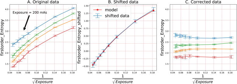
Using the five repeated measurements, we calculated mean and standard deviation for each exposure value and every ROI. We arbitrarily defined the target radiomic value (TRV) as the mean value of the radiomic feature measured with the 200 mAs exposure. The aim of the correction was to correct all exposure values to the value observed at 200 mAs as that was the median exposure value in the phantom set. Further data processing included: 1) TRV calculation (for 200 mAs) for each ROI in raw data (Fig. 2A), 2) Subtracting TRV from radiomic feature’s data, isolating the SNR trend in the data (Fig. 2B), 3) fitting the correction function (Fig. 2B), 4) Correcting the raw data (Fig. 2C).

Fig. 2.

Radiomics correction model in three steps: 1) shift original data to 0 with TRV, 2) fit the model using the shifted data, 3) correct the original data using the model.

As scanner SNR in CT images is inversely proportional to the square root of number of photons, and therefore, to $\frac{1}{\sqrt{\mathit{Exposure}}}$, we analyzed the relationships between radiomics values and $\frac{1}{\sqrt{\mathit{Exposure}}}$. To avoid overfitting, we trained a regression model with the only two predictors (excluding intercept): $\frac{1}{\sqrt{\mathit{Exposure}}}$ and ${\left(\frac{1}{\sqrt{\mathit{Exposure}}}\right)}^2$. We used no predictor scaling. Eventually, we defined the correction model as by formula (1), where w – model weights, b – intercept, E – exposure, Δ - correction factor. We developed the model using scikit-learn package for python, version 0.19.1 [13].

$$\begin{array}{c}R{F}_{\mathit{corrected}}=R{F}_{\mathit{measured}}+\mathrm{\Delta }\left(\mathrm{E}\right),\\ \mathrm{\Delta }\left(\mathrm{E}\right)=w_1\times \left(\frac{1}{\sqrt{E}}\right)+w_2\times {\left(\frac{1}{\sqrt{E}}\right)}^2+b.\end{array}$$ (1)

2.4. Radiomic feature correctability

We defined correctability as the ability to reduce scanner SNR influence on a radiomic feature. To assess correctability of a feature, we defined the correctability score (CS) as in formula (2). To derive the score, we used TRV-shifted data (Fig. 2B). The correctability score is a ratio: the numerator describes variability due to exposure (variance in means), the denominator describes intrinsic repeatability variance; $\mathrm{\Delta }RF$ stands for TRV-shifted radiomic feature values. For each exposure value in the range [30–460 mAs], numerator calculates mean and denominator calculates standard deviation of $\mathrm{\Delta }RF$ values. Then, numerator calculates standard deviation of means and denominator calculates mean standard deviation across the 9 exposure values. A value of 1 denotes that the correction is of the order of the noise and therefore is not very relevant. The correctability becomes more relevant at increasing values of CS. Eventually, the CS parameter is a measure of how correctable a feature is based on the phantom scans.

$$\mathit{CS}=\frac{std\left({\mathit{mean}}_{\mathit{while}\left\{exposure=EmAs\right\}}\left(\mathrm{\Delta }RF\right)\right)}{mean\left({\mathit{std}}_{\mathit{while}\left\{exposure=EmAs\right\}}\left(\mathrm{\Delta }RF\right)\right)}.$$ (2)

2.5. Correction evaluation

The final aim of the correction is to reduce the variance of the RF values due to the variation of noise, for this purpose, we defined the evaluation score (ES) as ratio of standard deviations before and after the correction calculated for each ROI and every radiomic feature (RF), where values above 1 indicate a gain of the correction mechanism, by formula (3):

$$ES\left(ROI\right)=\frac{StD\left(R{F}_{\mathit{before}correction}\right)}{StD\left(R{F}_{\mathit{after}correction}\right)}.$$ (3)

2.6. Clinical relevance of the phantom

Phantom radiomics studies should be applicable in clinical data. To assess clinical relevance, we evaluated 1) distribution overlap in features to test if a radiomic feature distribution in phantom set present absolute values of the same magnitude as values in clinical studies; 2) investigate how scanner SNR distorts feature values of clinical data by simulating (adding) noise to the scans.

When comparing distributions between the phantom and patient cohorts, note that all 17 phantom ROIs had the same shape in the phantom set, while in the patient cohort shape delineations differ between subjects [14]. Therefore, we performed the distribution comparison only for 4 vol-normalized features: ‘gldm DependenceNonUniformityNormalized’, ‘glrlm GrayLevelNonUniformityNormalized’, ‘glszm SizeZoneNonUniformityNormalized’, and ‘glrlm RunLengthNonUniformityNormalized’.

We cannot scan a patient with different exposure settings, therefore, we modeled scanner SNR in patient images by adding Poisson noise. The magnitudes of the Poisson noise were initially calibrated in phantom set to be adequate to real exposure settings (30–460 mAs) by applying Poisson noise of different magnitudes to the phantom images with the maximum exposure of 460 mAs (supplementary Fig. B3). As the next step, Poisson noise with the magnitude calibrated for −160 mAs SNR reduction was applied in patient images. We used those generated images to extract radiomics and evaluate the relative shift in features. The relative shift is defined in formula (4) and evaluates how large the difference between feature values in original ($R{F}_{\mathit{original}}$) and SNR-influenced ($R{F}_{-160\mathrm{m}\mathrm{A}\mathrm{s}}$) images is if compared to the interquartile range in the feature distribution ($\mathit{IQ}{R}_{0.75-0.25}(R{F}_{\mathit{original}})$):

$$\mathit{relative}shift({\mathit{patient}}_i,RF)=\left|\frac{R{\mathrm{F}}_{-160\mathrm{m}\mathrm{A}\mathrm{s},i}-R{F}_{\mathit{original},i}}{\mathit{IQ}{R}_{0.75-0.25}(R{F}_{\mathit{original}})}\right|\times 100\%.$$ (4)

3. Results

3.1. Radiomic feature correctability

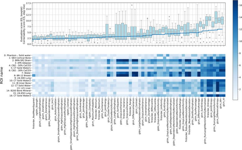
We calculated the correctability score (CS) for each radiomic feature – 92 scores in total. If the CS of a radiomic feature is close or less than one, the intrinsic reproducibility variance is equal to the scanner SNR-caused variation; that makes the feature uncorrectable. Therefore, we chose for the correctability threshold of CS > 2, meaning that the correctable scanner SNR variance is 2 times higher than the intrinsic reproducibility in a radiomic feature. Based on this threshold criterion, we selected 62 features for further analysis. The upper panel of Fig. 3 shows CS for each selected radiomic feature as the step blue line.

Fig. 3.

Correctability (2) and Evaluation (3) scores for the selected 62 radiomic features and 17 ROIs. The color bar represents the evaluation score (ES): the darker, the larger reduction in standard deviation was obtained.

3.2. Correction evaluation

To assess whether the exposure dependence could be corrected with our model we calculated the evaluation score (ES). All 62 selected with the CS > 2 threshold criterion radiomic features showed significant (ES versus 1 Wilcoxon signed-rank test p < 0.01) reduction in standard deviation (averaged across the ROIs) using our additive model. Forty-seven out of 62 radiomic features showed significant (ES versus 2 Wilcoxon test p < 0.05) at least 2 times standard deviation reduction. In summary, the upper panel boxplot (Fig. 3) describes ES distribution across 62 radiomic features and 17 ROIs.

We evaluated how different materials react on the scanner noise by calculating 17 ROIs’ ES for each radiomic feature and placed the scores in lower panel of Fig. 3. Interestingly, ROIs 9 and 15 (low density plugs, <−600 HU) have low correctability, on the other hand, ROIs 2 and 8 (28 and −45 HU mean density respectively) have good correctability. These results show that different materials react differently on scanner SNR in radiomic features: some materials are more dependent on scanner SNR than others are.

3.3. Clinical relevance of the phantom

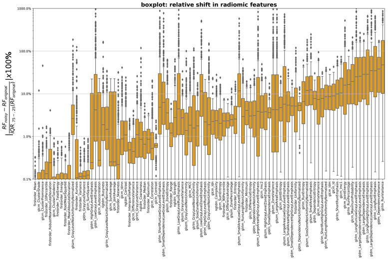
In our study, we used phantom measurements to simulate and characterize the acquisition of radiomic features for clinical scans. Fig. 4 shows how large the relative shift (4) in radiomic features is while applying Poisson noise of the magnitude equivalent of −160 mAs scanner SNR reduction. For example, relative shift of 10% means that −160 mAs reduction in a patient scan causes feature value to change 10% relative to the feature distribution width in the patient cohort.

Fig. 4.

Relative shift (4) in radiomic features (in ascending order) versus feature names while applying Poisson noise (equivalent to decreasing scanner SNR, mAs) in the images of the NSCLC cohort.

In addition, we evaluated overlap between the clinical and phantom sets in 4 normalized feature distributions (supplementary Fig. B1). We found that the distributions have clear overlap; therefore, phantom radiomics are at least partly relevant for clinical scans.

4. Discussion

We systematically investigated the dependence of radiomic feature values on scanner SNR using a commercial phantom and a patient cohort of lung cancer patients. The phantom measurements were obtained using a standard clinical protocol, where the SNR was varied by changing exposure settings from 30 to 460 mAs. We showed that many radiomic features form a trend with the scanner SNR, making the value of the feature not only dependent on the tumor, but also on a specific scanner setting. To remedy this effect, we developed a method to correct the radiomic features for scanner SNR.

4.1. Radiomics correctability

We used correctability score (CS) to separate radiomic features which are biased and correctable in terms of scanner SNR from those that are not. Although Spearman correlation is a reliable criterion for trend detection, it does not include the intrinsic repeatability of the measurement. For instance, the statistical radiomic feature ‘Energy’ (supplementary C) has a high Spearman correlation with scanner SNR, but the feature’s correctable trend variance is smaller than its intrinsic repeatability making correction not effective. Therefore, we defined CS that assesses both intrinsic repeatability and correctable trend variance. Of the 92 features considered, 62 show a CS > 2, indicating that they have a dependence on scanner SNR that dominates the repeatability. Note that stability for different exposure settings (CS < 1) does not mean a radiomic feature is stable for other scanner settings (image reconstruction kernel, voxel spacing, etc).

4.2. Correction model

Given that there is a trend of the feature value with exposure, we hypothesize that it is possible to correct for the variation. We chose an additive quadratic regression model and used X-ray tube exposure as the predictor. Adding more variables (e.g. uncorrected feature values and/or its intersection term with exposure) might benefit the correction for some features where additive terms cannot explain trends for different ROIs perfectly. For instance, for the feature ‘glrlm GreyLevelVariance’ (see supplementary C), the correction seems to depend on the density of the plug, suggesting that a model incorporating the exposure and the mean HU as predictors could improve the correction significantly. We did not pursue developing more complicated correction models in this paper since our main goal was give a proof of principle regarding correctability, and since other issues such as overfitting must be considered when making the model more complex. supplementary C shows the scanner SNR correction in all the 92 features.

4.3. Clinical relevance of the phantom and correction model

In using phantom measurements to study scanner dependence of clinical scans, it is paramount that the phantom (material) is representative for the patient case [8]. We compared the distribution of radiomic features in a clinical cohort with the distribution in a phantom. Ideally, the distribution of the features in both phantom and patient cohorts should be identical for all features. Firstly, as has been described before, a part of the ‘texture’ features are dependent on the shape or the size of the ROI [14]. Comparing the distribution of these is not relevant since we use artificial (cylindrical) regions, therefore only features insensitive to volume or shape could be used. Some typical examples of these features are given in the supplementary data (supplementary B). Overlap is present in for almost all features. This suggests that the properties of the phantom captured by the radiomic features are at least partly relevant for the patient cohort. Future work is needed to develop plugs that are identical to patient material, although a perfect match with the patient cohort for all features is unrealistic [8].

As a second method to test the applicability in the clinical situation, we simulated for each patient scan what the effect would have been if the scan was made with lower exposure. For this we applied Poisson noise to images, where the quantitative relation between the noise amplitude and the exposure was derived from the phantom scans. We found that scanner SNR results in change of the radiomics values for the clinical scans (Fig. 4). For a large part of the patients/features, a moderate change in the exposure resulted in more than 10% change of the radiomic feature compared to the width of the distribution of the whole cohort. When using the radiomic features as an input for a personalized outcome prediction, this will clearly affect the value of the prediction for individual patients.

Fave et al also investigated the effect of noise in patient CT’s on radiomic features by adding noise to the scans. Their findings is in line with ours, namely that the effect is significant, leading to the conclusion that scanning with a range of patient dose should be avoided [15]. Our finding is however in contrast with the conclusion of Mackin et al. [8]. Their measurements were done using the Credence Cartridge Radiomics phantom, and reached the conclusion that SNR of the scan was not likely to be of significant influence since for the rubber insert (which was taken to be most representative for tumor tissue) the effect of the changing tube current was small. Their argument is that the addition of the noise to the scan negligible due to the tumor inhomogeneity. However, the added noise simulations by Fave et al. and us show that for the patient scans involved (in both cases NSCLC patients) the noise indeed affects feature values significantly.

5. Conclusion

We found that 62 out of 92 radiomic features strongly depend on scanner SNR. Due to this dependence, non-tumor related variation is added to the features’ values, seriously limiting the use of radiomics in clinical applications. We showed that a simple additive model effectively corrects the undesired variation for 47 out of 62 features. By comparing a NSCLC cohort with the phantom set, we showed that variation in scanner SNR is a reality in a typical clinical cohort, and thus is an actual problem in using radiomics for prediction modeling and personalized medicine.

Funding statement

This work was supported by the Netherlands Organization for Scientific Research (NWO) [grant number P14-19].

Contributors

IZ – data acquisition, method development, analysis, and manuscript writing.

JB – clinical data acquisition, manuscript revision, and supervision of IZ.

AT, PK, and LW – reproducibility evaluation method development.

ZS – development of pyradiomics extension for DICOM.

AD – manuscript revision, and supervision of IZ.

RF – manuscript revision, and supervision of IZ.

RM – data acquisition, method development, manuscript writing and revision, and supervision of IZ.

All co-authors contributed to proof-reading of the manuscript.

Declaration of Competing Interest

Andre Dekker reports grants from Varian Medical Systems, personal fees from Medical Data Works BV, personal fees from UHN Toronto, personal fees from Hanarth Fund, personal fees from Johnson & Johnson, outside the submitted work; In addition, Andre Dekker has a patent Systems, methods and devices for analyzing quantitative information obtained from radiological images US Patent 9721340 B2 issued.

Appendix A. Supplementary data

The following are the Supplementary data to this article:

Data Availability

Radiomic feature table (phantom set) and Jupyter notebook for analysis are stored at: https://github.com/ivanzhovannik/radiomics_correction_CTSNR.

Phantom set (DICOM images) coupled with its RTSTRUCT file (delineations) are accessible at: https://xnat.bmia.nl/app/template/XDATScreen_report_xnat_projectData.vm/search_element/xnat:projectData/search_field/xnat:projectData.ID/search_value/stwstrategyps4.

References

- 1.Gillies R.J., Kinahan P.E., Hricak H. Radiomics: images are more than pictures, they are data. Radiology. 2016;278(2):563–577. doi: 10.1148/radiol.2015151169. [DOI] [PMC free article] [PubMed] [Google Scholar]
- 2.Aerts H.J. Decoding tumour phenotype by noninvasive imaging using a quantitative radiomics approach. Nat Commun. 2014;5:4006. doi: 10.1038/ncomms5006. [DOI] [PMC free article] [PubMed] [Google Scholar]
- 3.Hosny A. Deep learning for lung cancer prognostication: a retrospective multi-cohort radiomics study. PLoS Med. 2018;15(11) doi: 10.1371/journal.pmed.1002711. [DOI] [PMC free article] [PubMed] [Google Scholar]
- 4.Abdollahi H. Rectal wall MRI radiomics in prostate cancer patients: prediction of and correlation with early rectal toxicity. Int J Radiat Biol. 2018;94(9):829–837. doi: 10.1080/09553002.2018.1492756. [DOI] [PubMed] [Google Scholar]
- 5.Sala E. Unravelling tumour heterogeneity using next-generation imaging: radiomics, radiogenomics, and habitat imaging. Clin Radiol. 2017;72(1):3–10. doi: 10.1016/j.crad.2016.09.013. [DOI] [PMC free article] [PubMed] [Google Scholar]
- 6.Mackin D. Measuring computed tomography scanner variability of radiomics features. Invest Radiol. 2015;50(11):757–765. doi: 10.1097/RLI.0000000000000180. [DOI] [PMC free article] [PubMed] [Google Scholar]
- 7.Mackin D. Harmonizing the pixel size in retrospective computed tomography radiomics studies. PLoS ONE. 2017;12(9) doi: 10.1371/journal.pone.0178524. [DOI] [PMC free article] [PubMed] [Google Scholar]
- 8.Mackin D. Effect of tube current on computed tomography radiomic features. Sci Rep. 2018;8(1):2354. doi: 10.1038/s41598-018-20713-6. [DOI] [PMC free article] [PubMed] [Google Scholar]
- 9.Shafiq-Ul-Hassan M. Accounting for reconstruction kernel-induced variability in CT radiomic features using noise power spectra. J Med Imaging (Bellingham) 2018;5(1) doi: 10.1117/1.JMI.5.1.011013. [DOI] [PMC free article] [PubMed] [Google Scholar]
- 10.Shafiq-Ul-Hassan M. Intrinsic dependencies of CT radiomic features on voxel size and number of gray levels. Med Phys. 2017;44(3):1050–1062. doi: 10.1002/mp.12123. [DOI] [PMC free article] [PubMed] [Google Scholar]
- 11.Alex Zwanenburg, S.L., Martin Vallières, Steffen Löck, Image biomarker standardisation initiative. arXiv preprint arXiv:1612.07003, 2016.
- 12.van Griethuysen J.J.M. Computational radiomics system to decode the radiographic phenotype. Cancer Res. 2017;77(21):e104–e107. doi: 10.1158/0008-5472.CAN-17-0339. [DOI] [PMC free article] [PubMed] [Google Scholar]
- 13.Pedregosa F. Scikit-learn: machine learning in python. J Mach Learn Res. 2011;12:2825–2830. [Google Scholar]
- 14.Welch M.L. Vulnerabilities of radiomic signature development: the need for safeguards. Radiother Oncol. 2018 doi: 10.1016/j.radonc.2018.10.027. [DOI] [PubMed] [Google Scholar]
- 15.Fave X. Preliminary investigation into sources of uncertainty in quantitative imaging features. Comput Med Imaging Graph. 2015;44:54–61. doi: 10.1016/j.compmedimag.2015.04.006. [DOI] [PubMed] [Google Scholar]
Associated Data
This section collects any data citations, data availability statements, or supplementary materials included in this article.
Supplementary Materials
Data Availability Statement