An Improved Model for the Rate–Level Functions of Auditory-Nerve Fibers

Abstract

Acoustic information is conveyed to the brain by the spike patterns in auditory-nerve fibers (ANFs). In mammals, each ANF is excited via a single ribbon synapse in a single inner hair cell (IHC), and the spike patterns therefore also provide valuable information about those intriguing synapses. Here we reexamine and model a key property of ANFs, the dependence of their spike rates on the sound pressure level of acoustic stimuli (rate–level functions). We build upon the seminal model of Sachs and Abbas (1974), which provides good fits to experimental data but has limited utility for defining physiological mechanisms. We present an improved, physiologically plausible model according to which the spike rate follows a Hill equation and spontaneous activity and its experimentally observed tight correlation with ANF sensitivity are emergent properties. We apply it to 156 cat ANF rate–level functions using frequencies where the mechanics are linear and find that a single Hill coefficient of 3 can account for the population of functions. We also demonstrate a tight correspondence between ANF rate–level functions and the Ca²⁺ dependence of exocytosis from IHCs, and derive estimates of the effective intracellular Ca²⁺ concentrations at the individual active zones of IHCs. We argue that the Hill coefficient might reflect the intrinsic, biochemical Ca²⁺ cooperativity of the Ca²⁺ sensor involved in exocytosis from the IHC. The model also links ANF properties with properties of psychophysical absolute thresholds.

Introduction

All acoustic information relayed to the CNS is encoded in the spike patterns of auditory-nerve fibers (ANFs). A thorough understanding of ANF response properties is therefore crucial for understanding the auditory system as a whole. In mammals, each ANF is excited via a single ribbon synapse in a single receptor cell, the inner hair cell (IHC) (Liberman et al., 1990), and ANF responses therefore also provide insights into the operation of these intriguing synapses (for review, see Fuchs, 2005; Moser et al., 2006; Nouvian et al., 2006; Matthews and Fuchs, 2010).

A key feature of the responses of ANFs is the dependence of their spike rates on the amplitude [sound pressure level (SPL)] of auditory stimuli. Identification of the primary determinants of these rate–level functions would enable better understanding of the changes in them produced by, for example, acoustic trauma and hearing loss (Heinz and Young, 2004) and of related and clinically relevant perceptual phenomena.

Comprehensive models of the auditory periphery have been developed which, among other features, produce ANF rate–level functions similar to those observed experimentally (Zhang et al., 2001; Meddis, 2006). However, the sheer number of model parameters makes it difficult to identify those that are most relevant for producing a particular output and makes their fine-tuning to experimental data impossible. A more tractable and highly influential model was developed by Sachs and Abbas (1974). It consists of a mechanical stage, capturing the basilar membrane (BM) vibration amplitude as a function of the sound amplitude, followed by a “transducer” stage that describes the spike rate of an ANF as a function of BM displacement as a saturating power function. This model provides good fits to empirical rate–level functions of ANFs in mammals, birds, and reptiles (Yates et al., 1990; Eatock et al., 1991; Saunders et al., 2002), but has several limitations: it does not predict the correlation of spontaneous rate with ANF sensitivity observed in mammals and cannot account for spike rates lower than the spontaneous rate. Furthermore, the optimal value of the exponent in the model's transducer stage appears to vary systematically (between approximately 1 and 3) with spontaneous rate, implying different mechanisms at different synapses (Eatock et al., 1991). The model therefore has limited utility for identifying physiological mechanisms.

Here, we develop an improved model which overcomes these limitations. When this model is applied to our dataset, the optimal value of the exponent is 3, suggesting a common synaptic mechanism. We argue that this exponent might reflect the intrinsic cooperativity of the Ca²⁺ sensor involved in fast exocytosis from the IHC. If this were the case, it would link the rate–level functions to a key biochemical process in the IHC. Since the exponent is the same as that derived independently from perceptual data (Heil and Neubauer, 2003; Neubauer and Heil, 2004), our model also links ANF rate–level functions with psychophysics. A preliminary account of some of these data has been presented (Heil et al., 2010).

Materials and Methods

The data for this study were derived from a subset of the ANFs whose interspike interval distributions during spontaneous activity were analyzed and modeled by us previously (Heil et al., 2007). All surgical and recording procedures are described in detail by Heil et al. (2007) and are therefore only briefly summarized here. All procedures were approved by the Monash University Department of Psychology Animal Ethics Committee.

Surgery

Four adult cats (two females, two males; weighing 3–3.5 kg) with clean tympani were anesthetized with pentobarbitone sodium (40 mg/kg, i.p.) and prepared for recordings from the left auditory nerve. Anesthesia was maintained throughout the experiment by intravenous injections of pentobarbitone mixed with physiological saline containing 5% glucose. The electrocardiogram was continuously monitored, and rectal temperature was held at ∼38°C by a thermostatically controlled DC blanket.

Recording procedures

Single ANFs were recorded with micropipettes or glass-insulated tungsten microelectrodes with impedances of 4–7 MΩ at 1 kHz, with the cat in an electrically shielded, sound-attenuating room. The electrode was advanced in a dorsoposterior-to-ventroanterior and slightly medial-to-lateral direction, similar to the approach of Liberman and Kiang (1978). The nerve was contacted close to its exit from the internal auditory meatus to minimize the possibility of recording from the cochlear nucleus. The progressions of characteristic frequency (CF; the frequency to which an ANF is most sensitive) with depth of the electrode tip from the surface of the nerve were similar to those reported by Liberman and Kiang (1978, their Fig. 4A–E). The range and distribution of spontaneous rates also matched those reported previously for the cat (Liberman and Kiang, 1978), and the characteristics of the interspike interval distributions during spontaneous activity matched those of ANFs (Gaumond et al., 1982; Li and Young, 1993). Together, these observations indicate that we recorded from the auditory nerve and not the cochlear nucleus, and that we sampled fibers from most areas of the auditory nerve.

Figure 4.

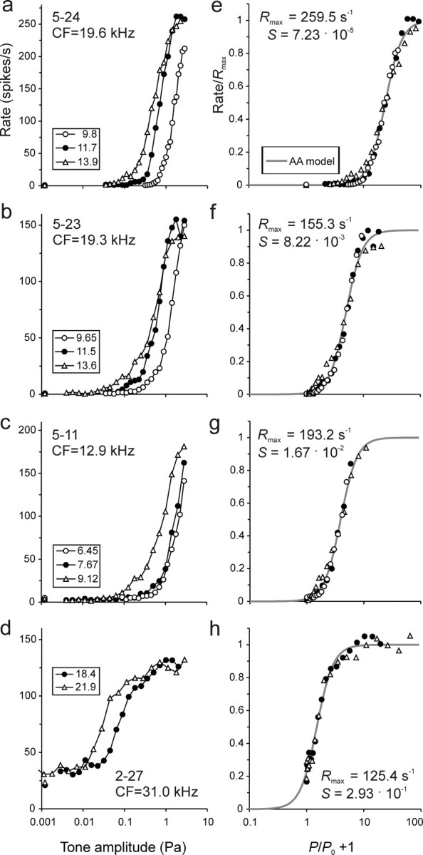
Representative rate–level functions and their fit with the AA model with β = 3. a–d, The 10 functions are from different ANFs and were selected to represent a wide range of CFs, stimulus frequencies, and spontaneous rates. The CF and stimulus frequency (F; in kilohertz) are identified. Symbols represent measured spike rates. The spontaneous rate is plotted near the ordinate, at an arbitrary abscissa value. Solid lines and dashes (for the spontaneous rate) represent the fits of each data set with the AA model with β = 3.

The electrode signal was amplified, filtered, and passed through a Schmitt trigger. Spike event times (defined as the time when the amplified and filtered electrode signal crossed the Schmitt-trigger level) were stored on disc with 1 μs resolution. Acoustic stimuli were digitally produced (Tucker-Davis Technologies) and presented to the cat's left ear via a calibrated sealed sound delivery system consisting of a STAX SRS-MK3 transducer in a coupler (Sokolich, 1981). Noise and tone bursts were used as search stimuli to increase the likelihood of detecting ANFs with very low spontaneous discharge rates. Once a fiber was encountered and well isolated, its CF was determined by manually varying the stimulus frequency and amplitude. Next, up to 200 repetitions of tones with a given frequency (initially at the CF) and duration and shaped with cosine-squared rise and fall times were presented at a fixed rate, at SPLs increasing from low to high values in small steps. This protocol was followed by recording the ANFs' spontaneous activity for a period of at least 12.5 s. If the recording conditions were still stable, another tone stimulus was selected and the protocol repeated. Most commonly, the new stimulus had a frequency of 1, 0.75, 0.5, or 0.25 octaves below the CF. Here, we report only data obtained with tone frequencies of at least 0.5 octaves below the CF, tone durations of 100 ms, rise and fall times of 4.2 ms, and a presentation rate of 4 Hz. Given the results of Saunders et al. (2002), it is unlikely that the rate–level functions and estimated model parameters would have been very different had we presented the tones of different SPLs in a random fashion rather than in ascending order.

Data analysis

All computations and model fitting were performed in Excel 2000 using the Newton procedure of the Solver module.

Response measure

In agreement with the common practice in the literature, we counted all spikes elicited during the tone duration and over all repetitions and computed a mean spike rate from this number. We chose to slightly prolong the analysis window, by 10 ms, beyond the end of the tone bursts to compensate for delays in the ANF responses, which can amount to a few milliseconds, particularly in ANFs of low CF and low spontaneous rate (Heil and Neubauer, 2001). The measure of mean spike rate ignores the fact that the rate is not constant during the tone's duration but adapts. However, the characteristics of adaptation, such as the time constants, do not seem to vary systematically with SPL (Chimento and Schreiner, 1991). Similarly, adaptation does not greatly affect the shape of the rate–level function (Smith and Brachman, 1980; Yates et al., 1990; Winter et al., 1990), and spike rate measures taken from different time spans after tone onset, or obtained with different tone durations, simply result in rate–level functions that are scaled versions of one another (Sachs and Abbas, 1974; Smith, 1977; Winter et al., 1990). Thus, it seems justified to neglect adaptation at this stage of modeling. The spontaneous rate was computed from all spikes occurring during the silent interval of at least 12.5 s at the end of each recording protocol.

Model fitting

Competitive curve fitting.

We needed to compare the well-established Sachs and Abbas (1974) model with the new model proposed here [termed the rate–additivity (RA) and amplitude–additivity (AA) models, respectively; see Results]. The two models were fitted to each data set using two variants of a multistep competitive curve fitting (CCF) procedure, which ensured that the Solver would converge on the best solution possible with each model. The CCF procedure works as follows. In one variant, a given data set was first fitted with the RA model using a multistep procedure as described below. Then the AA model was fitted, but initially to the RA model function obtained from the previous step rather than to the data. The parameters obtained from this approximation were then used as the starting parameters to fit the AA model again, but now to the data. In an analogous way, the RA model was then fitted again, using the parameters from the first fit of the RA model as the starting parameters. Again, the fit of the RA model was first to the AA model function obtained from the previous step, and the parameters obtained from this approximation were then used as the starting parameters to fit the RA model again, now to the data, but only if the starting condition was better than the results obtained from the first round fit of the RA model. Otherwise, those parameters were taken. In this way, it was assured that the fits could only improve (or remain the same) from one round to the next. This alternation continued until both models had been fitted three times to a given data set. In the second variant, the CCF procedure started with the AA model and proceeded analogously. The better fit of each model across these two CCF variants was then selected.

Starting values of model parameters.

The starting values of the four parameters of each model (see Results) for the first round of the CCF procedure were selected based on the data to be fitted. The starting value for the parameter capturing the maximum rate, R_max, in either model was 1.1 times the maximum spike rate observed in the data set; that for the parameter capturing the spontaneous rate, R_spont, in either model was 0.9 times the minimum spike rate observed. In the AA model, the starting value for P₀ was determined indirectly via an estimate of R_spont (Eqs. 5–11). The starting values for the sensitivity parameter, K_RA and K_AA in the RA and AA models, respectively, were derived from an estimate of the point of inflection, taken as the tone amplitude where the observed (interpolated) spike rate was halfway between its minimum and its maximum. The starting value of the exponent α in the RA model was set to the value most commonly used in the literature, 2, while that of the exponent β in the AA model was set to 3, the value that provided the best fit across the population in initial exploratory fits. However, the CCF procedure was robust against changes in the starting values of α and β.

Multistep fitting procedure.

Each of the two sets of six rounds of the CCF procedure consisted of four successive fitting steps. In the first step, only parameters K_RA and R_spont for the RA model and K_AA and P₀ for the AA model were allowed to vary. In the second step, R_max was also a free parameter, and in the final two steps all four parameters were allowed to vary. In fits of the data, where α and β were fixed (see Results), all steps were run with α and β fixed.

Choice of cost functions.

We minimized two different cost functions: (1) the sum of the squared differences of spike rates between data and model and (2) the sum of the squared differences of the logarithms of the spike rates between data and model. The first, linear cost function is that most commonly used in the literature. The second, logarithmic cost function minimizes the relative rather than the absolute errors. Particularly in fibers with low spontaneous rates and at low to medium SPLs, the variance of the number of spikes per tone was approximately equal to the mean number of spikes per tone (a Poisson process predicts equality), as has been observed previously (Teich and Khanna, 1985). Consequently, a given difference in spike rates of, for example, 5 spikes per second between model and data constitutes a significant error when the expected rate is low, say, 1 spike per second, but a nonsignificant error when the expected rate is high, say, 200 spikes per second. These considerations argue for minimizing the relative error. However, when no spikes were elicited by any of the repetitions of a particular stimulus, usually low-amplitude tones, or when no spike occurred spontaneously, these response measures, although valid, had to be excluded from the logarithmic fits, since the logarithm of zero is undefined. This exclusion not only reduces the reliability of the fit, but introduces systematic bias. Also, after exploring the issue of heteroscedasticity in detail, it became obvious that the results obtained with the linear cost function were superior. We therefore focus on the results obtained with the linear cost function, but note that the results obtained with the logarithmic cost function were similar. We explored the issue of heteroscedasticity by first computing the (linear and logarithmic) differences between each fitted model and the data. For each rate–level function, these differences were computed not only for the actual SPLs tested and for the spontaneous activity, but also for SPLs in between, for 101 SPLs (supporting points) altogether. For this purpose, the spontaneous rate was assigned an SPL below that of the lowest SPL used, at a distance matching the spacing between tested levels. The 101 supporting points were then equally spaced between the SPL assigned to the spontaneous rate and the highest SPL used for a given rate–level function. The differences between model and data at these supporting points were obtained by interpolation, either on a linear or a logarithmic rate axis, and then squared. These squared differences were then averaged across all 156 rate–level functions at corresponding supporting points. These averaged squared differences fluctuated along the level axis, peaking at the 21 points corresponding to the tested SPLs. With the linear cost function, the amplitude of these fluctuations increased slightly with increasing SPL, as expected, while with the logarithmic cost function, it decreased with increasing SPL. With the logarithmic cost function, the amplitude of the fluctuations at low SPLs was much larger than that of those at the high SPLs with the linear cost function, probably as an unavoidable consequence of the discrete nature of the ultimate response measure (spike counts) and its pronounced relative changes when the counts are low (a single spike more can double the response rate estimate). To quantify the heteroscedasticity, we averaged the squared differences obtained from the 50 low-SPL supporting points (Δ_low²), those obtained from the 50 high-SPL supporting points (Δ_high²), and those obtained from all 101 supporting points (Δ_all²). The measure of heteroscedasticity, H, was then calculated as follows:

The ratio of these measures for the linear and the logarithmic fits was smaller than 1 (H_lin/H_log was ∼0.54 for the RA model and ∼0.65 for the AA model), thus favoring the linear fits.

To compare the quality of the fits across different rate–level functions, which may have been based on different numbers of rate–level combinations (n; usually 21 but in some cases fewer than that), and model variants with different numbers of free parameters (n_fp; either 3 or 4), we calculated a deviation measure D, which takes this into account and which is defined as follows:

Here, Δ is the difference between the empirical spike rate and that predicted (or between their logarithms), and n is the number of data points. The lower the value of D, the better the fit.

Results

In the following, we first present the Sachs and Abbas (1974) model and our new model and then evaluate them on real data. Several functions generated with both models are illustrated in Figure 1. A focus will lie on the exponent in the new model and the questions of whether a single value suffices to account for all ANF rate–level functions and how this value links to known physiological and biochemical processes in the IHC.

Figure 1.

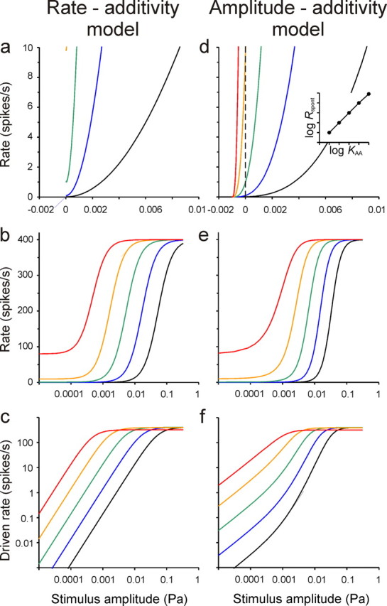
Hypothetical rate–level functions generated according to the RA model (left) and the new AA model (right). For the RA model, the five functions were generated according to Equation 3 with a common R_max = R_{max d} + R_spont = 400 spikes per second and common α = 2. The sensitivity K_RA differs by one order of magnitude between neighboring functions, thus increasing from the black to the red function by four orders of magnitude. R_spont is set to covary over nearly four orders of magnitude, from 0.01 to 80 spikes per second, to reproduce the empirical correlation between sensitivity and spontaneous rate. For the AA model, the five functions were generated according to Equation 5 with a common R_max = 400 spikes per second, β = 3, and P₀ = 1 mPa. Only the sensitivity parameter K_AA increases from the black to the red function over four orders of magnitude. a, d, Functions with rate and amplitude plotted on linear axes and providing a high resolution of low rates and low amplitudes. In a, only the three functions with the lower values of R_spont are visible. In d, the vertical dashed line marks P = 0, and the intersections of the functions with that line allow the resulting values of the spontaneous activity, R_spont, to be read off; R_spont varies over nearly four orders of magnitude and in nearly direct proportion to the sensitivity K_AA (inset). b, e, Full changes in rate plotted against stimulus amplitude on the conventional logarithmic axis (covering a 100 dB range). c, f, Growth of the driven component of the rate, i.e., of R_d(P) = R(P) − R_spont, with stimulus amplitude in double-logarithmic coordinates. With the RA model (c), the steepest slopes are essentially identical to the value of α, independent of spontaneous rate, whereas for the AA model (f), the steepest slopes are less than the value of β, the more so the higher the spontaneous rate.

The Sachs–Abbas or rate–additivity model

The model proposed by Sachs and Abbas (1974) comprises a mechanical stage, essentially capturing the BM mechanics as a function of the stimulus amplitude, followed by a saturating nonlinearity, termed the “transducer” stage by Sachs and Abbas (1974). This transducer stage describes the spike rate of an ANF as a function of the BM displacement. At frequencies around the fiber's CF, BM displacement grows in a nonlinear (“compressive”) manner with stimulus amplitude (for review, see Robles and Ruggero, 2001; Hudspeth, 2008), and at least two model parameters are required to describe this function. Here, we consider only responses to frequencies well below the CF, where BM displacement can be well approximated as a linear function of stimulus amplitude P (in pascals) (Robles and Ruggero, 2001). This avoids the complications of BM nonlinearities, simplifies the model considerably, and reduces the number of model parameters from six to four. In essence, the model reduces to its transducer stage. Sachs and Abbas (1974) further assumed that the total firing rate R(P) of an ANF can be expressed as the sum of the stimulus-driven rate R_d(P) and a spontaneous rate R_spont; we will therefore refer to it as the rate–additivity model. R(P) according to this model is therefore given by the following:

Here, R_{max d} is the maximum driven rate (in s⁻¹), and α is a dimensionless exponent. Therefore, the first summand in this equation is often referred to as a saturating power function. The parameter K_RA is a measure of sensitivity (in units of pascals (Pa) raised to the power of −α, Pa^−α). Sachs and Abbas (1974) used a measure of insensitivity, θ, instead of K_RA⁻¹. K_RA^−1/α denotes the stimulus amplitude (in pascals) where R_d(P) = R_{max d}/2. With increasing P, the total firing rate approaches R_max = R_{max d} + R_spont. Figure 1, a and b, shows several functions generated with this model.

Sachs and Abbas (1974) also defined a normalized firing rate, R_norm[RA](P), as the ratio of the driven rate to the maximum driven rate, and derived the following by rearranging Equation 3:

R_norm[RA](P) varies between 0 and 1. Equation 4 is equivalent to the logistic equation, which may be more obvious when P is written as exp(ln P), and describes a sigmoidal function that is symmetric when R_norm[RA](P) is plotted along a linear axis and P along a logarithmic axis.

This is the most widely accepted model of the transducer stage shaping the rate–level functions of primary auditory afferents in various species (Sachs and Abbas, 1974; Winslow and Sachs, 1988; Sachs et al., 1989; Yates, 1990, 1991; Yates et al., 1990, 2000; Eatock et al., 1991; Müller and Robertson, 1991; Müller et al., 1991; Winter and Palmer, 1991; Richter et al., 1995; Köppl and Yates, 1999; Saunders et al., 2002; Lütkenhöner, 2008; Taberner and Liberman, 2005; Wen et al., 2009; Buran et al., 2010; Temchin and Ruggero, 2010). Nizami and Schneider (1997) and Nizami (2002) proposed the logistic equation, with threshold (in decibels SPL) and dynamic range (DR; in decibels) as explicit parameters instead of K_RA and α, without acknowledging its equivalence to the saturating power function proposed by Sachs and Abbas (1974). Ohlemiller et al. (1991) used the same type of equation but with P replaced by the difference between stimulus level and ANF threshold (both in decibels SPL).

Limitations of the rate–additivity model

Despite its wide use and the good fits to empirical sigmoidal ANF rate–level functions, the RA model has a number of limitations. First, because spontaneous rate (parameter R_spont) and sensitivity (parameter K_RA) are independent in the model, it provides no explanation of differences in spontaneous activity or of why ANFs should be spontaneously active at all. The model also provides no explanation of the tight positive correlation in mammals between spontaneous rate and what we will term “intrinsic sensitivity.” Differences in intrinsic sensitivity refer to differences in ANF rate–level functions that cannot be accounted for by the frequency dependence of the middle ear transmission, the BM vibration, etc., i.e., by differences in what may be referred to as “stimulus-specific gain.” A tight positive correlation between spontaneous rate and intrinsic sensitivity, however, is universally observed in mammalian ANFs (Winter et al., 1990; Winter and Palmer, 1991; Tsuji and Liberman, 1997; Taberner and Liberman, 2005). Thus, to reproduce this empirical correlation in a set of artificial rate–level functions generated according to the RA model, the independent parameters R_spont and K_RA in Equation 3 must be chosen so that they covary among the modeled functions. This was done when generating the functions shown in Figure 1, a and b (see Fig. 1 legend).

The model's second limitation is that it cannot account for spike rates lower than the spontaneous rate. Spike rates below the spontaneous rate can occur after tone offset (Relkin and Doucet, 1991) and during one half-cycle of low-frequency tones (Rose et al., 1967; Palmer and Russell, 1986). For the model to achieve firing rates below the spontaneous rate, the driven rate, R_d, would have to be negative.

A third limitation of the RA model is the difficulty of interpreting it physiologically. The difficulty becomes apparent when one formulates Equation 3 in terms of intervals rather than rates. No physiologically plausible expression of the mean interval as a sum of subintervals can be found, in contrast to the new model proposed here (Eq. 7).

It should also be noted that there is disagreement between different studies with respect to the value of the exponent α in the RA model, along with the lack of any physiological explanation of its value(s). A value of 1.77 was proposed by Sachs and Abbas (1974), on the basis of analysis of 20 ANFs tested at frequencies well below the CF, and was used by Winslow and Sachs (1988) and Sachs et al. (1989). Temchin and Ruggero (2010) used a value of 1.6, whereas Yates (1990) suggested a value of 2. This value has been used most frequently (Yates et al., 1990, 2000; Yates 1991; Müller and Robertson, 1991; Winter and Palmer, 1991; Richter et al., 1995; Köppl and Yates, 1999; Saunders et al., 2002; Lütkenhöner, 2008) and has been claimed to be the optimal value for all ANFs (Müller et al. (1991). Some authors have suggested, however, that α might not be constant, but might vary with ANF spontaneous rate. For example, Eatock et al. (1991), in their study of alligator lizard primary afferents, proposed an α of 3 for low-spontaneous-rate afferents from the tectorial region and an α of 2 or less for high-spontaneous-rate afferents from the free-standing region of the papilla. Geisler et al. (1985) and Geisler (1990) examined the slopes of cat ANF log rate–level functions, which are linked to the value of α (Fig. 1c,f). Although their slope measure was criticized (Yates, 1990; Müller et al., 1991), the steepest reliable slopes were ∼3 for low-spontaneous-rate ANFs. With increasing spontaneous rate, the slopes decreased systematically [Geisler (1990), his Fig. 1]. Nizami (2002) did not present values for α, but we calculated α from the parameters listed in his paper and found a negative correlation between α and the logarithm of spontaneous rate in those data (n = 15; r = −0.441; p < 0.05). We also obtained a negative correlation from the data for the present study (n = 156; r = −0.178; p < 0.05). Variation of the exponent would suggest different mechanisms operating in synapses supplying ANFs of different spontaneous rates (Eatock et al., 1991). Finally, all of the reported values of α, with the exception of those for low-spontaneous-rate ANFs in some studies (Geisler, 1990; Eatock et al., 1991), are at variance with the value of 3 derived by us from analyses of ANF first-spike latencies (Heil et al., 2008; Neubauer and Heil, 2008).

The amplitude–additivity model

Here we propose an alternative, physiologically more plausible model. Rather than adding R_spont to the driven rate, we assume that R_spont is produced by a physiological stimulus that is present at rest and that is identical in nature to that produced by the sound. The stimulus at rest, like the sound stimulus, can therefore be expressed in terms of amplitude. The model assumes that these amplitudes are additive. We therefore refer to it as the amplitude–additivity model. In this scenario, the total rate R(P) is given by the following:

Here, P₀ represents the amplitude of the resting stimulus (also measured in Pa), which sets the point of operation and to which the effects of the sound amplitude add. A physiological correlate of the resting stimulus could be the standing current flowing through the mechanoelectrical transducer channels near the tips of the IHC stereocilia, which in the absence of sound have a nonzero open probability (Wangemann and Schacht, 1996; Kros, 1996). This current gives rise to the resting membrane potential of the IHC, which is relatively depolarized at approximately −45 mV or more (Russell and Sellick, 1978; Goodman et al., 1982; Russell and Cowley, 1983; Palmer and Russell, 1986; Ashmore, 2009). This resting membrane potential in turn results in a nonzero open probability of voltage-gated Ca_V1.3 Ca²⁺ channels associated with the individual active zones of the IHC (Robertson and Paki, 2002; Brandt et al., 2003; Zampini et al., 2010), and hence in Ca²⁺ signals mediating exocytosis. The AA model assumes that this resting stimulus and the equivalent physiological stimulus generated by the sound sum arithmetically. R_max is the total maximum rate, and β is the exponent. We use the symbol β here instead of α to distinguish the exponents of the two models. Analogously, we use K_AA instead of K_RA. The term K_AA^−1/β denotes the sum of the stimulus amplitude and the value of P₀ at which the total rate is equal to half the maximum rate, i.e., where R(P) = R_max/2.

We define a normalized firing rate R_norm[AA](P) by rearranging Equation 5:

Equation 6 describes a sigmoidal function which is symmetric, when R_norm[AA](P) is plotted along a linear axis against a logarithmic axis of (P + P₀). For P₀ > 0, the function is asymmetric when R_norm[AA](P) is plotted along a linear axis against a logarithmic axis of P.

Key properties of the amplitude–additivity model

First, we note that Equation 6 is formally equivalent to the Hill-equation, which describes, for example, the fraction of binding sites of a macromolecule occupied by a ligand as a function of the ligand concentration. Since we will raise the possibility here that a biochemical process underlies Equation 6, we point out the analogies. R(P)/R_max corresponds to the fraction of occupied binding sites, (P + P₀) to the ligand concentration, K_AA⁻¹ to the apparent dissociation constant, and β to the Hill coefficient.

A second important feature of the AA model is brought out when it is expressed in terms of intervals. Rearranging Equation 5 in this way yields the following:

Hence, according to this model, the mean interval between spikes, 1/R(P), is the arithmetic sum of two subintervals. The subinterval 1/[K_AA · R_max · (P + P₀)^β] decreases as the stimulus amplitude, P, increases, whereas the subinterval 1/R_max is constant. Such a sum can be interpreted physiologically (Young and Barta, 1986; Heil et al., 2007). The constant subinterval can be conceived of as a rate-limiting mean dead time. Notably, it can also be viewed as a sum of several mean dead times from different subprocesses of the cascade leading from sound to spikes. Thus, prolonging or adding dead times only leads to scaling of the rate (i.e., changes of R_max), but, importantly, leaves the other parameters and hence the shape of the rate function unchanged.

Third, we note that Equation 6 can be formulated such that the intrinsic sensitivity of an ANF is separated from the stimulus-specific gain (as defined above). This is achieved by rewriting it as follows:

where

and

Hence, the intrinsic sensitivity, S, is the dimensionless ratio of the spontaneous rate to the difference between the maximum and the spontaneous rates. The term (P/P₀ + 1) can be conceived of as the factor or gain by which the physiological stimulus has changed relative to that at rest due to the sound of amplitude P. Since P₀ is stimulus specific (i.e., P₀ depends on the stimulus frequency; see below, Dependence of the parameters of the amplitude-additivity model with β = 3 on stimulus frequency), that gain is also stimulus specific (frequency dependent).

Fourth, and remarkably, spontaneous activity and its hitherto unexplained tight correlation with the intrinsic sensitivity of ANFs are emergent properties of the AA model. It follows from Equations 8–10 that if R_max ≫ R_spont, then

Thus, R_spont will vary in nearly direct proportion to the fibers' intrinsic sensitivity, S. When β and P₀ are the same, variation in S is due to variation in K_AA. The tight covariation of R_spont and S is also illustrated in Figure 1, d and e, which plots five rate–level functions generated according to the AA model, with identical R_max, β, and P₀. Only K_AA varies, over four orders of magnitude. The vertical dashed line in Figure 1d marks P = 0, and the intersections of the rate functions with that line allow the resulting values of the spontaneous activity, R_spont, to be read off; R_spont varies over nearly four orders of magnitude, from 0.01 to 80 spikes per second, and in nearly direct proportion to K_AA (Fig. 1d, inset), and hence to the intrinsic sensitivity. This predicted covariation agrees well with what is seen in real data after compensating for the differences in the stimulus-specific, i.e., frequency-dependent, gain (Winter and Palmer, 1991; Tsuji and Liberman, 1997; Heil and Neubauer, 2001; Neubauer and Heil, 2008). According to the AA model, therefore, ANFs are spontaneously active unless P₀ = 0 or unless K_AA = 0. In the latter case, however, they could not be driven by sound either, so this case can be ruled out. Furthermore, when ANFs differ in intrinsic sensitivity, they must also differ in spontaneous rate. Finally, variation in only a single parameter, K_AA, suffices to account for the empirical correlation between spontaneous rate and intrinsic sensitivity, whereas the RA model requires two parameters.

Fifth, the AA model can also readily account for spike rates lower than R_spont. It merely requires P to be negative (Fig. 1d). On this view, P₀ defines the point of operation about which R(P) can be modulated up to R_max or down to 0 by positive and negative amplitudes, respectively (e.g., by positive and negative instantaneous pressures at low frequencies).

Sixth, the AA model also explains the observed negative correlation between the exponent α of the RA model and the spontaneous rate (Geisler, 1990; Eatock et al., 1991) [see above, our analysis of Nizami's (2002) data]. Assume that rate–level functions behave according to the AA model and are characterized by a common value of the exponent β (>1) across all ANFs, regardless of their spontaneous rates. If these functions were fitted with the RA model and the exponent α were a free parameter, the estimates of α would decrease systematically with increasing spontaneous rate. This is apparent from Figure 1, c and f. Figure 1c plots, for the hypothetical rate–level functions of Figure 1, a and b, which were generated according to the RA model, the stimulus driven rate R_d(P) = R(P) − R_spont, against stimulus amplitude P in double-logarithmic coordinates. The maximum slope of these functions is independent of R_spont and closely approximates the value of α = 2 used to generate the rate–level functions. Figure 1f shows the equivalent plot for the hypothetical rate–level functions of Figure 1, d and e, which were generated according to the AA model and with β = 3. Figure 1f reveals that the maximum slopes of the functions relating R_d(P) to P in double-logarithmic coordinates are smaller than β (except when R_spont = 0) and that they decrease systematically with increasing spontaneous rate. Consequently, if the rate–level functions were fitted with the RA model and α free, the estimates of α would be close to β only when the spontaneous rate is low, and they would decrease with increasing spontaneous rate.

Database

This study is based on 156 ANF rate–level functions obtained from 84 ANFs in four cats. The CFs of these ANFs ranged from 0.3 to 39.3 kHz, and their spontaneous rates from near zero up to >100 spikes per second, covering the wide range of spontaneous rates reported in the cat and other mammalian species (Liberman and Kiang, 1978; Müller and Robertson, 1991; Relkin and Doucet, 1991; Taberner and Liberman, 2005). Each rate–level function is based on an ANF's responses to generally 50 repetitions of 100 ms tones, presented at up to 20 different SPLs, and an estimate of its spontaneous rate. The tones had frequencies between 0.5 and 1 octave below the CF. In 50 of the 84 ANFs, rate–level functions were obtained at two or three different frequencies within this range and separated by 0.25 octaves. The 156 functions are based on a total of >1.4 million spikes.

The amplitude–additivity model better captures empirical ANF rate–level functions

The AA model provided fits which, across all 156 rate–level functions, were as good as those provided by the RA model when all four parameters of each model (R_spont, R_max, K_RA, and α of the RA model; P₀, R_max, K_AA, and β of the AA model) were free (Fig. 2a). The logarithms of the deviation measures for the two models, D[RA] and D[AA], did not differ significantly (Wilcoxon matched-pairs signed-rank test; z = 0.90; p > 0.18). However, when the exponent of each model is fixed at the optimal value for each model (α at 2 and β at 3), the AA model was significantly better (Fig. 3d) (see below, Determination of the best integer value of β).

Figure 2.

The AA model provides fits that are as good as or better than those of the RA model. a, Plot of the deviation measures obtained with the AA model, D[AA], against those obtained with the RA model, D[RA], when all four parameters were free to vary. The deviation measures do not differ. Solid line represents the diagonal. b, Cumulative distribution of the ratio of the absolute prediction errors for the spontaneous rate when omitted from the fits obtained with the AA model to those obtained with the RA model. Most ratios are smaller than 1 (points left of vertical line), indicating a superiority of the AA model.

Figure 3.

Determining the best integer values for the exponents β and α. a, Plot of the 156 estimates of β from fits of the AA model against those of α from fits of the RA model. Note that β is generally larger and more widely distributed than α. b, Estimates of β obtained from individual ANFs with tones of different frequencies (connected by lines) scatter widely, suggesting that the variation of β is due to noise and not to differences among IHC active zones. c, Running geometric means across 26 estimates of β (black continuous line) and of α (gray continuous line) after sorting rate–level functions according to the ratio R_min/R_max. That of β asymptotes with decreasing R_min/R_max toward β = 3 (dashed horizontal line). Geometric means and geometric SDs of the estimates of β (filled symbols and vertical bars) and α (open symbols and vertical bars) calculated for six groups of 26 rate–level functions are also shown. d, Geometric means of the 156 deviation measures, D[AA] and of D[RA], as functions of β (black line and filled symbols) and α (gray line and open symbols), respectively. All rate–level functions were fitted with both models with parameters β and α fixed at 121 values equally spaced on a log axis between 1 and 6, at the remaining integer values, and at 1.5 (symbols). The integer values that provide the best fits overall are β = 3 and α = 2 (black and gray dashed vertical lines, respectively). The geometric means of D[AA] and D[RA] obtained when β and α are free parameters are also shown (black and gray dashed horizontal lines, respectively).

Another goodness-of-fit criterion takes into account the nature of the deviations. To determine how well the models capture the true shape of a rate–level function, we examined how accurately the two models would predict the spontaneous rate if that measure were excluded from the fits. To do so, we again allowed all four parameters of each model to vary, but this time excluded the spontaneous rate from the fits. We then calculated the prediction errors, i.e., the difference between the spontaneous rate predicted by each model and the rate measured. Figure 2b plots the distribution of the ratios of the absolute values of these prediction errors by the AA and the RA models. Overall, these ratios are significantly <1 (Wilcoxon test; z = 4.98; p < 0.00001), favoring the AA model.

Determination of the best integer value of β

Here, we show that the best integer value for the exponent β in the AA model is 3, while that for the exponent α in the RA model is 2. We also show that when the exponent is fixed across ANF rate–level functions, at the optimal value for each model, the AA model provides the better fits.

The estimates of β are consistently higher than the corresponding estimates of α (Fig. 3a). The estimates of β are also more widely distributed than those of α (median of β, 2.92; interquartile range of β, 1.55–8.60; median of α, 1.84; interquartile range of α, 1.29–2.38). The broad distribution of β is caused in part by mutual compensation of β and P₀ (data not shown; but see Eq. 5). In the RA model, such compensation is not possible (Eq. 3). Estimates of β obtained from individual ANFs but with tones of different frequencies could also scatter widely (Fig. 3b), suggesting that the variation of β is due to noise in the data rather than to differences between ANFs or their associated ribbon synapses. We reasoned that the reliability or accuracy with which β can be estimated should be higher when the relative range over which R(P) varies with changes in SPL is high, i.e., when the ratio of the lowest to the highest rate, R_min/R_max, is small. We therefore sorted the rate–level functions according to R_min/R_max and computed the running geometric mean across 26 estimates of β (Fig. 3c, black continuous line). For small R_min/R_max, the running geometric mean hovers unsystematically around a value of β = 3 (Fig. 3c, dashed horizontal line) and increases with increasing R_min/R_max. This is also reflected in the geometric means of β computed across nonoverlapping R_min/R_max bins containing 26 functions each (Fig. 3c, filled squares). Also, the geometric mean of β computed across all rate–level functions falling into the lower half of R_min/R_max ratios was close to 3, viz., 2.94, while that computed from the remaining functions was 5.73. The geometric means of the estimates of α, derived from the fits of the RA model to the same data, varied little as a function R_min/R_max (Fig. 3c; gray continuous line, open symbols).

To further explore the issue of the best values for β and α, we next fitted each of the 156 rate–level functions with both models, but this time fixing β and α at specific values. For each model, we tested 127 different values between 1 and 6 and examined the deviation measures. Figure 3d plots the geometric means of the 156 values of D[AA] and D[RA] as functions of β (black line and filled symbols) and α (gray line and open symbols), respectively. For the AA model, the geometric mean of D[AA] decreases substantially as β increases, reaches a minimum at 2.99, and then increases slightly as β increases further. The integer value of β, which provides the best fits overall, is β = 3. The geometric mean of D[AA] for β = 3 lies only 31% above that obtained when β is a free parameter (Fig. 3d, horizontal dashed black line). In other words, the fits are not much worse when β is fixed at 3 as when β is a free parameter. In the AA model, in contrast to the RA model, large exponents can yield reasonable approximations of a given function. This property accounts for the asymmetric behavior of the deviation measures D[AA] to changes in β away from its optimum (Fig. 3d) and for the skewed, and broad, distribution of β when it is a free parameter (Fig. 3a,c).

For the RA model, the geometric mean of D[RA] also decreases substantially as α increases, reaches a minimum at a value of α = 1.93, and then increases rapidly as α increases further (Fig. 3d). The integer value of α, which provides the best fits overall, is α = 2, confirming earlier suggestions (see above, Limitations of the rate-additivity model). Notably, however, the minimum reached by the geometric mean of D[RA] at the integer value of α = 2 lies 14.5% above that reached by the geometric mean of D[AA] at β = 3. This difference is significant (Wilcoxon matched-pairs signed-rank test; z = 3.23; p < 0.001). Thus, when the exponents in the two models are fixed at their optimal integer values across our sample, the AA model clearly fits the data better.

Applying the amplitude–additivity model with β = 3 and the rate–additivity model with α = 2

Figure 4 shows 10 examples of rate–level functions from ANFs differing widely in CF and in spontaneous rate, along with fits of the AA model with β = 3 (gray lines; the fits of the RA model are not shown for clarity). The quality of the fits is obvious. The quality across the entire sample can be further appreciated by superimposing all individual spike rate measures from all 156 rate–level functions onto a common model function (Fig. 5a–d).

Figure 5.

Superposition of data onto model functions. a–d, Superposition of all rate–level combinations from all 156 rate–level functions onto the RA model with α = 2 (a, b) and onto the AA model with β = 3 using the appropriate transformation (Eq. 12 for the latter model). The model functions are shown as continuous lines. a and c show the results obtained with the linear fits, and b and d show those obtained with the logarithmic fits. Normalized rates of ≤0 had to be omitted from the logarithmic plots. Eight very low normalized rates in d are not shown for better resolution of the remaining points. Note the much closer scatter of the data points around the AA model function.

For the AA model, superposition is achieved as follows. Note that Equation 6 with β = 3 can be reformulated as follows:

Equation 12 describes a function of the type y = 1/(1 + x⁻³), where y = R(P)/R_max and x = [K_AA^1/3 · (P + P₀)]. Thus, superposition of all measured rate–level functions onto this function is achieved by plotting the normalized rate R(P)/R_max against [K_AA^1/3 · (P + P₀)], where R(P) is the measured spike rate, and P is the stimulus amplitude. The parameters R_max, K_AA, and P₀ are taken from the fits of the AA model with β = 3 to the rate–level functions. These parameters differ for different functions (see below, Dependence of the parameters of the amplitude–additivity model with β = 3 on stimulus frequency).

Figure 5c provides such a plot and shows that all 3183 individual spike rate measures underlying the 156 fits scatter closely and apparently unsystematically around the model function. We also minimized a logarithmic cost function (see Materials and Methods). The superposition of the data points onto the model function (Eq. 12) resulting from these fits is shown in Figure 5d, of course in double-logarithmic coordinates. The scatter of the data around the model function is rather homogeneous and also small.

For comparison, the equivalent plots obtained from fits of the RA model and with α = 2 are also shown (Fig. 5a,b). Here, superposition is achieved by plotting the normalized rate, R_norm[RA] = (R(P) − R_spont)/R_{max d} against [K_RA^1/2 · P]. Here, the normalized rate can be negative when the measured R(P) happens to be lower than the estimate of R_spont obtained from the fit. This happened frequently for low-amplitude tones, with both the linear fits (Fig. 5a) and the logarithmic fits, but of course those data points cannot be shown in the double-logarithmic plot of Figure 5b.

Overall, following the transformations required for superposition, the scatter of the data points around the common model functions is appreciably smaller for the AA model than for the RA model, particularly for the lower spike rates (Fig. 5, compare a,b, c,d).

Dependence of the parameters of the amplitude–additivity model with β = 3 on stimulus frequency

In 50 ANFs, rate–level functions were obtained at two or three frequencies, all well below the CF, allowing an examination of the changes in parameter estimates for individual fibers with frequency. As expected, for any given ANF, estimates of the emergent parameter R_spont and of R_max varied little, and unsystematically, with stimulus frequency compared to variation across ANFs (Fig. 6a,b). On the other hand, estimates of P₀ decreased systematically while those of K_AA increased systematically, with increments in frequency from ∼1 to 0.5 octaves below the CF (Fig. 6d,e); over this frequency range, P₀ decreased by approximately two-thirds of an order of magnitude, and K_AA increased by approximately two orders of magnitude. Figure 6f plots the estimates of K_AA against those of P₀ connecting data points from the same ANFs. It is obvious that the data points from any given ANF would scatter very closely around lines with a slope of −3 in this double-logarithmic plot. In other words, the product of K_AA and P₀³, which defines the intrinsic sensitivity S (Eqs. 8–10), can be considered constant for a given ANF. In fact, for a given ANF, it varies little and unsystematically with stimulus frequency (Fig. 6c).

Figure 6.

Variation with stimulus frequency of the parameters of the AA model with β = 3. a–e, Emergent parameter R_spont (a), R_max (b), S = K_AA · P₀³ = R_spont/(R_max − R_spont) (c), P₀ (d), and K_AA (e). f plots K_AA against P₀. Data from the same ANF are connected by lines. Since most parameters spread over several orders of magnitude, they are plotted along logarithmic axes, and we therefore show those derived from the logarithmic fits.

These findings, in combination with Equations 8–10, reveal that it must be possible to fit the rate–level functions of a given ANF obtained with tones of different frequencies with a single value of S and a single value of R_max, and with β = 3. Furthermore, since the fitted functions from a given ANF will overlap when plotted as a function of (P/P₀ + 1), the data points representing the measured spike rates should scatter closely around this model function. This is indeed the case, as shown for four examples in Figure 7. With the RA model, the separation of intrinsic sensitivity and frequency-dependent gain is not possible.

Figure 7.

The intrinsic sensitivity of an ANF can be considered constant. a–d plot for four examples the measured rates as a function of tone amplitude, P. The stimulus frequencies (in kilohertz) are identified. For each example, all measured rates were fitted with the AA model with a common value of R_max and of S = K_AA · P₀³ = R_spont/(R_max − R_spont). e–h plot the same rates (normalized by the fitted R_max) as a function of (P/P₀ + 1). The data points scatter closely around the model function (Eqs. 8–10 with β = 3; gray). The values of R_max and of S obtained from the fits are also identified. For the examples shown, S varies over nearly four orders of magnitude.

The dynamic range and threshold of ANF rate–level functions

The DR of individual ANF rate–level functions has been of considerable interest in light of the wide range of sound levels to which animals and humans are exposed and over which they are able to discriminate sound levels (Nizami, 2002 and references therein). The DR comprises the range of sound levels (in decibels) giving rise to spike rates between a threshold and a saturating rate. In many of the rate–level functions here, the spike rate did not clearly saturate (Figs. 4, 7), because we recorded them using frequencies well below the CF and the highest sound level tested was 100 dB SPL or less. Nevertheless, our AA model, like the RA model, allows estimation of a saturating rate, R_max, based on the shape of the rate–level function in its steep portion, specifically from the deviations of the shape from that of a nonsaturating power function. Consequently, and even though our AA model, like the RA model, does not bear upon why the spike rate saturates (but see the following section), it does allow calculation of the DR of ANFs in the absence of BM nonlinearities. The DR depends only on the intrinsic sensitivity S and, of course, on the experimenter's criteria for defining the DR. Recall that S is determined by R_spont and R_max (Eqs. 8–10). According to both models, there is no hard threshold: any stimulus within an ANF's receptive field should modify the spike rate, although this may be difficult to demonstrate with experimentally feasible numbers of stimulus repetitions. Hence, any assignment of a threshold is somewhat arbitrary. The same reasoning applies to the upper bound of the DR. Nevertheless, operational definitions of threshold and DR can be useful for comparative purposes. The DR may, for example, be defined as the difference (in decibels) between the SPL at which the spike rate exceeds the spontaneous rate by some factor, 1 + a, and the SPL where it falls short of the maximum rate by some factor, 1 − b. With such multiplicative definitions, it can be shown that the DR (in decibels) is given by the following:

The DR decreases with increasing S. Most ANFs in our sample had S values of ∼1 (high spontaneous rates) or between 0.001 and 0.01 (low spontaneous rates) (Fig. 6c). For the reasonable criteria of a = b = 0.1, these S values yield DRs of ∼20 dB and of 45 to 55 dB, respectively. For a = b = 0.2, the DR values would be 1ower by 8 to 15 dB. For additive criteria, a different formula must be used. The DR would be larger if the BM were compressively nonlinear. According to the RA model, and in the absence of BM nonlinearities, the DRs of all rate–level functions would be identical if the exponent α were fixed [a point made by Nizami (2002)].

ANF rate–level functions parallel the dependence of whole-cell exocytosis on the intracellular Ca²⁺ concentration in inner hair cells

There is general consensus that all spikes of ANFs, spontaneous and driven, are caused by synaptic release events from the ribbon synapses of IHCs (Glowatzki et al., 2008). Fusion of synaptic vesicles with the presynaptic membrane of an IHC depends critically on the presence of Ca²⁺ (Goutman and Glowatzki, 2007), as is the case at all other chemical synapses. Beutner et al. (2001) measured this dependence in IHCs from apical cochlear locations of mature mice (postnatal days 14–25), using a Ca²⁺-uncaging technique that gives rise to a presumably homogeneous intracellular Ca²⁺ concentration, [Ca²⁺]_in. Simultaneous measurements of changes in the IHC membrane capacitance served as an indicator of exocytosis. Such measurements are generally believed to reveal the intrinsic, biochemical cooperativity of the Ca²⁺ sensor(s) involved in exocytosis. A double exponential function was fitted to the rising phase of each capacitance response, with fast and slow components differing in their time constants by approximately an order of magnitude. A rate constant, defined as the inverse of the time constant, was derived from the fast component of the capacitance changes and plotted as a function of [Ca²⁺]_in [Beutner et al. (2001), their Fig. 3a]. Figure 8a replots these results, which clearly reveal a supralinear dependence of exocytosis on [Ca²⁺]_in. Beutner et al. (2001) modeled their data by assuming that five cooperative Ca²⁺-binding steps precede an irreversible fusion step. This five-site model has also been used with other preparations (Voets, 2000; Thoreson et al., 2004; Duncan et al., 2010; Kochubey et al., 2011) and requires the estimation of four free parameters (on- and off-rate constants, a cooperativity factor, and a maximal fusion rate). However, we showed recently that the data of Beutner et al. (2001) can also be fitted very well with a simple Hill equation (or Boltzmann equation), requiring just three parameters (Heil and Neubauer, 2010). Furthermore, the best integer value for the exponent (i.e., the Hill coefficient) was β = 3. Fixing β at this value leaves only two free parameters to be estimated:

From the fit of Equation 14 to the data of Beutner et al. (2001) (Fig. 8a, gray line), we obtained estimates of the maximum fusion rate, R_{fusion max} = 1404 s⁻¹, and of the apparent association constant, K = 1.12 · 10⁻⁵ μm⁻³ (Heil and Neubauer, 2010). From K we can derive the [Ca²⁺]_in at which the rate of exocytosis is half-maximal, ∼45 μm. Our estimate of R_{fusion max} was similar to the maximal fusion rate of 1695 s⁻¹ obtained by Beutner et al. (2001) with their five-site model. However, saturation of the rate constant in the data of Beutner et al. (2001) is not pronounced, and it is conceivable that the rate constant would have continued to rise with increasing [Ca²⁺]_in before saturating, had higher [Ca²⁺]_in been tested. In that case, higher estimates of R_{fusion max} and of the [Ca²⁺]_in for half-maximal exocytosis (lower estimate of K) would have been obtained.

Figure 8.

Relating ANF spike rates to intracellular Ca²⁺ concentrations at individual active zones of inner hair cells at their resting potential. These concentrations can be estimated from the AA model applied to ANF rate–level functions in combination with measurements of IHC exocytosis as a function of the homogeneous intracellular Ca²⁺ concentration, [Ca²⁺]_in (Beutner et al., 2001). a, Rate constants of exocytosis of adult mouse IHCs as a function of the homogeneous [Ca²⁺]_in. The open symbols show the data points from Beutner et al. (2001), their Figure 3a. The gray line represents a fit of these data with a Hill equation and a Hill coefficient of β = 3 (Heil and Neubauer, 2010). b, Alignment of the data from a (upper abscissa and right ordinate) with those of the normalized firing rates of ANFs from Figure 5d (lower abscissa and left ordinate) by superposition of the common model function (gray line). This suggests the linear relationship between [Ca²⁺]_in and tone amplitude over the range of amplitudes where spike rates are unaffected by saturation as captured by Equations 16 and 17. c, Plot of the estimates of R_spont, derived from fits of the AA model with β = 3, against the estimates of the local [Ca²⁺]_in at the individual active zones supplying these ANFs derived from Equation 17. Note the third power relationship. For further explanation, see Results.

The simplest interpretation of Equation 14 is that exocytosis requires the concerted, highly cooperative binding of 3 Ca²⁺ ions to the Ca²⁺ sensor (Bisswanger, 2000; Yifrach, 2004), although other schemes involving the less cooperative binding of more than three Ca²⁺ ions, such as the five-site model of Beutner et al. (2001), are also possible.

Equation 14 is formally equivalent to the function describing the AA model for the rate–level functions of ANFs. To highlight the equivalence, Equation 6 is reproduced here in the same form as Equation 14 and with β = 3:

This equivalence allows superposition of the rate versus [Ca²⁺]_in data from Beutner et al. (2001) with the rate versus (P + P₀) data from the present study. This is done in Figure 8b, which replots the data from Figures 5c and 8a, with the model functions superimposed. The close match of these independent data suggests that the Hill-equation-like dependence of ANF spike rates on (P + P₀) with a Hill coefficient of 3, as demonstrated here, might have its basis in the intrinsic, biochemical Ca²⁺ cooperativity of the Ca²⁺ sensor(s) involved in exocytosis.

This proposal requires that two conditions be met: first, that during acoustic stimulation, as well as during spontaneous activity, the possibly complex Ca²⁺ signal at an individual active zone can be equated with, i.e., is as effective in triggering fast exocytosis as, a corresponding homogeneous [Ca²⁺]_in. We refer to this signal as the effective local [Ca²⁺]_in; and second, that this effective local [Ca²⁺]_in is linearly related to (P + P₀), at least over some range. Scrutiny of the literature reveals the feasibility of a (saturating) linear relationship. First, BM displacement grows linearly with stimulus amplitude for frequencies well below the CF (Robles and Ruggero, 2001), at which we measured the rate–level functions. Second, the DC component of the IHC membrane potential changes linearly with sound amplitude before it saturates (Russell and Sellick, 1978; Russell and Cowley, 1983; Palmer and Russell, 1986; Dallos, 1985) (but see Goodman et al., 1982). From these studies, we estimate a physiological range of the membrane potential of ∼15 mV, from approximately −45 to −30 mV or slightly more positive. Third, the dependence of the open probability of the voltage-gated Ca_V1.3 channels at IHC active zones on voltage is well described by a Boltzmann equation, according to which the channels reach half-maximum open probability at approximately −34 mV, with a slope of 6.1 mV [Zampini et al. (2010), their Fig. 3F]. Thus, over the estimated physiological range of the IHC membrane potential, the changes in the open probability of these channels are rather linear. Fourth, changes in the whole-cell Ca²⁺ current with membrane potential over the physiological range can also be well approximated by a linear relationship [Johnson et al. (2005), their Fig. 3C; Goutman and Glowatzki (2007), their Fig. 3A1]. Together, these data suggest an approximately linear relationship between sound amplitude and the macroscopic Ca²⁺ current flowing through the Ca_V1.3 channels, for low to medium SPLs. It is thus conceivable that the effective local [Ca²⁺]_in also changes linearly with increasing sound amplitude before saturating.

From comparison of the upper and lower abscissae in Figure 8b and from Equations 14 and 15, we can derive that [Ca²⁺]_in should be directly proportional to (P + P₀) and given by the following:

Of course, we can assume this linear relationship only over that range of sound amplitudes where the corresponding spike rates are essentially unaffected by saturation. Once the spike rate has saturated, the Ca²⁺ signal may also have saturated (this is the reason for the cropping of the upper abscissa in Fig. 8b). In fact, since the membrane potential saturates (within ∼10–15 mV, or even less, of the resting potential), the open probability of the Ca_V1.3 channels, the macroscopic Ca²⁺ current, and likely also the effective local [Ca²⁺]_in cannot increase further, despite increasing SPL, suggesting that saturation of the IHC membrane potential is the major factor responsible for the rate saturation of ANFs. The sound amplitude P at which rate saturation occurs depends on the stimulus frequency and on the ANF's intrinsic sensitivity S (i.e., on K_AA and P₀), but for values of K_AA^1/3 · (P + P₀) < 1, so that also S < 1, the assumption of linearity is justified, since the resulting spike rates are less than half the maximum rate (Figs. 5c,d, 8b). Since the spontaneous rate in our sample was nearly always less than half the maximum rate (i.e., S < 1) (Fig. 6c), we thus estimate the effective local [Ca²⁺]_in at individual active zones for this special case. Here, Equation 16 reduces to the following:

According to the above reasoning and Equation 17, the differences in the intrinsic sensitivity S = K_AA · P₀³ among ANFs reflect differences in the effective local [Ca²⁺]_in, since K is a constant. For each ANF rate–level function, parameters K_AA and P₀ are taken from the fits of the AA model, as described above, and K from the fit of the Hill equation to the data of Beutner et al. (2001) (Fig. 8a). Figure 8c plots the estimates of the effective local [Ca²⁺]_in derived in this way for P = 0 against the estimates of the spontaneous rate of the ANFs. A few very low estimates of local [Ca²⁺]_in and R_spont are not shown for better resolution of the remaining data points. For the bulk of the data points, the estimated effective local [Ca²⁺]_in varies between approximately 2 and 60 μm among ANFs, and thus active zones, and tightly correlates with R_spont.

A meaningful comparison of the rate constants provided by Beutner et al. (2001), after conversion into vesicles per second, with the spike rates in the present study is difficult for several reasons. First, the rate constants were measured at room temperature and the spike rates at body temperature. Second, the rate constants include fusion of vesicles at all active zones. In addition, an unknown proportion of fusion could occur at extrasynaptic sites of the IHC. Spike rates, on the other hand, were obtained from single ANFs supplied by single active zones. Third, the rate constants were derived from the fast component of the release, whereas the spike rates represent the means across the entire analysis window, and due to adaptation, spike rates at sound onset are much higher than the mean rates. Thus, we refrain here from attempting to draw further information from the ratio of rate constant to spike rate.

Discussion

The AA model, proposed here for ANF rate–level functions, results in a Hill-equation-like dependence of spike rate on the sum of stimulus amplitude and a resting amplitude. It overcomes the limitations of the model of Sachs and Abbas (1974) and yields significantly better fits to empirical rate–level functions. We also provide a formula that allows the dynamic range of rate–level functions to be calculated as a function of the ANF's intrinsic sensitivity, in the absence of BM nonlinearities. Finally, we highlight the parallels between the dependence of ANF spike rate on the sound amplitude, specifically (P + P₀), and the dependence of whole-cell exocytosis by IHCs on the intracellular Ca²⁺ concentration. These major findings are independent of the correctness of the suggestions made in the following section concerning the possible physiological correlates of the model. The AA model could also be extended to describe rate–level functions at and near CF, where the BM mechanics are nonlinear.

The physiological correlate of the exponent β of the amplitude–additivity model

The central parameter of the AA model is the exponent, or Hill coefficient, β with its integer value of 3. In principle, various nonlinearities between sound and ANF spike rate could underlie this value. However, based on Figure 8b, we favor the view that it reflects the intrinsic, biochemical cooperativity of the Ca²⁺ sensor(s) involved in fast exocytosis from the IHC. As noted in Results, this proposal assumes a linear relationship between sound amplitude and effective local [Ca²⁺]_in, over the range of sound amplitudes where the spike rate is unaffected by saturation. The literature (cited in Results) suggests an approximately linear relationship between sound amplitude and the macroscopic Ca²⁺ current flowing through Ca_V1.3 channels, for low to medium SPLs, and it is thus conceivable that the effective local [Ca²⁺]_in also increases linearly with increasing sound amplitude before saturating. If this were the case, then the close match of the Hill coefficients in our AA model and in our fit of the dependence of whole-cell exocytosis on the homogeneous [Ca²⁺]_in (β = 3) (Fig. 8b) suggests that the coefficient reflects the intrinsic, biochemical Ca²⁺ cooperativity of the Ca²⁺ sensor for fast exocytosis.

However, other possibilities must be acknowledged. For example, if the resupply of vesicles to the release sites were also Ca²⁺ dependent and were the rate-limiting step in exocytosis during prolonged (100 ms) acoustic stimulation, then our measure of the mean spike rate could be governed by processes with potentially different Ca²⁺ cooperativities. Analysis of spike rate adaptation, though beyond the scope of the present study, might help shed light on this issue.

Goodman et al. (1982) reported that the DC component of the (gerbil) IHC membrane potential grew with the square of the sound amplitude before saturating. If this, rather than the linear growth reported by others, were the case, an additional exponent of 1.5 would be required to explain our observation of β = 3 and would rule out the intrinsic Ca²⁺-cooperativity hypothesis.

The intrinsic sensitivity of ANFs likely reflects the effective local [Ca²⁺]_in

According to our view, as elaborated above, the intrinsic sensitivity, S, of an ANF ultimately reflects the effective local [Ca²⁺]_in at its individual active zone. The differences among ANFs in S (and the associated differences in the rate–level functions, including dynamic range or threshold) reflect differences in the effective local [Ca²⁺]_in for a given stimulus amplitude P. We derived predictions of these concentrations from Equations 17 and 18, which for the case of P = 0 varied between approximately 2 and 60 μm and were tightly correlated with R_spont. These concentrations ultimately constitute the resting condition. Stimuli that depolarize or hyperpolarize the IHC relative to its resting potential will cause an increase or decrease, respectively, in the effective local [Ca²⁺]_in via changes in the open probability of the Ca_V1.3 channels. Since ANFs with different spontaneous rates likely innervate the same IHC (Liberman, 1982), the effective local [Ca²⁺]_in at individual active zones of a given IHC must differ. In line with this suggestion, Frank et al. (2009) and Meyer et al. (2009) reported a substantial variability in the magnitude of submicrometer, transient Ca²⁺ hotspots at the base of individual IHCs. The authors interpret these hotspots as Ca²⁺ microdomains associated with presynaptic active zones and argue that their variability, which was similar to that of the effective local [Ca²⁺]_in estimated here, is due to differences in the number or density of Ca_V1.3 channels near the different ribbon synapses of an individual IHC. It seems plausible then, that in response to a given change in IHC membrane potential, such differences give rise to differences in Ca²⁺ entry and in effective local [Ca²⁺]_in at the different active zones of a given IHC (Heil and Neubauer, 2010). With a microdomain control of exocytosis, where Ca²⁺ entering through multiple channels spatially summates (Augustine et al., 2003), these differences could then account for, or contribute to, the differences in the intrinsic sensitivity of ANFs. Note that 10-fold differences in effective local [Ca²⁺]_in at the different active zones of an IHC would suffice to account for 1000-fold (60 dB) differences in the intrinsic sensitivity of the ANFs. Of course, this reasoning does not rule out the possibility that other factors, such as differences in ribbon size or in postsynaptic receptor composition (Liberman et al., 2011), contribute to the differences in the intrinsic sensitivity of ANFs.

Our data are difficult to reconcile with the assumption of a nanodomain control of exocytosis (Neher, 1998; Augustine et al., 2003; Brandt et al., 2005; Goutman and Glowatzki, 2007; Yamashita et al., 2010), at least in its extreme form. According to this assumption, the vesicle with its Ca²⁺ sensors is in such close proximity to a Ca²⁺ channel that it senses the gating of essentially this single channel only, and Ca²⁺ influx through this single channel suffices to trigger the vesicle's fusion. In this scenario, the spike rate should increase in direct proportion to the open probability of the Ca_v1.3 channels. As explained above, this probability increases linearly over the physiological range with the membrane potential of the IHC. The potential in turn is likely linearly related to tone amplitude before saturating. Hence, the spike rate would be expected to increase with tone amplitude according to a Hill equation with an exponent of ∼1 or less. Instead, we find an exponent of β = 3, more consistent with a microdomain control of exocytosis from the IHC. A nanodomain control of exocytosis at the IHC ribbon synapse was suggested by Brandt et al. (2005) on the basis of different “apparent Ca²⁺ cooperativities” (derived from the relationships between whole-cell exocytosis and whole-cell Ca²⁺ entry) that were obtained when Ca²⁺ entry was manipulated by varying the number of open Ca²⁺ channels as opposed to varying single-channel Ca²⁺ currents. Others, however, have observed very similar effects of these two manipulations, more consistent with a microdomain control of release (Johnson et al., 2005, 2010). The quasi-linear apparent Ca²⁺ cooperativities reported for adult IHCs in the latter studies were interpreted to reflect an altered biochemical cooperativity of the Ca²⁺ sensor. However, they can also be explained as an epiphenomenon of capacitance measurements that sum over numerous, variable active zones (Heil and Neubauer, 2010). Goutman and Glowatzki (2007) also presented data suggestive of a nanodomain control (but see discussion in Heil and Neubauer, 2010). They made simultaneous whole-cell recordings of Ca²⁺ currents into IHCs and EPSCs of individual primary afferent terminals in prehearing rats. In one set of paired recordings, they tested the intrinsic Ca²⁺ cooperativity of the sensor by relating the (integrated) EPSCs to the Ca²⁺ current when the IHCs were depolarized from a holding potential of −84 mV to positive potentials. Here, they found an exponent of ∼3, consistent with the data of Beutner et al. (2001) and with our reasoning. However, from another set of paired recordings, in which IHCs were depolarized to more physiological levels (−49 to −29 mV), they derived exponents of 1.1 and 1.4 (for nonintegrated and integrated EPSCs, respectively). These exponents are difficult to reconcile with our reasoning. However, the exponents were estimated from fits of a nonsaturating power law to normalized data based on only three cell-pair recordings, five to seven voltage steps per recording, and two to four repetitions per voltage step and recording, and associated with relatively large error bars [Goutman and Glowatzki (2007), their Fig. 3, compare A2,C, B2,D]. Nevertheless, if this finding were supported by more detailed data, it would pose a serious challenge to the mechanism proposed here.

Conclusions

Our AA model provides an improved, Hill-equation-like description of ANF rate–level functions. A common exponent of 3 appears sufficient, suggesting that all ribbon synapses in all IHCs operate in a similar way, a conclusion also supported by analyses of interspike interval statistics (Heil et al., 2007). The exponent matches that obtained from a Hill equation applied to data measuring the intrinsic Ca²⁺ cooperativity of the Ca²⁺ sensor(s) for fast exocytosis from IHCs. The model therefore suggests a link between the rate–level functions and a key biochemical reaction in IHCs. Since the exponent is also the same as that derived from the analysis of absolute thresholds (Heil and Neubauer, 2003; Neubauer and Heil, 2004), it also links the biochemical reaction to psychophysics and perception.

References

- Ashmore J. The afferent synapse. In: Fuchs P, Moore DR, editors. The Oxford handbook of auditory science: the ear. Oxford: Oxford UP; 2009. pp. 259–282. [Google Scholar]
- Augustine GJ, Santamaria F, Tanaka K. Local calcium signaling in neurons. Neuron. 2003;40:341–346. doi: 10.1016/s0896-6273(03)00639-1. [DOI] [PubMed] [Google Scholar]
- Beutner D, Voets T, Neher E, Moser T. Calcium dependence of exocytosis and endocytosis at the cochlea inner hair cell afferent synapse. Neuron. 2001;29:681–690. doi: 10.1016/s0896-6273(01)00243-4. [DOI] [PubMed] [Google Scholar]
- Bisswanger H. Enzymkinetik. New York: Wiley; 2000. [Google Scholar]
- Brandt A, Striessnig J, Moser T. CaV1.3 channels are essential for development and presynaptic activity of cochlear inner hair cells. J Neurosci. 2003;23:10832–10840. doi: 10.1523/JNEUROSCI.23-34-10832.2003. [DOI] [PMC free article] [PubMed] [Google Scholar]
- Brandt A, Khimich D, Moser T. Few Cav1.3 channels regulate the exocytosis of a synaptic vesicle at the hair cell ribbon synapse. J Neurosci. 2005;25:11577–11585. doi: 10.1523/JNEUROSCI.3411-05.2005. [DOI] [PMC free article] [PubMed] [Google Scholar]
- Buran BN, Strenzke N, Neef A, Gundelfinger ED, Moser T, Liberman MC. Onset coding is degraded in auditory nerve fibers from mutant mice lacking synaptic ribbons. J Neurosci. 2010;30:7587–7597. doi: 10.1523/JNEUROSCI.0389-10.2010. [DOI] [PMC free article] [PubMed] [Google Scholar]
- Chimento TC, Schreiner CE. Adaptation and recovery from adaptation in single fiber responses of the cat auditory nerve. J Acoust Soc Am. 1991;90:263–273. doi: 10.1121/1.401296. [DOI] [PubMed] [Google Scholar]
- Dallos P. Response characteristics of mammalian cochlear hair cells. J Neurosci. 1985;5:1591–1608. doi: 10.1523/JNEUROSCI.05-06-01591.1985. [DOI] [PMC free article] [PubMed] [Google Scholar]
- Duncan G, Rabl K, Gemp I, Heidelberger R, Thoreson WB. Quantitative analysis of synaptic release at the photoreceptor synapse. Biophys J. 2010;98:2102–2110. doi: 10.1016/j.bpj.2010.02.003. [DOI] [PMC free article] [PubMed] [Google Scholar]
- Eatock RA, Weiss TF, Otto KL. Dependence of discharge rate on sound pressure level in cochlear nerve fibers of the alligator lizard: implications for cochlear mechanisms. J Neurophysiol. 1991;65:1580–1597. doi: 10.1152/jn.1991.65.6.1580. [DOI] [PubMed] [Google Scholar]
- Frank T, Khimich D, Neef A, Moser T. Mechanisms contributing to synaptic Ca2+ signals and their heterogeneity in hair cells. Proc Natl Acad Sci U S A. 2009;106:4483–4488. doi: 10.1073/pnas.0813213106. [DOI] [PMC free article] [PubMed] [Google Scholar]
- Fuchs PA. Time and intensity coding at the hair cell's ribbon synapse. J Physiol. 2005;566:7–12. doi: 10.1113/jphysiol.2004.082214. [DOI] [PMC free article] [PubMed] [Google Scholar]
- Gaumond RP, Molnar CE, Kim DO. Stimulus and recovery dependence of cat cochlear nerve fiber spike discharge probability. J Neurophysiol. 1982;48:856–873. doi: 10.1152/jn.1982.48.3.856. [DOI] [PubMed] [Google Scholar]
- Geisler CD. Evidence for expansive power functions in the generation of the discharges of “low- and medium-spontaneous” auditory-nerve fibers. Hear Res. 1990;44:1–12. doi: 10.1016/0378-5955(90)90017-j. [DOI] [PubMed] [Google Scholar]
- Geisler CD, Deng L, Greenberg SR. Thresholds for primary auditory fibers using statistically defined criteria. J Acoust Soc Am. 1985;77:1102–1109. doi: 10.1121/1.392228. [DOI] [PubMed] [Google Scholar]
- Glowatzki E, Grant L, Fuchs P. Hair cell afferent synapses. Curr Opin Neurobiol. 2008;18:389–395. doi: 10.1016/j.conb.2008.09.006. [DOI] [PMC free article] [PubMed] [Google Scholar]
- Goodman DA, Smith RL, Chamberlain SC. Intracellular and extracellular responses in the organ of Corti of the gerbil. Hear Res. 1982;7:161–179. doi: 10.1016/0378-5955(82)90012-0. [DOI] [PubMed] [Google Scholar]
- Goutman JD, Glowatzki E. Time course and calcium dependence of transmitter release at a single ribbon synapse. Proc Natl Acad Sci U S A. 2007;104:16341–16346. doi: 10.1073/pnas.0705756104. [DOI] [PMC free article] [PubMed] [Google Scholar]
- Heil P, Neubauer H. Temporal integration of sound pressure determines thresholds of auditory-nerve fibers. J Neurosci. 2001;21:7404–7415. doi: 10.1523/JNEUROSCI.21-18-07404.2001. [DOI] [PMC free article] [PubMed] [Google Scholar]
- Heil P, Neubauer H. A unifying basis of auditory thresholds based on temporal summation. Proc Natl Acad Sci U S A. 2003;100:6151–6156. doi: 10.1073/pnas.1030017100. [DOI] [PMC free article] [PubMed] [Google Scholar]
- Heil P, Neubauer H. Summing across different active zones can explain the quasi-linear Ca2+-dependencies of exocytosis by receptor cells. Front Synaptic Neurosci. 2010;2:148. doi: 10.3389/fnsyn.2010.00148. [DOI] [PMC free article] [PubMed] [Google Scholar]
- Heil P, Neubauer H, Irvine DRF, Brown M. Spontaneous activity of auditory-nerve fibers: insights into stochastic processes at ribbon synapses. J Neurosci. 2007;27:8457–8474. doi: 10.1523/JNEUROSCI.1512-07.2007. [DOI] [PMC free article] [PubMed] [Google Scholar]
- Heil P, Neubauer H, Brown M, Irvine DRF. Towards a unifying basis of auditory thresholds: distributions of the first-spike latencies of auditory-nerve fibers. Hear Res. 2008;238:25–38. doi: 10.1016/j.heares.2007.09.014. [DOI] [PubMed] [Google Scholar]
- Heil P, Neubauer H, Irvine DRF. A new model for the shapes of rate-level functions of auditory-nerve fibers. Paper presented at the 20th International Congress on Acoustics; August; Sydney. 2010. [Google Scholar]
- Heinz MG, Young ED. Response growth with sound level in auditory-nerve fibers after noise-induced hearing loss. J Neurophysiol. 2004;91:784–795. doi: 10.1152/jn.00776.2003. [DOI] [PMC free article] [PubMed] [Google Scholar]
- Hudspeth AJ. Making an effort to listen: mechanical amplification in the ear. Neuron. 2008;59:530–545. doi: 10.1016/j.neuron.2008.07.012. [DOI] [PMC free article] [PubMed] [Google Scholar]
- Johnson SL, Marcotti W, Kros CJ. Increase in efficiency and reduction in Ca2+ dependence of exocytosis during development of mouse inner hair cells. J Physiol. 2005;563:177–191. doi: 10.1113/jphysiol.2004.074740. [DOI] [PMC free article] [PubMed] [Google Scholar]
- Johnson SL, Franz C, Kuhn S, Furness DN, Rüttiger L, Münkner S, Rivolta MN, Seward EP, Herschman HR, Engel J, Knipper M, Marcotti W. Synaptotagmin IV determines the linear Ca2+-dependence of vesicle fusion at auditory ribbon synapses. Nat Neurosci. 2010;13:45–52. doi: 10.1038/nn.2456. [DOI] [PMC free article] [PubMed] [Google Scholar]
- Kochubey O, Lou X, Schneggenburger R. Regulation of transmitter release by Ca2+ and synaptotagmin: insights from a large CNS synapse. Trends Neurosci. 2011;34:237–246. doi: 10.1016/j.tins.2011.02.006. [DOI] [PubMed] [Google Scholar]
- Köppl C, Yates GK. Coding of sound pressure level in the barn owl's auditory nerve. J Neurosci. 1999;19:9674–9686. doi: 10.1523/JNEUROSCI.19-21-09674.1999. [DOI] [PMC free article] [PubMed] [Google Scholar]
- Kros CJ. Physiology of mammalian cochlear hair cells. In: Dallos P, Popper AN, Fay RR, editors. The cochlea. New York: Springer; 1996. pp. 318–385. [Google Scholar]
- Li J, Young ED. Discharge-rate dependence of refractory behavior of cat auditory-nerve fibers. Hearing Res. 1993;69:151–162. doi: 10.1016/0378-5955(93)90103-8. [DOI] [PubMed] [Google Scholar]
- Liberman LD, Wang H, Liberman MC. Opposing gradients of ribbon size and AMPA receptor expression underlie sensitivity differences among cochlear-nerve/hair-cell synapses. J Neurosci. 2011;31:801–808. doi: 10.1523/JNEUROSCI.3389-10.2011. [DOI] [PMC free article] [PubMed] [Google Scholar]
- Liberman MC. Single-neuron labelling in the cat auditory nerve. Science. 1982;216:1239–1241. doi: 10.1126/science.7079757. [DOI] [PubMed] [Google Scholar]
- Liberman MC, Kiang NYS. Acoustic trauma in cats. Acta Otolaryngol [Suppl] 1978;358:1–63. [PubMed] [Google Scholar]
- Liberman MC, Dodds LW, Pierce S. Afferent and efferent innervation of the cat cochlea: quantitative analysis with light and electron microscopy. J Comp Neurol. 1990;301:443–460. doi: 10.1002/cne.903010309. [DOI] [PubMed] [Google Scholar]
- Lütkenhöner B. Threshold and beyond: modelling the intensity dependence of auditory responses. J Assoc Res Otolaryngol. 2008;9:102–121. doi: 10.1007/s10162-007-0102-y. [DOI] [PMC free article] [PubMed] [Google Scholar]
- Matthews G, Fuchs P. The diverse roles of ribbon synapses in sensory neurotransmission. Nat Rev Neurosci. 2010;11:812–822. doi: 10.1038/nrn2924. [DOI] [PMC free article] [PubMed] [Google Scholar]
- Meddis R. Auditory-nerve first-spike latency and absolute auditory threshold: a computer model. J Acoust Soc Am. 2006;119:406–417. doi: 10.1121/1.2139628. [DOI] [PubMed] [Google Scholar]
- Meyer AC, Frank T, Khimich D, Hoch G, Riedel D, Chapochnikov NM, Yarin YM, Harke B, Hell SW, Egner A, Moser T. Tuning of synapse number, structure and function in the cochlea. Nat Neurosci. 2009;12:444–453. doi: 10.1038/nn.2293. [DOI] [PubMed] [Google Scholar]
- Moser T, Brandt A, Lysakowski A. Hair cell ribbon synapses. Cell Tissue Res. 2006;326:347–359. doi: 10.1007/s00441-006-0276-3. [DOI] [PMC free article] [PubMed] [Google Scholar]
- Müller M, Robertson D. Shape of rate-versus-level functions of primary auditory nerve fibres: test of the basilar membrane mechanical hypothesis. Hear Res. 1991;57:71–78. doi: 10.1016/0378-5955(91)90076-l. [DOI] [PubMed] [Google Scholar]
- Müller M, Robertson D, Yates GK. Rate-versus-level functions of primary auditory nerve fibres: evidence for square-law behaviour of all fibre categories in the guinea pig. Hear Res. 1991;55:50–56. doi: 10.1016/0378-5955(91)90091-m. [DOI] [PubMed] [Google Scholar]
- Neher E. Vesicle pools and Ca2+ microdomains: new tools for understanding their roles in neurotransmitter release. Neuron. 1998;20:389–399. doi: 10.1016/s0896-6273(00)80983-6. [DOI] [PubMed] [Google Scholar]
- Neubauer H, Heil P. Towards a unifying basis of auditory thresholds: the effects of hearing loss on temporal integration reconsidered. J Assoc Res Otolaryngol. 2004;5:436–458. doi: 10.1007/s10162-004-5031-4. [DOI] [PMC free article] [PubMed] [Google Scholar]
- Neubauer H, Heil P. A physiological model for the stimulus dependence of first-spike latency of auditory-nerve fibers. Brain Res. 2008;1220:208–223. doi: 10.1016/j.brainres.2007.08.081. [DOI] [PubMed] [Google Scholar]
- Nizami L. Estimating auditory neuronal dynamic range using a fitted function. Hear Res. 2002;167:13–27. doi: 10.1016/s0378-5955(02)00293-9. [DOI] [PubMed] [Google Scholar]
- Nizami L, Schneider B. Auditory dynamic range derived from the mean rate-intensity function in the cat. Math Biosci. 1997;141:1–28. doi: 10.1016/s0025-5564(96)00153-8. [DOI] [PubMed] [Google Scholar]
- Nouvian R, Beutner D, Parsons TD, Moser T. Structure and function of the hair cell ribbon synapse. J Membrane Biol. 2006;209:153–165. doi: 10.1007/s00232-005-0854-4. [DOI] [PMC free article] [PubMed] [Google Scholar]
- Ohlemiller KK, Echteler SM, Siegel JH. Factors that influence rate-versus-intensity relations in single cochlear nerve fibers of the gerbil. J Acoust Soc Am. 1991;90:274–287. doi: 10.1121/1.401298. [DOI] [PubMed] [Google Scholar]
- Palmer AR, Russell IJ. Phase-locking in the cochlear nerve of the guinea-pig and its relation to the receptor potential of inner hair-cells. Hear Res. 1986;24:1–15. doi: 10.1016/0378-5955(86)90002-x. [DOI] [PubMed] [Google Scholar]
- Relkin EM, Doucet JR. Recovery from prior stimulation. I: Relationship to spontaneous firing rates of primary auditory neurons. Hear Res. 1991;55:215–222. doi: 10.1016/0378-5955(91)90106-j. [DOI] [PubMed] [Google Scholar]
- Richter CP, Heynert S, Klinke R. Rate-intensity functions of auditory primary afferents. Hear Res. 1995;83:19–25. doi: 10.1016/0378-5955(94)00186-t. [DOI] [PubMed] [Google Scholar]
- Robertson D, Paki B. Role of L-type Ca2+ channels in transmitter release from mammalian inner hair cells. II. Single-neuron activity. J Neurophysiol. 2002;87:2734–2740. doi: 10.1152/jn.2002.87.6.2734. [DOI] [PubMed] [Google Scholar]
- Robles L, Ruggero MA. Mechanics of the mammalian cochlea. Physiol Rev. 2001;81:1305–1352. doi: 10.1152/physrev.2001.81.3.1305. [DOI] [PMC free article] [PubMed] [Google Scholar]
- Rose E, Brugge JF, Anderson D, Hind E. Phase-locked response to low-frequency tones in single auditory nerve fibers of the squirrel monkey. J Neurophysiol. 1967;30:769–793. doi: 10.1152/jn.1967.30.4.769. [DOI] [PubMed] [Google Scholar]
- Russell IJ, Cowley EM. The influence of transient asphyxia on receptor potentials in inner hair cells of the guinea pig cochlea. Hear Res. 1983;11:373–384. doi: 10.1016/0378-5955(83)90068-0. [DOI] [PubMed] [Google Scholar]
- Russell IJ, Sellick PM. Intracellular studies of hair cells in the mammalian cochlea. J Physiol. 1978;284:261–290. doi: 10.1113/jphysiol.1978.sp012540. [DOI] [PMC free article] [PubMed] [Google Scholar]
- Sachs MB, Abbas PJ. Rate versus level functions for auditory nerve fibers in cats: tone-burst stimuli. J Acoust Soc Am. 1974;56:1835–1847. doi: 10.1121/1.1903521. [DOI] [PubMed] [Google Scholar]
- Sachs MB, Winslow RL, Sokolowski BH. A computational model for rate-level functions from cat auditory-nerve fibers. Hear Res. 1989;41:61–70. doi: 10.1016/0378-5955(89)90179-2. [DOI] [PubMed] [Google Scholar]
- Saunders JC, Ventetuolo CE, Plontke SKR, Weiss BA. Coding of sound intensity in the chick cochlear nerve. J Neurophysiol. 2002;88:2887–2898. doi: 10.1152/jn.00381.2002. [DOI] [PubMed] [Google Scholar]
- Smith RL. Short-term adaptation in single auditory nerve fibers: some poststimulatory effects. J Neurophysiol. 1977;40:1098–1111. doi: 10.1152/jn.1977.40.5.1098. [DOI] [PubMed] [Google Scholar]
- Smith RL, Brachman ML. Operating range and maximum response of single auditory nerve fibers. Brain Res. 1980;184:499–505. doi: 10.1016/0006-8993(80)90817-3. [DOI] [PubMed] [Google Scholar]
- Sokolich WG. Closed sound delivery systems. United States Patent 4251686. 1981 [Google Scholar]
- Taberner AM, Liberman MC. Response properties of single auditory nerve fibers in the mouse. J Neurophysiol. 2005;93:557–569. doi: 10.1152/jn.00574.2004. [DOI] [PubMed] [Google Scholar]
- Teich MC, Khanna SM. Pulse-number distribution for the neural spike train in cat's auditory nerve. J Acoust Soc Am. 1985;77:1110–1128. doi: 10.1121/1.392176. [DOI] [PubMed] [Google Scholar]
- Temchin AN, Ruggero MA. Phase-locked responses to tones of chinchilla auditory nerve fibers: implications for apical cochlear mechanics. J Assoc Res Otolaryngol. 2010;11:297–318. doi: 10.1007/s10162-009-0197-4. [DOI] [PMC free article] [PubMed] [Google Scholar]
- Thoreson WB, Rabl K, Townes-Anderson E, Heidelberger R. A highly Ca2+-sensitive pool of vesicles contributes to linearity at the rod photoreceptor ribbon synapse. Neuron. 2004;42:595–605. doi: 10.1016/s0896-6273(04)00254-5. [DOI] [PMC free article] [PubMed] [Google Scholar]
- Tsuji J, Liberman MC. Intracellular labeling of auditory nerve fibers in guinea pig: central and peripheral projections. J Comp Neurol. 1997;381:188–202. [PubMed] [Google Scholar]
- Voets T. Dissection of three Ca2+-dependent steps leading to secretion in chromaffin cells from mouse adrenal slices. Neuron. 2000;28:537–545. doi: 10.1016/s0896-6273(00)00131-8. [DOI] [PubMed] [Google Scholar]
- Wangemann P, Schacht J. Homeostatic mechanisms in the cochlea. In: Dallos P, Popper AN, Fay RR, editors. The cochlea. New York: Springer; 1996. pp. 130–185. [Google Scholar]
- Wen B, Wang Gi, Dean I, Delgutte B. Dynamic range adaptation to sound level statistics in the auditory nerve. J Neurosci. 2009;29:13797–13808. doi: 10.1523/JNEUROSCI.5610-08.2009. [DOI] [PMC free article] [PubMed] [Google Scholar]
- Winslow RL, Sachs MB. Single-tone intensity discrimination based on auditory-nerve rate responses in backgrounds of quiet, noise, and with stimulation of the crossed olivocochlear bundle. Hear Res. 1988;35:165–190. doi: 10.1016/0378-5955(88)90116-5. [DOI] [PubMed] [Google Scholar]
- Winter IM, Palmer AR. Intensity coding in low-frequency auditory-nerve fibers of the guinea pig. J Acoust Soc Am. 1991;90:1958–1967. doi: 10.1121/1.401675. [DOI] [PubMed] [Google Scholar]
- Winter IM, Robertson D, Yates GK. Diversity of characteristic frequency rate-intensity functions in guinea pig auditory nerve fibres. Hear Res. 1990;45:191–202. doi: 10.1016/0378-5955(90)90120-e. [DOI] [PubMed] [Google Scholar]
- Yamashita T, Eguchi K, Saitoh N, von Gersdorff H, Takahashi T. Developmental shift to a mechanism of synaptic vesicle endocytosis requiring nanodomain Ca2+ Nat Neurosci. 2010;13:838–844. doi: 10.1038/nn.2576. [DOI] [PMC free article] [PubMed] [Google Scholar]
- Yates GK. Basilar membrane nonlinearity and its influence on auditory nerve rate-intensity functions. Hear Res. 1990;50:145–162. doi: 10.1016/0378-5955(90)90041-m. [DOI] [PubMed] [Google Scholar]
- Yates GK. Auditory-nerve spontaneous rates vary predictably with threshold. Hear Res. 1991;57:57–62. doi: 10.1016/0378-5955(91)90074-j. [DOI] [PubMed] [Google Scholar]
- Yates GK, Winter IM, Robertson D. Basilar membrane nonlinearity determines auditory nerve rate-intensity functions and cochlear dynamic range. Hear Res. 1990;45:203–220. doi: 10.1016/0378-5955(90)90121-5. [DOI] [PubMed] [Google Scholar]
- Yates GK, Manley GA, Köppl C. Rate-intensity functions in the emu auditory nerve. J Acoust Soc Am. 2000;107:2143–2154. doi: 10.1121/1.428496. [DOI] [PubMed] [Google Scholar]
- Yifrach O. Hill coefficient for estimating the magnitude of cooperativity in gating transitions of voltage-dependent ion channels. Biophys J. 2004;87:822–830. doi: 10.1529/biophysj.104.040410. [DOI] [PMC free article] [PubMed] [Google Scholar]
- Young ED, Barta PE. Rate responses of auditory nerve fibers to tones in noise near threshold. J Acoust Soc Am. 1986;79:426–442. doi: 10.1121/1.393530. [DOI] [PubMed] [Google Scholar]
- Zampini V, Johnson SL, Franz C, Lawrence ND, Münkner S, Engel J, Knipper M, Magistretti J, Masetto S, Marcotti W. Elementary properties of CaV1.3 Ca2+ channels expressed in mouse cochlear inner hair cells. J Physiol. 2010;588:187–199. doi: 10.1113/jphysiol.2009.181917. [DOI] [PMC free article] [PubMed] [Google Scholar]
- Zhang X, Heinz MG, Bruce IC, Carney LH. A phenomenological model for the responses of auditory-nerve fibers: I. Nonlinear tuning with compression and suppression. J Acoust Soc Am. 2001;109:648–670. doi: 10.1121/1.1336503. [DOI] [PubMed] [Google Scholar]