Superlinear Population Encoding of Dynamic Hand Trajectory in Primary Motor Cortex

Abstract

Neural activity in primary motor cortex (MI) is known to correlate with hand position and velocity. Previous descriptions of this tuning have (1) been linear in position or velocity, (2) depended only instantaneously on these signals, and/or (3) not incorporated the effects of interneuronal dependencies on firing rate. We show here that many MI cells encode a superlinear function of the full time-varying hand trajectory. Approximately 20% of MI cells carry information in the hand trajectory beyond just the position, velocity, and acceleration at a single time lag. Moreover, approximately one-third of MI cells encode the trajectory in a significantly superlinear manner; as one consequence, even small position changes can dramatically modulate the gain of the velocity tuning of MI cells, in agreement with recent psychophysical evidence. We introduce a compact nonlinear “preferred trajectory” model that predicts the complex structure of the spatiotemporal tuning functions described in previous work. Finally, observing the activity of neighboring cells in the MI network significantly increases the predictability of the firing rate of a single MI cell; however, we find interneuronal dependencies in MI to be much more locked to external kinematic parameters than those described recently in the hippocampus. Nevertheless, this neighbor activity is approximately as informative as the hand velocity, supporting the view that neural encoding in MI is best understood at a population level.

Introduction

The search for efficient representations of the neural code has been a central problem in neuroscience for decades (Adrian, 1926; Rieke et al., 1997). Given some experimentally observable signal (e.g., a sensory stimulus, or movement), we want to predict whether a given neuron will emit an action potential. Because it is unreasonable to expect perfect accuracy of these predictions, the true goal is to understand p(spike|), the spiking probability given .

In the primary motor cortex (MI), for example, if is taken to be a snapshot of the position or velocity of the hand at time t, then the observed tuning is often modeled by the following simple linear description:

1

where enotes the dot product between the vectors and , b is the baseline firing rate, and is a two-dimensional vector whose magnitude reflects the “tuning strength” of the cell and whose direction is the “preferred direction” (PD) (Georgopoulos et al., 1982, 1986; Kettner et al., 1988; Moran and Schwartz, 1999; Paninski et al., 2004). (Tuning functions of form 1 are often described as “cosine” because of their sinusoidal appearance in polar coordinates.)

The linear Model 1 predicts the firing rate reasonably well given that the hand is in a certain position, or moving at a certain velocity, at a single time sample. It does not, however, provide a method of combining this information across time samples: in general, we want to understand the firing rate given the position and velocity at all relevant times, that is, given the full time-varying hand trajectory (Ashe and Georgopoulos, 1994; Fu et al., 1995). Furthermore, we want to know how this firing rate depends on the concurrent activity of neighboring cells in the MI neural network (Maynard et al., 1999; Tsodyks et al., 1999; Harris et al., 2003). This is clearly a more difficult problem: for any given cell, we need to estimate the spiking probability not just over the two-dimensional spaces of all possible velocities or positions, but rather over the much higher-dimensional space of all possible hand trajectories and activity patterns of the MI network.

Here we analyze the tuning properties of MI cells recorded, via multielectrode array, from macaque monkeys performing a visuomotor random tracking task (Serruya et al., 2002; Paninski et al., 2004). We introduce a statistical model to capture the dependence of the activity of an MI cell on the full time-varying hand trajectory and on the state of the MI network; this model shares some of the simplicity of Model 1 but differs from this linear description in a few important respects. In particular, we demonstrate that MI tuning for the full hand movement signal (not just the position or velocity sampled at a single fixed time delay) can be strongly nonlinear; these nonlinearities, in turn, have predictable and measurable effects on tuning for position and velocity. Finally, the activity state of neighboring cells in the MI network has an impact on the firing rate of a given cell greater than that predicted by the overlap in position or velocity preferences in Model 1.

Materials and Methods

Experimental procedures. We followed experimental procedures described previously (Serruya et al., 2002; Paninski et al., 2004). Briefly, three monkeys (one Macaca fascicularis and two M. mulatta) were operantly conditioned to perform a pursuit tracking task in which the subject is required to manually track a randomly moving target on a computer screen, under visual feedback. The target moved according to a filtered Gaussian noise process, with mean hand speed ranging from 2.5 to 5 cm/sec over 11 experiments. The hand position was sampled at 167 Hz using a digitizing tablet (Wacom Technology, Vancouver, WA).

When the monkeys were adequately trained, a microelectrode array (Bionic Technologies, Salt Lake City, UT) was implanted in the arm representation of MI. All procedures were in accordance with Brown University guidelines. During a recording session, signals were amplified and sampled (30 kHz/channel) using a commercial package (Bionic; Cyberkinetics, Foxborough, MA). Off-line spike sorting was performed to isolate single units; only well isolated single units with signal-to-noise ratios >2.5 were analyzed further. Between 4 and 21 well isolated single units were recorded simultaneously during any given experiment (122 cells). Of these units, 20 were recorded on the same electrode as another cell; exclusion of these same-electrode cells had no qualitative effect on our results.

Analysis. Our analysis is based on the following encoding model (Fig. 1), a direct generalization of Model 1:

2

Figure 1.

Predicting MI spike trains from dynamic hand position signals and neighboring neural activity. Top left, Horizontal (x) and vertical (y) hand position as a function of time, . Top right, Raster activity of simultaneously recorded neighbor cells . Hand position signal is linearly filtered by the preferred trajectory (left; see Fig. 2 for conventions), and neighbor cell activities are linearly weighted by weights (right) to produce kinematic and neural filtered signals and ,respectively (third row). Filtered signals are summed, then nonlinearly is transformed by f (fourth row) to produce predicted firing rate (fifth row). True observed target spike train shown in bottom. Figures display a randomly chosen segment of experimental data: occasional discontinuities in kinematic signal attributable to breaks between behavioral trials.

In this probabilistic “cascade” model (Simoncelli et al., 2004), a cell-specific nonlinearity f is applied to the sum of two terms: one that models the dependence of the activity of the cell on the hand trajectory (), and one that models the dependence on the activity of the “neighbors” of the cell in the MI network (). Here corresponds to a linear filtering operation applied to the hand trajectory vector (formed by appending the horizontal and vertical hand position signals, sampled at 10 Hz for 300 msec before and 500 msec after the current firing rate bin t). The linear filter is chosen to extract as much information as possible about the firing rate of the cell from the trajectory (see below), just as the vector in the linear Model 1 is chosen to match the preferred direction (and to discard the nonmodulatory component of the velocity orthogonal to ); thus, the filter can be thought of as the preferred trajectory of the cell. Finally, is a vector of the spike counts of the simultaneously recorded neighbor cells, with each element n_i being the number of spikes observed from neuron i in a time bin (of adjustable width) centered at time t, and the vector of neural weights, with a_i being the weight ascribed to the activity of cell i.

Models of type 2, with an arbitrary nonlinearity after a linear filtering stage, have been used frequently in the sensory domain (Chichilnisky, 2001; Simoncelli et al., 2004). The major advantage of this analysis is that it does not require a priori knowledge of the underlying nonlinearity f; rather than imposing a parametric form on the tuning function, the analysis discovers the correct nonlinearity f automatically (Chichilnisky, 2001; Paninski, 2003a; Simoncelli et al., 2004). These techniques are therefore more general and powerful than the usual regression methods, which assume a linear relationship between the regressors and the variable to be predicted (Ashe and Georgopoulos, 1994).

To estimate the kinematic and neural weights , , and [these linear weighting parameters are of mathematically identical form and can thus be estimated using identical methods (Simoncelli et al., 2004)], we used standard techniques based on spike-triggered regression (Chichilnisky, 2001; Shoham, 2001), which contain two essential computational steps. First, regression was used to obtain an estimate of the preferred trajectory as 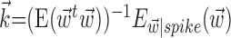, with the first term being the inverse of the correlation matrix of the kinematics vector and the second term being the cross-correlation of with the spike train (the latter reduces to a conditional expectation because of the binary nature of the spike train). When fitting in the absence of kinematic information ( set to 0), we replaced in the above with the neural activity vector ; when fitting and together, is replaced by the vector formed by appending and (other behavioral parameters may be included here by a similar appending operation).

Second, the nonlinear encoding functions were estimated using an intuitive nonparametric binning technique (Chichilnisky, 2001; Shoham, 2001). Briefly, given , for any possible value u of the filtered signal , we found all times {t}_u during the experiment for which was observed to approximately equal u; the conditional firing rate f(u) was then estimated as the fraction of time bins {t}_u that contained a spike (for pictorial representations of this process, see Chichilnisky, 2001; Shoham, 2001). In this procedure, f(u) has an underdetermined scale factor [because a scale factor in the argument u-axis can always be absorbed by rescaling f itself (Chichilnisky, 2001)], which we standardized by mapping the first and 99th quantiles of the observed distributions of u (with u defined as , , or (), depending on the context) to -1 and 1, respectively, in all plots.

To further establish the validity of our results, we compared the filter coefficients calculated using the basic regression-based procedure with ones estimated using alternative, more general methods (Paninski, 2003a), including direct optimization of , with the “modulation function” M(.;.) measuring the total modulation of the firing rate along any arbitrary kinematic filter (for a precise definition of M, see Paninski, 2003a). The alternative methods consistently led to nearly identical solutions (which were, in turn, also insensitive to the precise choice of the modulation function M). The direct optimization method was also used to search for additional modulatory filters (the regression solution provides only one such filter) (see Fig. 5), using , with M now measuring the modulation along the linear subspace spanned by the vectors {} and restricted to be orthogonal to to prevent degeneracy. Again, techniques based on spike-triggered covariance (Brenner et al., 2001; Simoncelli et al., 2004) gave similar results. All plots of estimated firing rates f, and all of the reported information values, are cross-validated (the models were fit using a subset of the data and then tested on a nonover-lapping data subset), ensuring that our analyses provide an accurate summary of how well the model is predicting novel spike trains, not simply reproducing previously observed data. In particular, the effects described here cannot be explained as a result of overfitting to the extra parameters or .

Figure 5.

A single preferred trajectory is sufficient for the representation of the encoding function f. Firing rate of one example cell as a function of two filtered signals, and , with chosen to be the next most informative such filter, restricted to be orthogonal to (see Materials and Methods); y- and x-axes index and , respectively, and color axis indicates the conditional firing rate (in hertz) given these two variables. Contours of firing rate function are approximately linear and perpendicular to the axis: a one-dimensional function captures the relevant structure of the tuning of this neuron (Paninski, 2003a).

Because the hand position and velocity signals varied relatively slowly (the autocorrelation timescale of the velocity was ≥200 msec), we down-sampled these signals to 10 Hz (qualitatively similar results were obtained at higher sampling frequencies). All neural predictions were performed at a much finer timescale (5 msec). Because hand velocity varies much more quickly than the position, we represented the signals and in the velocity domain (with a single position sample added at zero lag for completeness) (see Fig. 2). This permitted us to analyze the preferred trajectory with greater temporal resolution (in mathematical terms, this velocity-based representation is a linear change of basis and therefore entails no loss of information or generality). Tuning quality did not improve with observations of the velocity or position at additional time lags once included lags up to 300 msec before and 500 msec after the current spike bin.

Figure 2.

Diversity of estimated preferred trajectories . Example preferred trajectories , estimated for three different cells. Asterisk indicates contribution of position (in centimeters) at zero time lag, and solid line gives contribution of velocity (in centimeters per second) at the different time lags shown; error bars represent SE. (For why this representation of the preferred trajectory was chosen, see Materials and Methods.)

To further examine and summarize the properties of the encoding nonlinearity, we fit f with various parametric models using maximum likelihood. Several forms for the parametric tuning curves were examined, including power-law, nonsaturating sigmoids, and half-wave rectifying models; the exponential model discussed here was the simplest (smallest number of parameters) that we could find that adequately represented the observed tuning functions, as measured by the likelihood the model assigned to a sufficiently large sample of novel (cross-validated) spike trains. Cells were declared untuned if their (cross-validated) tuning functions were not significantly nonconstant, as measured by a t test comparing the average firing rate observed for positive values of with the rate given negative values. A similar test was constructed for nonlinearity: the test data were split into thirds based on , and we tested whether the firing rate in the rightmost third was significantly greater than a linear extrapolation through the mean firing rates in the leftmost and center thirds. All hypothesis tests were performed at p = 0.05.

We quantified the predictability of the spike train given and/or by computing the expected conditional log-likelihood of observing a spike in a given time bin, normalized by the a priori log-likelihood (that is, the average baseline log-likelihood given no knowledge of or ) (Harris et al., 2003); this expected log-likelihood provides a useful measure of the dependence between these variables and is also known as the mutual information (Cover and Thomas, 1991), as follows:

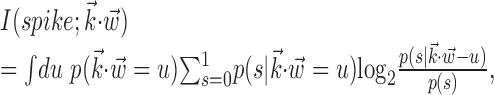with s = 1 or s = 0 depending on whether a spike was observed or not. We chose to use this information-theoretic, likelihood-based measure (rather than, for example, mean-square error or variance-based measures) for three reasons: first, information-theoretic measures are at least as interpretable as the more classical variance-based approaches (Rieke et al., 1997), in many cases agreeing better with common-sense notions of “informativeness” or “noise” (Cover and Thomas, 1991; Rieke et al., 1997) (in particular, the information-theoretic measure does not depend on any linear relationship between the variables of interest); second, likelihood-based methods are intimately connected to modern techniques for analyzing point processes (Brown et al., 2004) (of which spike train data are a canonical example); finally, and most importantly, likelihood-based measures are independent of bin size, whereas variance-based methods depend critically on choosing a proper smoothing factor to estimate the firing rate given a single spike train. In particular, for the small neural bin widths used here, the sparse binary nature of the spike train causes the correlation coefficients between the spike train and the expected firing rate predicted by the model to be misleadingly small. Nevertheless, the reader may compare this with Shoham (2001), who reports correlation coefficients on the order of 0.6 between the predicted activity of the cascade model and suitably time-smoothed versions of the observed spiking activity.

The simple single-filter character of Model 2 makes it easy to compute the information , by simply plugging in the estimated conditional probabilities f into the equation for mutual information (Cover and Thomas, 1991); because the number of data samples (∼10⁵) was much greater than the number of bins (∼10²) in the histogram estimate for f, bias correction of the information estimates was not necessary [bias correction only becomes useful when the number of bins is approximately the same as or larger than the number of samples (Paninski, 2003b)]. It is important to note, however, that the information values given, although represented in units of bits per second for normalization purposes, are not valid estimates of the information rate (Cover and Thomas, 1991) between the dynamic signals spike(t), , and ; the information values presented here (the information between spike(t) and at a single time slice) will in general overestimate the information rate [the information between spike(t) and at all possible time slices, which is generally much more difficult to estimate (Rieke et al., 1997)] because of the strong temporal autocorrelations (redundancies) in these signals. Thus, the values given here should be interpreted as a measure of the statistical dependence between spike, , and and not as a measure of the information-theoretic capacity of the MI network (Paninski et al., 2004).

To determine the minimal number of delay samples needed to represent the information extracted by the full preferred trajectory of a given cell (see Fig. 4), we used the following procedure: first, we chose the optimal single delay τ by maximizing the information [where denotes the two-dimensional hand position sampled at time lag τ] for all τ in the time interval -1 ≤ τ ≤ 1 sec (we found previously this time interval to be sufficient to capture the large majority of optimal delays; cf. Paninski et al., 2004, their Fig. 11). Then we added additional delays iteratively until the cross-validated information stopped growing; similar results were obtained whether or not the delays τ were constrained to be adjacent. The optimal number of delay samples are plotted in histogram form in Figure 4; similar results were obtained by Shoham (2001) using a different technique involving a Bayesian information criterion instead of the cross-validation method used here.

Figure 4.

Information captured as a function of number of delay samples. Top, Each trace corresponds to the information versus number of delay samples for a single cell; asterisk denotes optimal number of delays. Only a randomly chosen subsample of cells is shown here, to avoid overcrowding. Bottom, Histogram of minimal number of filter delays per cell necessary to capture information in full preferred trajectory .

Results

We will describe our findings in terms of the encoding Model 2 introduced in Materials and Methods. Note that this model reduces exactly to the classical expression 1 when the encoding function f has the linear form f(u) = mu + b, the preferred trajectory is restricted to extract only position or velocity at a single time point from the hand-trajectory signal , and the neighboring neural contribution is ignored (i.e., the neural weight vector is set to 0). Thus, the new Model 2 allows us to examine (1) the dependence of MI activity on the full hand trajectory (through the preferred trajectory ) and not just the position or velocity at a fixed time, (2) the nonlinear encoding implemented by MI cells (via f), and (3) the dependence of the firing rate on the activity of neighboring cells in the MI network (via the interneuronal terms ). We discuss each component in turn below.

Preferred trajectory model

The estimated preferred trajectories from three sample cells are shown in Figure 2; the first cell can be approximated as a horizontal position-only encoder, whereas the second encodes a mixture of horizontal position and vertical velocity, and the third the acceleration in the upper right-hand direction (because the velocity weight of this cell is negative at t = 0 and positive at t = 100 msec). The observed preferred trajectories combine kinematic information in a diverse manner; some cells encode strictly position and some strictly velocity, although many encode more complicated combinations of the full trajectory, sampled at multiple time lags.

In Figure 3, we examine the information about firing rate carried by a single sample of (two-dimensional) position or velocity, relative to the information in the full filtered signal . The new model captures significantly more information about the spike train than does either position or velocity alone (Fig. 3, left, middle). In addition, we find velocity-tuned cells to be slightly more prevalent in our population, but most cells provide information about position as well, with some position-tuned cells providing negligible velocity information, supporting and extending previous observations (Ashe and Georgopoulos, 1994) (Fig. 3, right). The lack of any strong clustering in these plots supports the argument that MI cells do not fall into distinct groups of pure velocity or position encoders (Todorov, 2000); a similar lack of clustering is evident if one plots the distribution of weights of position versus velocity or acceleration (that is, the corresponding elements of the preferred trajectory ), because the relationship between these weights is predictive of the informativeness of the cell for these variables (data not shown).

Figure 3.

Scatter plots of information about firing rate from position, versus velocity, versus full filtered signal . Each dot corresponds to the information measured from a single cell (bits per second, measured in 5 msec bins); diagonal line indicates unity. Information estimates in the left and middle panels fall significantly above diagonal, indicating more information provided by optimal than by position or velocity alone. Position was sampled at zero time lag here, with velocity sampled at 100 msec after the current firing rate time bin (lag values chosen to maximize the information values shown; for other time lags, these points tended to fall even farther above the diagonal).

We next investigated the minimal number of delays necessary to capture the information in the full preferred trajectory (Fig. 4). Again, we find a fair degree of heterogeneity (Fig. 4, top): in some cells (∼25% of our population), all of the information in was contained in a single position sample, whereas for others, four or more filter delays were necessary (24 of 122 cells, 20%, met the criterion that the information contained in the optimal number of samples was at least 25% larger than the information contained in the most informative three samples), indicating that these cells are poorly approximated as simple position, velocity, or even position-and-velocity-and-acceleration encoders. Moreover, individual-cell kinematic informativeness is significantly positively correlated with the optimal number of delay samples (Spearman's rank correlation test).

Finally, just as in the linear Model 1, changing the signal in a vector direction orthogonal to the estimated does not significantly modulate the activity of the cell (Fig. 5); the median ratio of information contained in relative to the information in , with being the next most informative filter orthogonal to , was ≥10 (for additional details, see Paninski, 2003a). Thus, a single number, , suffices to capture the modulatory effects of the full dynamic hand trajectory ; in other words, the full encoding surface is well modeled as a (possibly curved) plane, with one main axis (and one corresponding possible vector of curvature), .

Superlinear encoding function

We next characterized the encoding function (Fig. 6). Of the significantly tuned cells (one-sided t test; see Materials and Methods; 109 of 122, or 89%), all but one had monotonic encoding functions f (visual inspection), and approximately one-third of these functions were significantly superlinear (curved upward; one-sided t test; 38 of 109, 35%). Moreover, the degree of superlinearity was strongly correlated with the informativeness of the cell: of the 40 most informative cells in our population, 29 (73%) had significantly superlinear encoding functions. Thus, the cells best modulated by (and most informative about) the hand trajectory signal are the most superlinear.

Figure 6.

Illustration and implications of the nonlinearity of MI cells. a, Example encoding function f (mean ± SE), with corresponding exponential fit. b, Observed encoding function f for filter set to extract optimal , position, or velocity along preferred direction. Tuning becomes sharper (more nonlinear) and observed dynamic range increases as chosen filter becomes closer to optimal . c, Illustration on simulated data of linearization effect on sharpness of nonlinearity. Model cell is perfectly binary, firing with probability one or zero depending on whether is larger or smaller than a threshold value. As the ratio of to becomes larger (i.e., as we project onto an axis that is farther away from the true ), the observed nonlinearity becomes shallower and smoother, becoming perfectly flat in the limit as becomes large. d, Dependence of velocity direction tuning curves (expected firing rate as a function of velocity angle) on hand position. Gray curve was computed using only velocities that were observed when hand position was to the left of midline; black curve used only rightward positions. Cosine curve (dashed) shown for comparison; observed tuning is significantly sharper than cosine (one-sided t test).

We found that this nonlinearity was well fit by a simple exponential model f(u) = be^mu (with u abbreviating , the slope parameter m being an index of tuning strength, and b again denoting the baseline firing rate): this exponential model predicted novel spike trains as well as or better than the full histogram model (Fig. 6a,b, dark traces) in 83% (90 of 109) of our significantly tuned cells, with only a median 5% log-likelihood loss in the remaining 19 cells. As expected, the tuning strength parameter m was significantly correlated with both the informativeness of the cell and its degree of superlinearity. Thus, the relevant tuning structure in f was captured sufficiently well by a highly compact two-parameter function.

This superlinearity has some important implications for the tuning properties of MI cells, as illustrated in Figure 6. First, the degree to which a cell will appear to code the movement signal superlinearly will depend strongly on the agreement between the chosen prefilter and the true preferred trajectory of the cell. To see why, imagine a neuron whose firing rate is exactly described by Model 2: for this hypothetical cell, tuning will be strongest and most superlinear along the vector , because the tuning along any other vector (, for example, with orthogonal to ) will be made smoother and shallower (that is, more linear and with a smaller slope, or gain) by the addition of the component which (like in Fig. 5) does not modulate the firing rate of the cell and hence effectively acts as a noise term. Figure 6c provides a simple demonstration of this effect using simulated data (for additional mathematical details, see Paninski, 2003a). In the extreme case when the noise term dominates the tuned component , the cell appears to be completely untuned, with a constant encoding function f (that is, linear, with 0 slope).

An example of this linearization effect in our neural data is given in Figure 6b. The neuron shown here appears to encode position fairly linearly; only when we choose to be the preferred trajectory does the full superlinear behavior of the cell become apparent. Of our significantly superlinear cells, only 33% had significantly superlinear encoding functions f when was allowed to extract just the preferred (two-dimensional) velocity at a single time point (median ratio of full kinematic model m to position-only and velocity-only model m: 2.8 and 1.9, respectively; both significantly ≥1, one-sided t test).

Second, the near-planar form of the observed encoding surfaces (Fig. 5) is, in a sense, the origin for the familiar near-sinusoidal shape of velocity directional tuning curves (mean firing rate as a function of the hand velocity angle), for the same reason that the exactly planar encoding surfaces in Model 1 lead to exactly cosine velocity directional tuning curves. In addition, Model 2 predicts that, for cells with superlinear f, these tuning curves will generally peak more sharply than the cosine function (Fig. 6d), because superlinear encoding functions f will “stretch out” the tuning curve vertically, thus sharpening its peak. We found that the median width at half-height of these curves was 0.83π radians, significantly less than π, the width expected of sinusoidal tuning (one-sided t test); moreover, the tuning strength parameter m was significantly negatively correlated with the tuning curve width (Spearman's rank correlation test).

Third, the superlinear, approximately exponential form of the observed encoding functions f predicts that velocity direction tuning curves will depend approximately multiplicatively on the position of the hand (and vice versa), even during continuously varying behavior (Caminiti et al., 1990; Scott and Kalaska, 1997; Sergio and Kalaska, 2003). (This prediction follows from the fact that the exponential function converts addition into multiplication, i.e., the linear filter term , which adds the position and velocity contributions, is converted into , which multiplies the position and velocity contributions.) To test for this effect (Fig. 6d), we constructed two tuning curves for velocity direction: one computed using only the half of the velocity data recorded while the hand position was positively oriented with (that is, ), and the other when the hand was in the opposite (negative) half of the workspace. Although the median position difference between these two conditions was quite small (3.5 cm), the positive-position tuning curve was modulated by a factor of 3 over the negative in the cell shown in Figure 6d. Of our 38 significantly superlinear cells, 11 (29%) showed a modulation factor of >50%; the median modulation in superlinear cells was 16%. Finally, this modulation factor was significantly correlated with the tuning strength m in our tuned cell population.

Figure 7 illustrates this gain-modulation effect from a different point of view. Here we compare the firing rate predicted by the full superlinear kinematic encoding model with the rate predicted by three simpler models: the optimal linear model (fit by standard linear regression), the optimal nonlinear model based only on a single (two-dimensional) position sample, and the optimal nonlinear single-sample velocity model (for additional comparisons, see Shoham, 2001). Three features of these predictions are clearly visible: first, the optimal full superlinear model resembles the optimal linear model in the moderate-activity regimen (≈1-10 Hz). However, the superlinear prediction, as expected, displays a strong expansion for higher firing rates (as visible in Fig. 6) and compression for low firing rates (in which the linear firing rate prediction often becomes negative); this increased dynamic range leads to improved predictions [note the increased similarity between the predicted firing rate of the full model and the distribution of spikes in the observed spike train in Fig. 7, bottom; more quantitatively, for this cell, the full information was greater than twice that available in either position or velocity alone, a not atypical case given Fig. 3]. Finally, the full superlinear prediction for this cell is approximately proportional to the product of the position- and velocity-only predictions: the full-kinematic trace follows the rapid variations of the velocity trace, modulated by the slower changes of the position, which acts generally like a gain signal here.

Figure 7.

Comparison of firing rate predictions; example of multiplicative gain-modulation effect. Top, Firing rates predicted by full nonlinear kinematic model, best linear model, best nonlinear velocity model, and best nonlinear position model. Bottom, True observed spike train (asterisks) and time-smoothed firing rate (solid). Firing rate smoothed here with a Gaussian kernel for which the width was chosen to approximately match the timescale of firing rate variations in top panel (for straightforward comparisons).

We summarize the kinematic encoding properties of the model in Figure 8. The top row shows a “spatiotemporal” tuning function (STTF) for velocity; this is the mean observed firing rate of a single cell, given the (two-dimensional) velocity at a time sample τ seconds in the future (Paninski et al., 2004). In the middle row is the STTF predicted by Model 2; despite its simplicity and small number of free parameters, Model 2 accounts for all of the major features of the observed STTF, including the onset and offset of the strongest tuning (at τ ≈ 100 msec), the relative strength, approximately planar shape, and orientation of the spatial tuning function at each time lag; finally, surrogate STTFs, constructed using simulated spike trains sampled from the model, mimic the observed variability in the STTF (Fig. 8, bottom).

Figure 8.

Comparison of observed and model spatiotemporal tuning functions. Top, Observed STTF; mean firing rate of a single cell, given the (two-dimensional) velocity τ seconds in the future (Paninski et al., 2004). Middle, Modeled STTF constructed from average firing rate predicted by Model 2. Bottom, Simulated STTF constructed by stochastically sampling spike trains from Model 2.

Instead of a single PD per neuron, Model 2 effectively incorporates a sequence of PDs, varying with the time lag τ (Baker et al., 1997). As found by Paninski et al. (2004), MI STTFs typically show a particularly simple form of PD dependence on τ: in the context of tracking behavior, PDs essentially do not rotate as a function of τ but rather are modulated in gain, with possible flips when the gain modulation becomes negative. Hints of more complex rotational behavior are occasionally exposed by the analysis of Figure 8 (see especially the middle row; however, note that this more subtle rotational behavior was always weak and was only visible in a minority of our cells, consistent with the results of Paninski et al., 2004). Across our cell population, the model-based STTF predicts the observed STTF >50% more accurately (in the sense of squared error), on average, than does the real STTF constructed from held-out training data (essentially because the model provides a smoother, less-variable STTF than is available from the original binned neural data). In summary, Model 2 provides a description of MI kinematic tuning that is both more accurate and more compact than was available previously.

Interneuronal dependencies

The final component of Model 2 involves the ongoing network activity in neighboring cells, (Fig. 9). To begin, we consider this neighbor activity in the absence of kinematic information, i.e., set to 0 in Model 2. In our full cell population, the network activity gives approximately the same amount of information as does an instantaneous sample of the hand position or velocity (Fig. 9a), despite the fact that we are observing fewer than 25 cells, a tiny fraction of the full MI neural network. (This figure compares with velocity information, but the corresponding plot for position is qualitatively similar; recall Figure 2.) Because noisy transformations always decrease information (Cover and Thomas, 1991), this finding contradicts the view of MI activity as a simple noisy transformation of the hand velocity; a straightforward explanation is that MI cells are correlated because of common sources of excitation beyond that expected from overlaps in velocity tuning alone (i.e., overlaps in the full preferred trajectory ) and not because of interneuronal interactions per se (Hatsopoulos et al., 1998; Lee and Georgopoulos, 1998; Oram et al., 2001). This argument is supported by a comparison of the scales of Figures 9a and 3: the neural ensemble information tends to be smaller than the full kinematic information . Moreover, the interneuronal weights (when fit in the absence of kinematic information, ) are highly correlated with the overlap in the preferred trajectory [data not shown; “overlap” measured here by , the vector angle between the preferred trajectory of the target cell and that of cell i]. As expected, this kinematic overlap was a strong predictor of the information one cell would carry about another (Spearman's rank correlation test), and the informativeness of the network alone, was positively correlated with the number of cells observed (Nicolelis et al., 2003; Paninski et al., 2004).

Figure 9.

Observing neighbor activity increases the predictability of MI neurons. a, Comparison of information values for neural-only (no kinematic input; ) versus velocity-only (no neural input; ) models. Conventions as in Figure 2; for fair comparison, information values here are based on the largest bin width shown in d, 500 msec. b, Comparison of information values for full model (kinematic data augmented with neighboring neural activity ) versus kinematic-only model (). Significantly more points fall above the equality line (one-sided t test; note logarithmic scale used to expose structure in scatter plot here). c, Estimated encoding functions f for kinematic-only (gray trace) versus full model (black). Note the differences in dynamic range of two curves. Cell illustrated here is marked with an “x” in b. d, Effects of bin width on network informativeness in the presence of kinematic information [ nonzero; solid trace is median ± SE information difference over all cells, plotted against bin width used to define n_i] and without [dashed trace is , i.e., ].

What happens when both neural and kinematic information are included in the model (i.e., and nonzero) simultaneously? We found that observing can significantly increase the predictability of the activity of a given cell, even if one has already observed the full kinematic signal [the information difference is significantly positive; one-sided t test] (Fig. 9b); nonetheless, this increase is of relatively small magnitude overall. Close examination of Figure 9b reveals two generally distinct subpopulations: most cells show no significant information increase given the observation of (indeed, many display a slight decrease of information as a result of overfitting effects); however, 16 of our 109 tuned cells (15%) do show a significant increase (in which significance is empirically defined as the negative of the envelope containing all of the negative information-difference points, extending down to approximately -0.025 bits/sec). An example is shown in Figure 9c; for this cell, inclusion of significantly increased the predictability of the spike train, as measured by mutual information and by the dynamic range of the observed encoding function f. To give a sense of scale, the cell illustrated here has an information difference (cf. Fig. 9b) of 0.07 bits/sec. The information gained by appending to is invariably approximately one order of magnitude smaller than that available from the kinematic signal alone; thus, the distribution of changes in information is mainly skewed to positive values rather than strongly shifted toward the positive.

Finally, when we examine the relationship between the informativeness of a cell and the bin size over which we observe n_i (Fig. 9d), the information value of the neural-only model slowly increases as n_i is allowed to average over a larger time bin, up to an asymptote at 500 msec (i.e., where n_i(t) is defined as the spike count in the interval [-250, 250 msec] before and after the current 5 msec time bin t). In addition, a significantly large (t test) proportion of cells show an information increase when the bin size is increased between any of the bin widths shown in Figure 9d: 10, 50, 100, 200, and 500 msec. This increase of information with bin size is expected, because counting spikes over a larger time period should increase the information; the observed slow growth of this neural ensemble information with bin size may be interpreted as reflecting the long autocorrelation timescale of the MI network driven by the underlying kinematics .

A different pattern is evident when considering the full kinematic-and-ensemble information : the information difference shown in Figure 9d increases quickly with bin size, reaching a maximum by 100 msec, with a statistically insignificant slight decrease as the bin width increases beyond 200 msec. Thus, in contrast to the neural-only case (), observing the neighbor spike trains over time windows of length greater than ≈100 msec does not enhance the predictability of the activity of the cell. In addition, the interneuronal weights a_i were correlated much more weakly (although still significantly; Spearman's rank correlation test) with the kinematic vector angle overlap when fit in the presence of kinematic information ( nonzero) than in its absence ().

Discussion

We have presented a compact description of the nonlinear population encoding of hand trajectory in MI. This description, a direct generalization of the canonical cosine-tuning Model 1, provides more accurate predictions of MI activity and captures several novel aspects of MI coding: the heterogeneity of the preferred trajectories ; the superlinearity of the encoding function f (and the gain-modulation implications thereof); and the precise relevance of interneuronal dependencies beyond simple pairwise correlations. Each of these components has been discussed previously in some form in the literature; our contribution is a detailed quantification of these effects and a synthesis into a well-defined, compact statistical model.

Preferred trajectory model

Our results are based on a statistical cascade model of spiking activity, with a linear filtering stage (typically interpreted as a “receptive field” in sensory studies and interpretable as a preferred trajectory here) followed by a probabilistic nonlinearity (Yamada and Lewis, 1999; Brenner et al., 2001; Chichilnisky, 2001; Shoham, 2001; Touryan et al., 2002; Paninski, 2003a; Simoncelli et al., 2004). This cascade analysis allowed us to simultaneously model the combination of multiple kinematic parameters from all relevant time delays, in an optimal and parsimonious way; this “global” approach is necessary for the accurate modeling of MI activity, which multiplexes diverse kinematic parameters with heterogeneous time delays (Georgopoulos et al., 1984, 1986; Porter and Lemon, 1993; Moran and Schwartz, 1999; Sergio and Kalaska, 2003; Paninski et al., 2004), allowing MI to both predict motor output and encode sensory feedback.

Our findings on the heterogeneity of MI tuning and the relative contributions of velocity and position to MI activity (Figs. 2, 3) are consistent with previous results using multiple-regression techniques (Ashe and Georgopoulos, 1994; Fu et al., 1995). Our previous work (Paninski et al., 2004) quantified similar observations on the “spatiotemporal” tuning properties of MI cells, using information-theoretic tools instead of the correlation-based methods used previously; we extended this work here by examining how best to combine the hand position or velocity at multiple time lags (Fig. 4) and not just individual lags as used by Paninski et al. (2004). Figure 8 illustrates that the current approach provides an equivalent but simpler account of MI spatiotemporal tuning properties. Although the filter-based Model 2 might appear more complex than the classical Model 1, Model 2 is really no more difficult to use because of the simplicity of the linear filtering operation; as noted above, the linear Model 1 is a special case of Model 2.

Our results are also related to spike-triggered averaging work (Fetz and Cheney, 1980; Morrow and Miller, 2003) connecting MI spikes to peripheral muscle activity. It will be important to dissociate these effects and quantify their relative importance for MI activity, as performed here for kinematic parameters and network activity; very similar modeling methods could be applied to the analysis of EMG and other behaviorally relevant signals, including, for example, forces, joint angles, and torques (Evarts, 1968; Humphrey et al., 1970; Kakei et al., 1999).

Superlinear encoding function

The cascade methodology allows us to coherently combine different kinematic features to predict neural activity. Even more importantly, these techniques generalize previous attempts to model these cells using multiple-regression methods (Ashe and Georgopoulos, 1994; Fu et al., 1995), by allowing us to discover and quantify, in a nonparametric (relatively assumption-free) way, the nonlinear effects of these variables on MI activity. We found that approximately one-third of MI cells (and the majority of the best-tuned cells) encode the trajectory signal superlinearly. This superlinearity, in turn, has important implications for more classical descriptions of the MI neural code (Fig. 6); the superlinearity was reasonably well modeled by a simple exponential transformation that sharpens MI directional tuning and leads to a “gain modulation” effect whereby the dependence of neural activity on velocity is modulated, approximately multiplicatively, by the hand position. This result bears an interesting resemblance to recent work by Hwang et al. (2003), who modeled their psychophysical results using multiplicative interactions between hand position and velocity; thus, our results could indicate a neuronal correlate of multiplicative gain-modulated encoding at the behavioral level.

Similar nonlinearities in MI tuning have been observed in the literature but, to our knowledge, never investigated systematically. Rectification effects have been noted while fitting linear surfaces to MI activity (Kettner et al., 1988; Todorov, 2000) (compare with the negativity of the linear prediction in Fig. 7). Our finding that superlinearity leads to sharper-than-cosine directional tuning curves (Fig. 6c) is consistent with the results of Amirikian and Georgopoulos (2000), who observed similarly “stretched” tuning curves during reaching behavior; indeed, their exponential-cosine model (Amirikian and Georgopoulos, 2000, their expression 4) is the analog, in velocity direction-tuning space, of our multivariate Model 2. Similarly, Schwartz and colleagues (Moran and Schwartz, 1999) found tuning asymmetries between the preferred and opposite velocity directions (indicating similarly stretched deviations from sinusoidal tuning).

Note that the strength of this superlinearity is probably underestimated here. The superlinearity is partially obscured when one considers only the instantaneous hand position or velocity and not the full hand trajectory (Fig. 6); this “masking” effect of choosing the non-optimal prefilter helps explain why these superlinearities have been underemphasized previously. Conversely, including information about joint angles, torques, or other behaviorally relevant parameters could expose stronger, possibly qualitatively different, nonlinearity. Different behavioral settings might also expose additional nonlinearity, e.g., if the observed range of is increased [because functions that appear quasi-linear over a small range of might be strongly nonlinear over larger scales].

Somewhat surprisingly, we found little nonlinear structure in the encoding surfaces in vector directions orthogonal to ; these surfaces have a simple, near-planar form, with just one possible vector of (upward) curvature (Fig. 5). In the sensory domain, in contrast, encoding surfaces with multiple axes of curvature (along several receptive field-like vectors) are frequently observed (Yamada and Lewis, 1999; Brenner et al., 2001; Touryan et al., 2002; Rust et al., 2003). For example, complex cells in the visual cortex are poorly modeled using the simple form Model 2, because of the approximate phase-invariance of their responses; instead, they are typically modeled using an expression such as , with the receptive fields , separated in-phase by 90° and f, a bowl-shaped (highly nonplanar) function [e.g., f(u, v) = u² + v² (Simoncelli and Heeger, 1998)]. Again, additional nonlinearity might plausibly be exposed after observing additional kinematic parameters; for example, Caminiti et al. (1990), Scott and Kalaska (1997), and Sergio and Kalaska (2003) observed not just gain-modulation effects but rotation of preferred velocity directions under perturbations of the arm posture larger than those considered here.

The physiological origin of this superlinearity is currently uncertain. Biomechanical models of the motor plant predict nonlinear relationships between cortical activity and kinematic parameters (Mussa-Ivaldi, 1988; Todorov, 2000); other biophysical sources of nonlinearity could include voltage-dependent sub-threshold currents and network dynamics. Meanwhile, computational implications for gain-modulated coding have been studied extensively (Zipser and Andersen, 1988; Pouget and Sejnowski, 1997; Salinas and Abbott, 2001); this previous work has argued that multiplicative gain fields represent a neurophysiologically plausible mechanism for implementing coordinate transformations between representations of sensory inputs and motor outputs. Our evidence for the presence of gain fields could therefore indicate motor cortical involvement in sensorimotor transformations, with MI operating as a computational (not solely representational) map. Finally, the simple, monotonic form of the observed nonlinearity seems advantageous for controlling the multiple interdependent parameters underlying coordinated movement (Mussa-Ivaldi, 1999).

Interneuronal dependencies

Recent technological advances have enabled simultaneous recordings from many individual neurons (Cossart et al., 2003; Harris et al., 2003; Nicolelis et al., 2003), necessitating the development of methods capable of deciphering this complex population data. We have introduced techniques here for studying the individual tuning functions beyond incorporaon of just pairwise correlations; knowledge of these individual functions, in turn, allows us (via Bayes' rule) to investigate the full population code , the probability of observing any given activity pattern as a function of the input . Our results complement previous findings on pairwise dependencies in MI (Riehle et al., 1997; Hatsopoulos et al., 1998; Lee and Georgopoulos, 1998; Maynard et al., 1999; Baker et al., 2001) and more general dependencies in visual cortex (Arieli et al., 1996; Tsodyks et al., 1999) and hippocampus (Harris et al., 2003): the activity of a cortical cell depends on that of its neighbors, and a complete understanding of the cortical code requires explicit modeling of these interdependencies (Chornoboy et al., 1988; Yang and Shamma, 1990; Martignon et al., 2000; Brown et al., 2004).

We examined these dependencies in two distinct contexts: in the absence and presence of information about the current kinematic state of the arm. The neural-only analysis () indicated significant redundancy in MI, with neurons carrying large amounts of information about the correlated population activity of their neighbors; these results are consistent with the view that MI cells share common sources of excitation that encode complex functions of the movement trajectory kinematics. The analysis in the context of observed kinematic information ( nonzero) went further, demonstrating that these interneuronal dependencies remain significant even when accounting for the “common input” . Moreover, the preferred timescale of the interneuronal spike counts n_i is much shorter in the presence of kinematic information than in its absence (Fig. 9d). Finally, the correlation between the interneuronal weights a_i and the overlap in is greatly reduced by the inclusion of kinematic information, all indicating that these dependencies are not just attributable to overlaps in kinematic preference. Thus, the activity of a given neuron must be interpreted in the context of the activity of neighboring cells in the MI network.

Nevertheless, although significant, the differential effect of these dependencies is small compared with the information in the trajectory signal (Fig. 9b; similar results are obtained using different techniques by Truccolo et al., 2003). Thus, whereas the interneuronal term plays a significant role in our Model 2, the kinematic term tends to dominate. In both aspects, our findings complement the literature on correlations between pairs of MI neurons (Smith and Fetz, 1989; Riehle et al., 1997; Hatsopoulos et al., 1998; Lee and Georgopoulos, 1998; Maynard et al., 1999; Baker et al., 2001; Oram et al., 2001): although correlations within the MI neural network are strong, much (although not all) of this interneuronal dependency can be accounted for by overlaps in kinematic preferences. Future work will examine the implications for the “decoding” problem inherent in the design of neural-prosthetic devices (Donoghue, 2002; Mussa-Ivaldi and Miller, 2003; Nicolelis et al., 2003; Brockwell et al., 2004).

We may contrast our results to those of Harris et al. (2003), who examined interneuronal dependencies in the hippocampus using related techniques. Their analysis found these hippocampal dependencies to be much less locked to external kinematic parameters than those we observe in MI; moreover, the optimal timescale for hippocampal dependencies was much smaller (≈20 msec) (cf. Fig. 9d), with a better-resolved peak at the optimal bin width. Together, these results indicate striking differences in the population codes of MI and hippocampus, which in turn could reflect differences in their underlying computational architectures (e.g., the relative roles of redundancy reduction and signal averaging) (for additional discussion, see Harris et al., 2003).

References

- Adrian E (1926) The impulses produced by sensory nerve endings. J Physiol (Lond) 61: 49-72. [DOI] [PMC free article] [PubMed] [Google Scholar]
- Amirikian B, Georgopoulos A (2000) Directional tuning profiles of motor cortical cells. Neuroscience Res 36: 73-79. [DOI] [PubMed] [Google Scholar]
- Arieli A, Sterkin A, Grinvald A, Aertsen A (1996) Explanation of the large variability in evoked cortical responses. Science 273: 1868-1871. [DOI] [PubMed] [Google Scholar]
- Ashe J, Georgopoulos A (1994) Movement parameters and neural activity in motor cortex and area 5. Cereb Cortex 4: 590-600. [DOI] [PubMed] [Google Scholar]
- Baker J, Fellows M, Donoghue J (1997) Directional tuning rotations in motor cortical neurons during radial arm movements. Soc Neurosci Abstr 23: 607.2. [Google Scholar]
- Baker S, Spinks R, Jackson A, Lemon R (2001) Synchronization in monkey motor cortex during a precision grip task. J Neurophysiol 85: 869-885. [DOI] [PubMed] [Google Scholar]
- Brenner N, Bialek W, de Ruyter van Steveninck R (2001) Adaptive rescaling optimizes information transmission. Neuron 26: 695-702. [DOI] [PubMed] [Google Scholar]
- Brockwell A, Rojas A, Kass R (2004) Recursive Bayesian decoding of motor cortical signals by particle filtering. J Neurophysiol 91: 1899-1907. [DOI] [PubMed] [Google Scholar]
- Brown E, Kass R, Mitra P (2004) Multiple neural spike train data analysis: state-of-the-art and future challenges. Nat Neurosci 7: 456-461. [DOI] [PubMed] [Google Scholar]
- Caminiti R, Johnson P, Urbano A (1990) Making arm movements within different parts of space: dynamic aspects in the primate motor cortex. J Neurosci 10: 2039-2058. [DOI] [PMC free article] [PubMed] [Google Scholar]
- Chichilnisky E (2001) A simple white noise analysis of neuronal light responses. Network 12: 199-213. [PubMed] [Google Scholar]
- Chornoboy E, Schramm L, Karr A (1988) Maximum likelihood identification of neural point process systems. Biol Cybern 59: 265-275. [DOI] [PubMed] [Google Scholar]
- Cossart R, Aronov D, Yuste R (2003) Attractor dynamics of network up states in the neocortex. Nature 423: 283-288. [DOI] [PubMed] [Google Scholar]
- Cover T, Thomas J (1991) Elements of information theory. New York: Wiley.
- Donoghue J (2002) Connecting cortex to machines: recent advances in brain interfaces. Nat Neurosci 5: 1085-1088. [DOI] [PubMed] [Google Scholar]
- Evarts E (1968) Relation of pyramidal tract activity to force exerted during voluntary movement. J Neurophysiol 31: 14-27. [DOI] [PubMed] [Google Scholar]
- Fetz E, Cheney P (1980) Postspike facilitation of forelimb muscle activity by primate corticomotoneuronal cells. J Neurophysiol 44: 751-772. [DOI] [PubMed] [Google Scholar]
- Fu Q, Flament D, Coltz J, Ebner T (1995) Temporal encoding of movement kinematics in the discharge of primate primary motor and premotor neurons. J Neurophysiol 73: 836-854. [DOI] [PubMed] [Google Scholar]
- Georgopoulos A, Kalaska J, Caminiti R, Massey J (1982) On the relations between the direction of two-dimensional arm movements and cell discharge in primate motor cortex. J Neurosci 2: 1527-1537. [DOI] [PMC free article] [PubMed] [Google Scholar]
- Georgopoulos A, Caminiti R, Kalaska J (1984) Static spatial effects in motor cortex and area 5: quantitative relations in a two-dimensional space. Exp Brain Res 54: 446-454. [DOI] [PubMed] [Google Scholar]
- Georgopoulos A, Kettner R, Schwartz A (1986) Neuronal population coding of movement direction. Science 233: 1416-1419. [DOI] [PubMed] [Google Scholar]
- Harris K, Csicsvari J, Hirase H, Dragoi G, Buzsaki G (2003) Organization of cell assemblies in the hippocampus. Nature 424: 552-556. [DOI] [PubMed] [Google Scholar]
- Hatsopoulos N, Ojakangas C, Paninski L, Donoghue J (1998) Information about movement direction obtained by synchronous activity of motor cortical neurons. Proc Natl Acad Sci USA 95: 15706-15711. [DOI] [PMC free article] [PubMed] [Google Scholar]
- Humphrey D, Schmidt E, Thompson W (1970) Predicting measures of motor performance from multiple cortical spike trains. Science 170: 758-762. [DOI] [PubMed] [Google Scholar]
- Hwang E, Donchin O, Smith M, Shadmehr R (2003) A gain-field encoding of limb position and velocity in the internal model of arm dynamics. PLoS Biol 1: E25. [DOI] [PMC free article] [PubMed] [Google Scholar]
- Kakei S, Hoffman D, Strick P (1999) Muscle and movement representations in the primary motor cortex. Science 285: 2136-2139. [DOI] [PubMed] [Google Scholar]
- Kettner R, Schwartz A, Georgopoulos A (1988) Primate motor cortex and free arm movements to visual targets in three-dimensional space. III. Positional gradients and population coding of movement direction from various movement origins. J Neurosci 8: 2938-2947. [DOI] [PMC free article] [PubMed] [Google Scholar]
- Lee D, Georgopoulos A (1998) Variability and correlated noise in the discharge of neurons in motor and parietal areas of the primate cortex. J Neurosci 18: 1161-1170. [DOI] [PMC free article] [PubMed] [Google Scholar]
- Martignon L, Deco G, Laskey K, Diamond M, Freiwald W, Vaadia E (2000) Neural coding: higher-order temporal patterns in the neurostatistics of cell assemblies. Neural Comput 12: 2621-2653. [DOI] [PubMed] [Google Scholar]
- Maynard E, Hatsopoulos N, Ojakangas C, Acuna B, Sanes J, Normann R, Donoghue J (1999) Neuronal interactions improve cortical population coding of movement direction. J Neurosci 19: 8083-8093. [DOI] [PMC free article] [PubMed] [Google Scholar]
- Moran D, Schwartz A (1999) Motor cortical representation of speed and direction during reaching. J Neurophysiol 82: 2676-2692. [DOI] [PubMed] [Google Scholar]
- Morrow M, Miller L (2003) Prediction of muscle activity by populations of sequentially recorded primary motor cortex neurons. J Neurophysiol 89: 2279-2288. [DOI] [PMC free article] [PubMed] [Google Scholar]
- Mussa-Ivaldi F (1988) Do neurons in the motor cortex encode movement direction? An alternative hypothesis. Neurosci Lett 91: 106-111. [DOI] [PubMed] [Google Scholar]
- Mussa-Ivaldi F (1999) Modular features of motor control and learning. Curr Opin Neurobiol 9: 713-717. [DOI] [PubMed] [Google Scholar]
- Mussa-Ivaldi F, Miller L (2003) Brain-machine interfaces: computational demands and clinical needs meet basic neuroscience. Trends Neurosci 26: 329-334. [DOI] [PubMed] [Google Scholar]
- Nicolelis M, Dimitrov D, Carmena J, Crist R, Lehew G, Kralik J, Wise S (2003) Chronic, multisite, multielectrode recordings in macaque monkeys. Proc Natl Acad Sci USA 100: 11041-11046. [DOI] [PMC free article] [PubMed] [Google Scholar]
- Oram M, Hatsopoulos N, Richmond B, Donoghue J (2001) Excess synchrony in motor cortical neurons provides redundant direction information with that from coarse temporal measures. J Neurophysiol 86: 1700-1716. [DOI] [PubMed] [Google Scholar]
- Paninski L (2003a) Convergence properties of some spike-triggered analysis techniques. Network 14: 437-464. [PubMed] [Google Scholar]
- Paninski L (2003b) Estimation of entropy and mutual information. Neural Comput 15: 1191-1253. [Google Scholar]
- Paninski L, Fellows M, Hatsopoulos N, Donoghue J (2004) Spatiotemporal tuning properties for hand position and velocity in motor cortical neurons. J Neurophysiol 91: 515-532. [DOI] [PubMed] [Google Scholar]
- Porter R, Lemon R (1993) Corticospinal function and voluntary movement. Oxford: Clarendon.
- Pouget A, Sejnowski T (1997) Spatial transformations in the parietal cortex using basis functions. J Cognit Neurosci 9: 222-237. [DOI] [PubMed] [Google Scholar]
- Riehle A, Grun S, Diesmann M, Aertsen A (1997) Spike synchronization and rate modulation differentially involved in motor cortical function. Science 278: 1950-1953. [DOI] [PubMed] [Google Scholar]
- Rieke F, Warland D, de Ruyter van Steveninck R, Bialek W (1997) Spikes: exploring the neural code. Cambridge, MA: MIT.
- Rust N, Schwartz O, Movshon A, Simoncelli E (2003) Spike-triggered characterization of excitatory and suppressive stimulus dimensions in monkey v1 directionally selective neurons. Paper presented at the 12th Annual Computational Neuroscience Meeting, Alicante, Spain, July.
- Salinas E, Abbott L (2001) Coordinate transformations in the visual system: how to generate gain fields and what to compute with them. In: Principles of neural ensemble and distributed coding in the nervous system (Nicolelis MAL, ed), pp 175-190. Amsterdam: Elsevier. [DOI] [PubMed]
- Scott S, Kalaska J (1997) Reaching movements with similar hand paths but different arm orientations. I. Activity of individual cells in motor cortex. J Neurophysiol 77: 826-852. [DOI] [PubMed] [Google Scholar]
- Sergio L, Kalaska J (2003) Systematic changes in motor cortex activity with arm posture during directional isometric force generation. J Neurophysiol 89: 212-228. [DOI] [PubMed] [Google Scholar]
- Serruya M, Hatsopoulos N, Paninski L, Fellows M, Donoghue J (2002) Instant neural control of a movement signal. Nature 416: 141-142. [DOI] [PubMed] [Google Scholar]
- Shoham S (2001) Advances towards an implantable motor cortical interface. PhD thesis, University of Utah; available at http://www.princeton.edu/~sshoham/Shoham_dissertation01.pdf.
- Simoncelli EP, Heeger DJ (1998) A model of neuronal responses in visual area MT. Vision Res 38: 743-761. [DOI] [PubMed] [Google Scholar]
- Simoncelli E, Paninski L, Pillow J, Schwartz O (2004) Characterization of neural responses with stochastic stimuli. In: The cognitive neurosciences, Ed 3 (Gazzaniga M, ed). Cambridge, MA: MIT, in press.
- Smith W, Fetz E (1989) Effects of synchrony between primate corticomotoneuronal cells on post-spike facilitation of muscles and motor units. Neurosci Lett 96: 76-81. [DOI] [PubMed] [Google Scholar]
- Todorov E (2000) Direct cortical control of muscle activation in voluntary arm movements: a model. Nat Neurosci 3: 391-398. [DOI] [PubMed] [Google Scholar]
- Touryan J, Lau B, Dan Y (2002) Isolation of relevant visual features from random stimuli for cortical complex cells. J Neurosci 22: 10811-10818. [DOI] [PMC free article] [PubMed] [Google Scholar]
- Truccolo W, Eden U, Fellows M, Donoghue J, Brown E (2003) Multivariate conditional intensity models for motor cortex. Neural encoding and decoding of discrete and continuous movements. Soc Neurosci Abstr 29: 607.11. [Google Scholar]
- Tsodyks M, Kenet T, Grinvald A, Arieli A (1999) Linking spontaneous activity of single cortical neurons and the underlying functional architecture. Science 286: 1943-1946. [DOI] [PubMed] [Google Scholar]
- Yamada W, Lewis E (1999) Predicting the temporal responses of non-phase-locking bullfrog auditory units to complex acoustic waveforms. Hearing Res 130: 155-170. [DOI] [PubMed] [Google Scholar]
- Yang X, Shamma S (1990) Identification of connectivity in neural networks. Biophys J 57: 987-999. [DOI] [PMC free article] [PubMed] [Google Scholar]
- Zipser D, Andersen R (1988) A back-propagation programmed network that simulates response properties of a subset of posterior parietal neurons. Nature 331: 679-684. [DOI] [PubMed] [Google Scholar]