Identification of Multiple Kinetic Populations of DNA-Binding Proteins in Live Cells

Abstract

Understanding how multiprotein complexes function in cells requires detailed quantitative understanding of their association and dissociation kinetics. Analysis of the heterogeneity of binding lifetimes enables the interrogation of the various intermediate states formed during the reaction. Single-molecule fluorescence imaging permits the measurement of reaction kinetics inside living organisms with minimal perturbation. However, poor photophysical properties of fluorescent probes limit the dynamic range and accuracy of measurements of off rates in live cells. Time-lapse single-molecule fluorescence imaging can partially overcome the limits of photobleaching; however, limitations of this technique remain uncharacterized. Here, we present a structured analysis of which timescales are most accessible using the time-lapse imaging approach and explore uncertainties in determining kinetic subpopulations. We demonstrate the effect of shot noise on the precision of the measurements as well as the resolution and dynamic range limits that are inherent to the method. Our work provides a convenient implementation to determine theoretical errors from measurements and to support interpretation of experimental data.

Significance

Measuring lifetimes of interactions between DNA-binding proteins and their substrates is important for understanding how they function in cells. In principle, time-lapse imaging of fluorescently tagged proteins using single-molecule methods can be used to identify multiple subpopulations of DNA-binding proteins and determine binding lifetimes lasting for several tens of minutes. Despite this potential, currently available guidelines for the selection of binding models are unreliable, and the practical implementation of this approach is limited. Here, using experimental and simulated data, we identify the minimal size of the data set required to resolve multiple populations reliably and measure binding lifetimes with desired accuracy. This work serves to provide a guide to data collection and measurement of DNA-binding lifetimes from single-molecule time-lapse imaging data.

Introduction

Understanding fundamental processes of life requires the characterization of the kinetics of interactions between biological molecules. At single-molecule levels, these systems often exhibit kinetic heterogeneity that is inherent to the presence of multiple intermediate states (1, 2, 3, 4, 5, 6, 7, 8, 9, 10, 11, 12, 13, 14, 15, 16, 17). Advances in single-molecule imaging have enabled the detection and characterization of heterogeneous subpopulations in reactions conducted in vitro as well as in vivo. Ultimately, these investigations enable the construction of detailed molecular mechanisms to explain how various biomolecular interactions proceed.

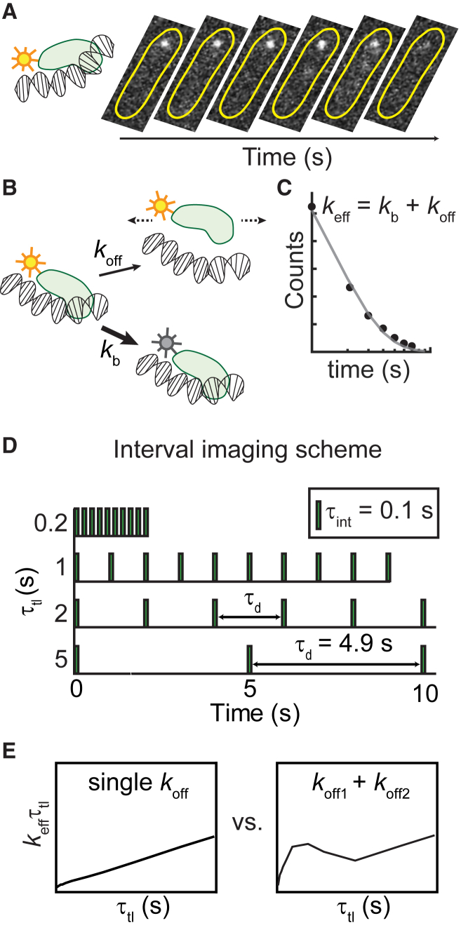
Compared to in vitro studies, live-cell investigations offer the key advantage of studying biochemical reactions at physiological conditions that can be difficult to reconstitute. Single-molecule live-cell imaging commonly relies on fluorescent proteins that are genetically fused to the protein of interest (Fig. 1 A; (18, 19, 20, 21, 22)). Tracking the fluorescence signal of thousands of molecules, one molecule at a time, enables the building of physical models from which physical parameters such as diffusion constants and detachment rates from DNA can be determined. Where detachment rates are concerned, the trajectory lengths of thousands of molecules are aligned to obtain a cumulative residence time distribution (CRTD). At the single-molecule level, the dissociation of a protein from its substrate is a stochastic process. This phenomenon can be adequately described as a two-state kinetic model with the interconversion of populations being modeled as a Poisson process. The resulting CRTD can be fit to exponential functions to obtain decay rates. In the case of a fluorescently tagged protein in which loss of fluorescence is attributable to either dissociation or photobleaching of the chromophore, the decay rate represents a combination of dissociation rates and photobleaching rate (Fig. 1, B and C; (23)).

Figure 1.

Experimental approach for characterizing kinetic heterogeneity of protein binding in live cells using single-molecule fluorescence imaging. (A) The protein of interest is tagged with a fluorescent protein. When the protein binds to the DNA substrate, its fluorescence signal appears as a diffraction-limited focus that can be tracked in real time. Subsequent dissociation results in the disappearance of the focus and a redistribution of the fluorescence signal throughout the cell. Yellow outlines illustrate the bacterial cell membrane. (B) The loss of fluorescence is attributable to either dissociation or photobleaching of the chromophore. (C) Cumulative residence time distribution (CRTD) is constructed from binding durations of thousands of molecules. Fitting the exponential function (Eq. 1) to CRTD yields an effective rate k_eff, which is the sum of off rate (k_off) of the protein of interest and photobleaching rate (k_b) of the fluorescent probe (23). (D) To deconvolute k_b and k_off, excitation and integration durations (τ_int) can be spaced with various dark intervals (τ_d). (E) Through exponential analyses, CRTDs obtained at various intervals result in k_effτ_tl plots, which are indicators of kinetic heterogeneity (23). A single kinetic population yields a straight line, whereas deviations from linear fits indicate the presence of a second kinetic subpopulation. For a single kinetic population, the slope is the off rate, and the y intercept is proportional to the photobleaching rate. To see this figure in color, go online.

Photobleaching, a result of fluorescent proteins being damaged upon exposure to excitation sources, leads to the loss of fluorescence signal (24). Under excitation conditions that guarantee good signal-to-background ratios, fluorescent proteins can only stay “on” for a few frames during continuous acquisitions. This limited visualization window reflects the “photon budget” (25). Thus, when photobleaching occurs faster than the dissociation process, lifetime measurements are limited by the photobleaching rate. To overcome this problem and extend the observation time, the observation time window can be expanded by temporally spacing the photon budget using stroboscopic imaging (26). In this method, a dark interval (τ_d) is inserted between integration time (τ_int), effectively scaling the observation time with a factor of τ_tl/τ_int (τ_tl = τ_int + τ_d). Instead of using one dark interval, Gebhardt and co-workers (23) developed an approach involving “time-lapse illumination with a fixed integration time, interspersed with dark periods of varying duration” in which fluorescence acquisitions are collected at a series of time-lapse intervals (Fig. 1 D; (23, 27)). This method has also been variously referred to as “time-lapse imaging” (28), “time-lapse illumination with different dark times” (29), “time-lapse imaging at multiple timescales” (30), and “stroboscopic single particle tracking PALM” (31). For the purpose of brevity and to distinguish from a time-lapse imaging mode with a single dark interval, we have adopted the term “interval imaging” in our lab (32). Briefly, the approach works as follows: first, several videos (each with a unique dark interval) are collected while keeping the photon budget constant (in practice, this is achieved by keeping the number of frames constant across all the videos). In cases in which the copy number of the tagged protein is high and single-molecule imaging conditions may be difficult to attain, the cellular fluorescence is first photobleached such that only single-molecule fluorescence is observable. Subsequently, using particle tracking algorithms that enable measurements of lifetimes of bound molecules within a specified localization radius, a CRTD can be compiled. Fitting the CRTDs to effective rates (k_eff), one can obtain the so-called k_effτ_tl plot, which is linear for monoexponential distributions (Fig. 1 E; (23)). In this case, because the photobleaching rate is maintained constant across all conditions, it can be read off from the intercept on the y axis. A population of molecules dissociating with a finite and measurable off rate manifests as a straight line, in which the slope reports on the off rate of the dissociation kinetics. A mixed population composed of species dissociating with multiple lifetimes manifests as a deviation from the linear fit (Fig. 1 E; (23)). Fitting the experimental data to a model describing mixed populations can then be used to extract the relative amplitudes and rates of the various populations. This power to deconvolute the photobleaching rate from multiple off rates has been successfully harnessed to dissect the kinetic heterogeneity of various DNA-binding proteins, including transcription factors and DNA replication and repair proteins in live cells (23, 27, 28, 29, 30, 31, 32, 33).

However, limitations arising from the practical implementation of this elegant method remain uncharacterized. In particular, we address the following questions: 1) What is the minimal number of observations needed to determine the binding lifetime of a species within a specified confidence; 2) for a given experimental setup, what is the dynamic range in binding lifetimes that can be detected; 3) how many populations can be resolved; and 4) what limits the ability to reliably resolve multiple populations? We consider four cases below to answer these questions. This study serves to provide a practical guide to realize the power as well as limitations of practical implementations of the interval imaging approach to measure intracellular binding kinetics of fluorescently tagged proteins.

Methods

Rationale and model

For an introduction to the method, we direct the reader to the seminal work by Gebhardt and co-workers who have developed and demonstrated the time-lapse imaging approach discussed here (23). Here, we first summarize the theoretical development to establish the context of the problem for this report. Consider a system containing “A” number of fluorescently tagged DNA-bound proteins, wherein the proteins dissociate from DNA with a single off rate (k_off). Upon exposure to excitation photon sources, the fluorescent proteins exhibit photobleaching with a rate k_b, resulting in the loss of fluorescence signal. Additionally, dissociation contributes to the loss of fluorescent foci as protein molecules move out of the localization radius. Because dissociation and photobleaching are independent and both are Poisson processes, the loss of observations as a function of time t can be described as follows (23):

$$f_1\left(t\right)=A\exp \left(-\left(k_{\text{b}}+k_{\text{off}}\right)t\right).$$ (1)

Observation times of genetically expressible fluorescent proteins are severely limited to the duration of a few acquisition frames because of photobleaching, which limits measurements of long-lived binding events (34). To extend observation times, the frame rate can be reduced by inserting a dark interval (τ_d) after a short integration time (τ_int). Scaling the photobleaching rate appropriately, Eq. 1 then becomes the following (23):

$$f_2\left(t\right)=A\exp \left(-\left(k_{\text{b}}{\mathit{\tau }}_{\text{int}}/{\mathit{\tau }}_{\text{tl}}+k_{\text{off}}\right)t\right),$$ (2)

where the time-lapse time τ_tl is the sum of τ_int and τ_d. The sum of two decay rates k_b and k_off can be approximated with an effective decay rate (k_eff) (23):

$$k_{\text{eff}}=k_{\text{b}}{\mathit{\tau }}_{\text{int}}/{\mathit{\tau }}_{\text{tl}}+k_{\text{off }}.$$ (3)

The rearrangement of Eq. 3 yields the following (23):

$$k_{\text{eff}}{\mathit{\tau }}_{\text{tl}}=k_{\text{b}}{\mathit{\tau }}_{\mathrm{int}}+k_{\text{off}}{\mathit{\tau }}_{\text{tl}}.$$ (4)

As k_bτ_int is maintained constant at a certain imaging condition, k_effτ_tl increases linearly with τ_tl, with the coefficient (slope) k_off.

In systems with two subpopulations each dissociating at different rates k_off1 and k_off2, Eq. 2 then becomes the following (23):

$$f_3\left(t\right)=A\left(B\text{exp}\left(-\left(k_{\text{b}}{\mathit{\tau }}_{\text{int}}/{\mathit{\tau }}_{\text{tl}}+k_{\text{off}1}\right)t\right)+\left(1-B\right)\text{exp}\left(-\left(k_{\text{b}}{\mathit{\tau }}_{\text{int}}/{\mathit{\tau }}_{\text{tl}}+k_{\text{off}2}\right)t\right)\right),$$ (5)

where B (0 < B < 1) and (1 – B) are the amplitudes of k_off1 and k_off2 subpopulations, respectively.

Similarly, a system with three kinetic subpopulations can be described by the following (29):

$$f_4\left(t\right)=A\left(B_1\text{exp}\left(-\left(k_{\text{b}}{\mathit{\tau }}_{\text{int}}/{\mathit{\tau }}_{\text{tl}}+k_{\text{off}1}\right)t\right)+B_2\text{exp}\left(-\left(k_{\text{b}}{\mathit{\tau }}_{\text{int}}/{\mathit{\tau }}_{\text{tl}}+k_{\text{off}2}\right)t\right)+\left(1-B_1-B_2\right)\text{exp}\left(-\left(k_{\text{b}}{\mathit{\tau }}_{\text{int}}/{\mathit{\tau }}_{\text{tl}}+k_{\text{off}3}\right)t\right)\right),$$ (6)

where B₁, B₂ (0 < B₁, B₂ < 1 and B₁ + B₂ < 1), and (1 – B₁ – B₂) represent the amplitudes of k_off1, k_off2, and k_off3 subpopulations, respectively.

Experimental considerations

The specifics of the experimental setup for different model organisms should be tailored to requirements for the respective system. However, to provide the reader with a starting point, we describe the experimental configuration used in our lab to measure binding lifetimes of DNA repair proteins labeled with the fluorescent protein, YPet, in the model organism Escherichia coli (see Fig. S1; (32)). Bacterial cells (MG1655 cells carrying mfd-YPet in place of mfd) in the early exponential phase are loaded into a custom-built flow cell made up a glass coverslip and a quartz top. The bottom coverslip is functionalized with (3-Aminopropyl)triethoxysilane (Alfa Aesar, Haverhill, MA) to facilitate cell adhesion to the surface of the coverslip. The temperature of the flow cell is kept constant at 30°C. Cells are supplied with aerated rich-defined media (EZ rich-defined medium supplemented with glucose; Teknova, Hollister) to maintain fast growth. YPet is excited with 514-nm laser (Sapphire LP laser; Coherent, Santa Clara, CA) in near-total internal reflection fluorescence configuration (35) at a power density of 71 W/cm² (measured directly above the inverted objective). Fluorescent signal is recorded using an electron-multiplying-CCD camera (Photometrics Evolve; Teledyne Photometrics, Tucson, AZ), with an electron-multiplying gain of 1000. The camera exposure time is 0.1 s, and time-lapse imaging is acquired with a 10-s τ_tl set (Table S2). Typically, a time-lapse imaging experiment lasts 3–5 h and in generally 4–10 experiments are required to obtain more than 1000 binding events at each τ_tl.

Resolution of binding events in bacterial cells expressing copy numbers of fluorescent proteins in excess of ∼20 copies per cell is challenging because of the limitations of particle tracking algorithms to resolve closely spaced foci. Further, distinguishing bound molecules from freely diffusive molecules in the cytosol is also challenging when copy numbers are high. In this case, to enable the reliable observation of single molecules, cells are exposed to continuous illumination such that the majority of the emitters are darkened or photobleached, and only stochastically reactivated emitters are observed in single-molecule imaging conditions (36).

This setup allows us to unambiguously detect single-molecule foci using a relative signal-to-background ratio between six and eight. Foci detected in at least two consecutive frames within a 300-nm (three pixels) radius are defined as a binding event. For each τ_tl, all binding events are combined, and bootstrapping analysis is performed by randomly selecting with replacements 80% of all binding events. CRTDs are constructed from bootstrapped samples and are fit to exponential models to obtain k_effτ_tl plots as well as k_b and τ.

Simulating concurrent dissociation and photobleaching

To maintain full control of the kinetic variables, we chose to perform simulations of the experiment. Simulations of exponential distributions and curve-fitting were performed with a custom-written program in MATLAB (The MathWorks, Natick, MA). We simulated exponential distributions (Eqs. 2, 5, and 6) using the exprnd function in MATLAB (Supporting Materials and Methods). This function generates exponentially distributed random numbers with a specified decay constant. Here, each number returned by exprnd function represents the lifetime of a simulated “trajectory.” For the purposes of this work, we have not accounted for blinking of bound molecules that may yield prematurely truncated binding events. Accommodation of such a feature will require reasonable estimates of FP blinking under the conditions of the experiment that will be unique to the fluorescent probe used. To simulate a subpopulation of molecules dissociating with a specified off rate, a set of trajectories was generated and binned to produce histograms with 10 bins whose edges correspond to frame times (integer multiples of τ_tl). The exprnd function was iterated until the counts of the first bin exceeded the number of binding events in that subpopulation (typically between three and six iterations, see Fig. S2). To simulate experiments in which multiple subpopulations are present, each subpopulation was simulated in defined proportions, and all trajectories were pooled together. Finally, to generate the CRTDs, we rejected molecules in the first bin (0 to τ_tl) and only carried forward observations from τ_tl to 10τ_tl to the next step in accordance with our definition of a binding event (or trajectories) (i.e., the observation must be present in two consecutive frames).

To simulate uncertainty in each simulation sample, 10 rounds of bootstrapping were performed, each involved in randomly sampling 80% of the simulated population. Next, fitting was performed on each bootstrapped CRTD (henceforth referred simply as CRTDs). First, the CRTD at each τ_tl was fit to a monoexponential model to obtain k_eff (Eqs. 2 and 3; Fig. 1 C). These values for k_eff, corresponding to the number of τ_tl, were then used to construct the k_effτ_tl plot. Error bands in these plots represent SDs from 10 bootstrapped samples.

Second, the CRTDs for all τ_tl were fit to objective functions based on Eqs. 2, 5, and 6 (global fitting, see Supporting Materials and Methods). The list of parameters, initial conditions, bound constraints, termination criteria, and algorithm is presented in Table S1. Throughout the article, A was set as a local parameter to mimic experimental conditions in which counts may be different across τ_tl, even though this often leads to less accurate results compared to when A was set as a global parameter (Fig. S3, B and C).

For each simulation, outcomes from globally fitting the 10 bootstrapped CRTDs were averaged and reported. To determine uncertainty in the estimate, we repeated the simulation 100 times. The SDs of the binding lifetime (σ_τ) from 100 simulations using the same conditions was calculated according to Eq. 7:

$${\text{σ}}_{\text{τ}}={\left(\sum _{i=1}^{100}{\left({\mathit{\tau }}_i-\langle \mathit{\tau }\rangle \right)}^2/100\right)}^{1/2},$$ (7)

where <τ> denotes the true binding lifetime, which is calculated by 1/<k_off>.

Unless otherwise stated, k_bτ_int was fixed at 0.7 to mimic experimental values obtained in our published work (32). Four sets of τ_tl were used: 10-s τ_tl, 100-s τ_tl, and the three and five τ_tl sets (Table S2).

Results

Influence of experimental sample size on uncertainty of the estimate of the binding lifetime

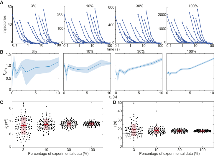
First, we set out to investigate whether the size of the experimental data set influences the uncertainty in the error estimate of the outcomes from global fitting, such as the binding lifetime τ and photobleaching rate k_b. This can be achieved by randomly selecting a fraction of experimental data (3–30%) at each τ_tl, followed by bootstrapping and global fitting. Toward this goal, we revisited published data from our laboratory in which interval imaging was used to determine the dissociation kinetics of the transcription-repair coupling factor Mfd from DNA in live E. coli (32). The entire data set (100%) contains between 1000 and 2000 trajectories (counts lasting at least two frames) at each τ_tl (Fig. 2 A, right-most panel). Representative CRTDs after subsampling the experimental data set (3, 10, and 30%) at each τ_tl are shown in (Fig. 2 A). Although the k_effτ_tl plot derived from the whole data set resembles a straight line, deviations from linear fits in k_effτ_tl plots can be seen when only a subset of experimental data was used (Fig. 2 B).

Figure 2.

Determination of the photobleaching rate and binding lifetime from subsampling experimental data. (A) Representative CRTDs when only 3, 10, or 30% of experimental trajectories were randomly selected. Counts can be approximated as y intercepts of exponential fits of CRTDs. The CRTD from the full data set (right-most panel) is reproduced from (32). (B) Shown are k_effτ_tl plots of the corresponding CRTDs (above). Shaded error bands are SDs from 10 bootstrapped samples. (C) Scatter plots show distributions of k_b obtained using the global fitting of 100 subsets of the experimental data at the indicated fraction. Each point represents the average of results from 10 bootstrapped samples. (D) Scatter plots show distributions of τ obtained using the global fitting of 100 subsets of the experimental data at the indicated fraction. Similarly, each point represents the average of results from 10 bootstrapped samples. Bars and boxes represent means and SDs of the fitting outcomes of 100 subsets of the data set, respectively. The experimentally measured value of τ = 17.9 ± 0.9 s for the entire data set is reproduced from (32). To see this figure in color, go online.

To determine the uncertainties in k_b and τ as a result of undersampling, we repeated the subsampling 100 times, and k_b and τ values were obtained from global fitting using Eq. 2 (Fig. 2, C and D). Here, uncertainties in the estimates of k_b and τ are smallest when the entire data set is used (2 and 5%, respectively, Fig. 2, C and D) and, as expected, increase with decreasing number of counts (Fig. 2, C and D). For k_b, uncertainties increase from 3 to 10% as the percentage of experimental data drop from 30 to 3%, whereas uncertainties in determining binding lifetimes increase from 8 to 35% (Fig. 2, C and D).

Fitting individual CRTD to a monoexponential model to obtain k_effτ_tl plots has been suggested to be used as a guide to determine kinetic heterogeneity (23). Our analysis demonstrates that deviation from linear fits in the k_effτ_tl plots can potentially simply reflect undersampling. Because deviations from linear fits in k_effτ_tl plots can also be used to guide the choice of bi- and triexponential models (23), a fundamental question that faces users is what governs the choice of exponential model? What is the minimal size of data, for which a multiexponential model is appropriate for consideration? Are deviations in the k_effτ_tl plots reliable indicators for the choice of model? To explore these questions in greater detail, we chose to perform simulations that permit us to retain full control of the model parameters and overcome practical limitations of generating large data sets from microscopy experiments.

Case I: Influence of the size of the data set on the measured lifetime for a single dissociating species

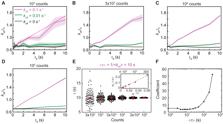
We first explored the relationship between the number of counts (n) at each τ_tl and uncertainties in estimates of binding lifetimes from monoexponential distributions. To this end, we simulated a population of molecules dissociating with k_off of 0.1 s⁻¹, corresponding to a binding lifetime <τ> of 10 s, and photobleaching rate k_b of 7 s⁻¹ (see Methods). Whereas τ_int was constant at 0.1 s, τ_tl was varied from 0.1 to 10 s (Table S2). These values of k_b, <τ>, τ_int, and τ_tl were initially chosen to closely match experimental values used in our published work (see Fig. 2; (32)). The theoretical k_effτ_tl plot is shown as the dashed line (Fig. 3 A). At n = 1 × 10³ observations (Fig. 3 A), the k_effτ_tl plot deviates noticeably from the theoretical line. However, as n increases, the error bands reduce, and the plots closely resemble straight lines (Fig. 3, B–D). At 1 × 10⁵ observations, linearly fitting the k_effτ_tl plot (Fig. 3 D) yielded a slope of 0.1 and y intercept of 0.6992, reflecting the specified k_off (0.1 s⁻¹) and k_bτ_int (0.7). As expected, monoexponential distributions with the same k_bτ_int but smaller off rate (k_off = 0.01 s⁻¹) or without off rate (k_off = 0 s⁻¹) yielded lines with a smaller slope (Fig. 3, A–D) or essentially flat lines (Fig. 3, A–D).

Figure 3.

Determination of binding lifetimes from monoexponential distributions. (A–D) Shown are k_effτ_tl plots of monoexponential distributions with k_bτ_int of 0.7 and k_off of 0.1 s⁻¹, 0.01 s⁻¹, or 0 s⁻¹. (A–D) reflect k_effτ_tl plots obtained from simulations containing a number of observations (n) equaling (A) 1 × 10³, (B) 3 × 10³, (C) 1 × 10⁴, or (D) 1 × 10⁵ counts in the first bin (see Methods). (A) Dashed lines correspond to theoretical k_effτ_tl plots at the specified k_off values. Shaded error bands are SDs from 10 bootstrapped samples. (E) Scatter plots show distributions of τ obtained using the global fitting from 100 simulated samples for each n value. Bars represent the mean values. (Inset) The relative error in determining τ (σ_τ/<τ>) reduces with n^−1/2 for increasing n. Dashed line is the linear fit to six data points. (F) Shown is the coefficient in function of σ_τ/<τ> versus n^−1/2 at various <τ>. The sharp increase in coefficients for <τ> larger than 50 s indicates larger uncertainties in measuring slow processes when the maximal τ_tl is limited to 10 s. To see this figure in color, go online.

To characterize the uncertainty (SD, σ_τ) in the estimate of the binding lifetime, we repeated the simulation 100 times for each value of n and determined τ using global fitting (Fig. 3 E). As expected for shot noise (37), the relative error σ_τ/<τ> is proportional to the inverse of the square root of n with a coefficient of 3.8 (Fig. 3 E, inset). Importantly, the coefficient fluctuates between 3.7 and 5.7 for <τ> ≤50 s but rises sharply for <τ> >50 s (Fig. 3 F). This result demonstrates that the uncertainty in estimating the lifetime of long-lived binding events becomes arbitrarily large when the extended lifetime of the fluorophore (by introduction of τ_d) becomes comparable to the binding lifetime. In principle, this limit can be readily overcome by simply selecting larger τ_tl values; indeed, simulations of monoexponential distributions of long-lived binding events (τ = 100 s) indicated that σ_τ is lower at lower values of n when τ_tl is extended to 100 s, compared to 10 s (Fig. S3).

Therefore, we propose that accurate measurements of lifetime of long-lived binding events require significant increases in either the number of observations (n) or the length of τ_tl for a fixed photobleaching rate. However, it should be noted that extension of τ_tl up to 100 s may not be experimentally feasible for all systems. In our work involving bacterial live-cell imaging in rich media, cell growth and division on the timescale of imaging limit the tracking binding events lasting on the timescale of tens of minutes. Practical limitations imposed by the model organism, growth conditions, and choice of fluorescent protein dictate optimal experimental design.

Further, we anticipated that the photobleaching rate also contributes to σ_τ because faster photobleaching reduces observation times. To examine the effect of k_bτ_int, we performed a comprehensive set of simulations with the 10-s τ_tl set (Table S2) and k_bτ_int varying from 0.007 to 2.1 (k_b from 0.07 to 70 s⁻¹ and τ_int from 0.01 to 0.1 s). We obtained the relationship between σ_τ/τ, n, and k_bτ_int as in Eq. 8:

$$\frac{{\sigma }_{\mathit{\tau }}}{\mathit{\tau }}=\frac{{\left(2.7379k_{\text{b}}{\mathit{\tau }}_{\text{int}}\right)}^2}{n^{1/2}}.$$ (8)

This formula describes the lower bound of errors as other sources of practical errors, such as localization uncertainties and experimental variations, have not been considered. The minimal number of observations required to determine τ (<τ> ≤ 50 s) with a given uncertainty is therefore as follows:

$$n={\left(\mathit{\tau }/{\sigma }_{\mathit{\tau }}\right)}^2\times {\left(2.7379k_b{\mathit{\tau }}_{\text{int}}\right)}^4.$$ (9)

For example, when k_bτ_int is 0.7, the number of observations required to achieve a relative error of 10% in the estimate of τ (where <τ> ≤ 50 s) is ∼1350 (see Fig. 3 E). This equation also highlights the importance of using fluorophores with high photostability; a twofold increase in k_b needs to be compensated by a 16-fold increase in n.

Case II: Detection of two species with resolvable lifetimes

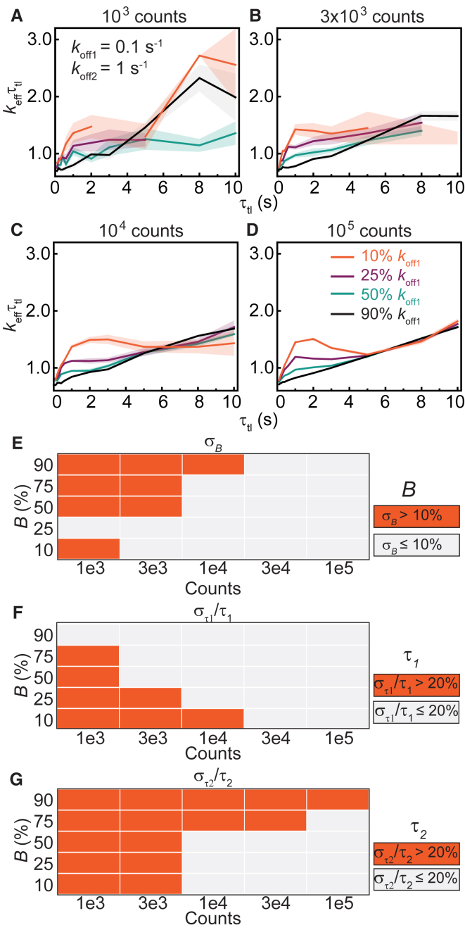
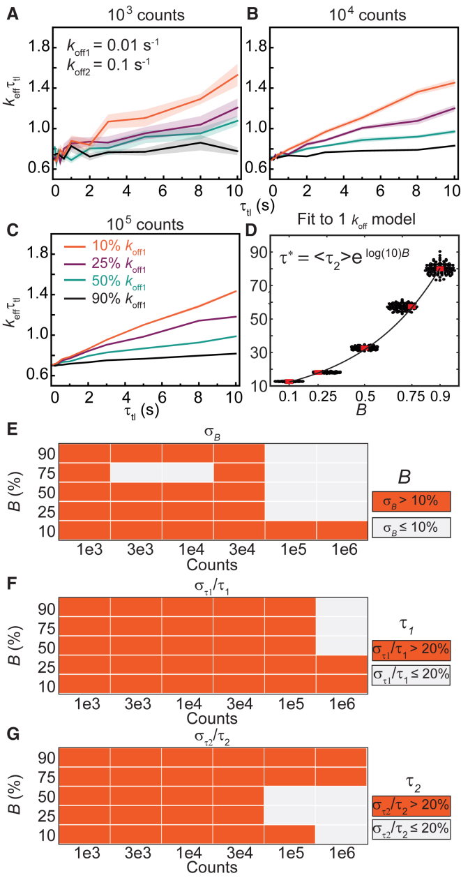
Next, we examined the situation in which a second kinetic subpopulation is present in the system. A second population with a faster off rate yields k_effτ_tl plots that deviate from straight lines (23). However, as we demonstrate, deviations can also be a result of shot noise at low n (see Figs. 2 B and 3, A–D). To identify the minimal n at which one can determine with a specified confidence that a biexponential model is appropriate, we simulated CRTDs using Eq. 5. First, we performed simulations with off rates that are an order of magnitude apart: k_off1 = 0.1 s⁻¹ (intermediate rate) and k_off2 = 1 s⁻¹ (fast rate). The amplitude B of the intermediate dissociating population was varied from 10 to 90% (Fig. 4).

Figure 4.

Determination of binding lifetimes and amplitudes from biexponential distributions with an intermediate rate (k_off1) and a fast rate (k_off2 = 10 k_off1). (A–D) Shown are k_effτ_tl plots of biexponential distributions with k_bτ_int of 0.7, k_off1 and k_off2 of 0.1 and 1.0 s⁻¹, respectively, with (A) 1 × 10³, (B) 3 × 10³, (C) 1 × 10⁴, or (D) 1 × 10⁵ observations. The amplitude of k_off1 (B) is 10%, 25%, 50%, or 90%. Shaded error bars are SDs from 10 bootstrapped samples. (E–G) Heatmaps show errors in estimates of B, τ₁, and τ₂ obtained using the global fitting of 100 simulated distributions for each n value (see Fig. S4 for distributions). To see this figure in color, go online.

When the majority of the population dissociates with the intermediate rate k_off1 (B = 90%), the k_effτ_tl plots resemble those of monoexponential distribution with the single k_off of 0.1 s⁻¹ (compare Fig. 4, A–D, and Fig. 3, A–D). As before, increasing the number of observations significantly improved the quality of the k_effτ_tl plots (Fig. 4, A–D). These simulations reveal that a short-lived second subpopulation does not manifest as a visible feature in the k_effτ_tl plots when it is present only to the extent of 10% in the observations. To examine if the two populations could be resolved with global fitting using the biexponential model, we determined binding lifetimes and amplitudes from 100 simulations (Fig. S4). Unsurprisingly, we found that the accuracies and precisions of determining B, τ₁, and τ₂ increase with n. Although estimation of τ₁ is robust (Fig. 4 F; Fig. S4 B), global fitting of CRTDs to the biexponential model at low counts suffers from a bias toward the fast-dissociating subpopulation, with its amplitude being overestimated and τ₂ being underestimated (Fig. 4, E and G; Fig. S4, A and C). This bias is observed to a lesser extent when k_off1 is present at 75 or 50% (Fig. 4, E–G; Fig. S4).

As the amplitude of the fast-dissociating subpopulation increased (B equal to 25 or 10%), fewer observations were found at long intervals. Insufficient counts resulted in missing data points at these τ_tl (τ_tl ≥ 5 s) in k_effτ_tl plots at low counts (1 × 10³ and 3 × 10³, Fig. 4, A and B). However, the k_effτ_tl plots extended to the full τ_tl range of 10 s when n increases to 1 × 10⁴ and 1 × 10⁵ (Fig. 4, C and D). As expected, deviations from straight lines were found in the 0–5 s regime, reflecting the presence of the fast-dissociating subpopulation. Because contributions from the fast-dissociating subpopulation drop sharply at long timescales, the k_effτ_tl plots converge to the straight line exhibited by monoexponential distributions with k_off1 (Fig. 4, C and D). Further analysis by integrating the area under the peaks in the 0 to 5 s region shows the area increases exponentially with the amplitude of the fast-dissociating subpopulation (Fig. S5). When the fast-dissociating subpopulation represents the majority, the accuracy and precision in determining B, τ₁, and τ₂ also increase with n (Fig. 4, E–G; Fig. S4).

Based on the observation that accurate measurements of long-lived binding events require the extension of τ_tl to greater than 10 s, we anticipated that resolving two kinetic subpopulations (one with a slow rate (k_off1 of 0.01 s⁻¹; <τ₁> = 100 s) and an intermediate rate (k_off2 of 0.1 s⁻¹; <τ₂> = 10 s)) is challenging when the largest τ_tl is 10 s. Consistent with this, the k_effτ_tl plots in the 0–10 s range appear linear (Fig. 5, A–C), resembling those of monoexponential distributions. Hence, we attempted to fit the CRTDs at 1 × 10⁵ counts to a monoexponential model (Eq. 2), yielding apparent binding lifetimes (τ^∗) that lie between <τ₁> and <τ₂> (Fig. 5 D). Fitting mean τ^∗ versus B to exponential function results in Eq. 10:

$${\mathit{\tau }}^{\ast }=\langle {\mathit{\tau }}_2\rangle e^{log\left(\langle {\mathit{\tau }}_1\rangle /\langle {\mathit{\tau }}_2\rangle \right)B}.$$ (10)

Thus, B can be derived from τ^∗, where <τ₁> and <τ₂ > are known.

Figure 5.

Determination of binding lifetimes and amplitudes from biexponential distributions with a slow rate (k_off1) and an intermediate rate (k_off2 = 10k_off1). (A–C) Shown are k_effτ_tl plots of biexponential distributions with k_bτ_int of 0.7, k_off1 and k_off2 of 0.01 and 0.1 s⁻¹, respectively, with (A) 1 × 10³, (B) 1 × 10⁴, or (C) 1 × 10⁵ observations. The amplitude of k_off1 (B) is 10%, 25%, 50%, or 90%. Shaded error bars are SDs from 10 bootstrapped samples. (D) Scatter plots show a distribution of apparent τ (τ^∗) obtained from the fitting of 100 simulated biexponential distributions at a specified B and 1 × 10⁵ counts to a monoexponential model. Line is the exponential fit between the average of τ^∗ (represented by bars) and B. (E–G) Heatmaps show errors in estimates of B, τ₁, and τ₂ obtained using the global fitting of 100 simulated distributions for each n value (see Fig. S6 for distributions). To see this figure in color, go online.

From the simulations, fitting the CRTDs with n less than 3 × 10⁴ to the biexponential model yields unreliable results (Fig. 5, E–G; Fig. S6). Across various amplitudes of k_off1, the species with lifetime τ₁ is often underestimated and corresponds to τ^∗ at that amplitude (compare Fig. 5 F to Fig. 5 D). Similarly, τ₂ is also underestimated, but eventually approaches <τ₂> of 10 s when n reached 1 × 10⁶ counts, and the amplitude of k_off2 subpopulation is more than 25% (Fig. 5 G).

On the other hand, when the above distributions were simulated using the 100-s τ_tl set, deviations from straight lines in k_effτ_tl plots were observed in the 0–30 s regime and when B is smaller than 75% (Fig. S7 A). In this case, as expected, accuracies in determining B, τ₁, and τ₂ follow the same trends as discussed in Fig. 4 (Fig. S7, B–D).

Case III: Detection of two species with closely matched lifetimes

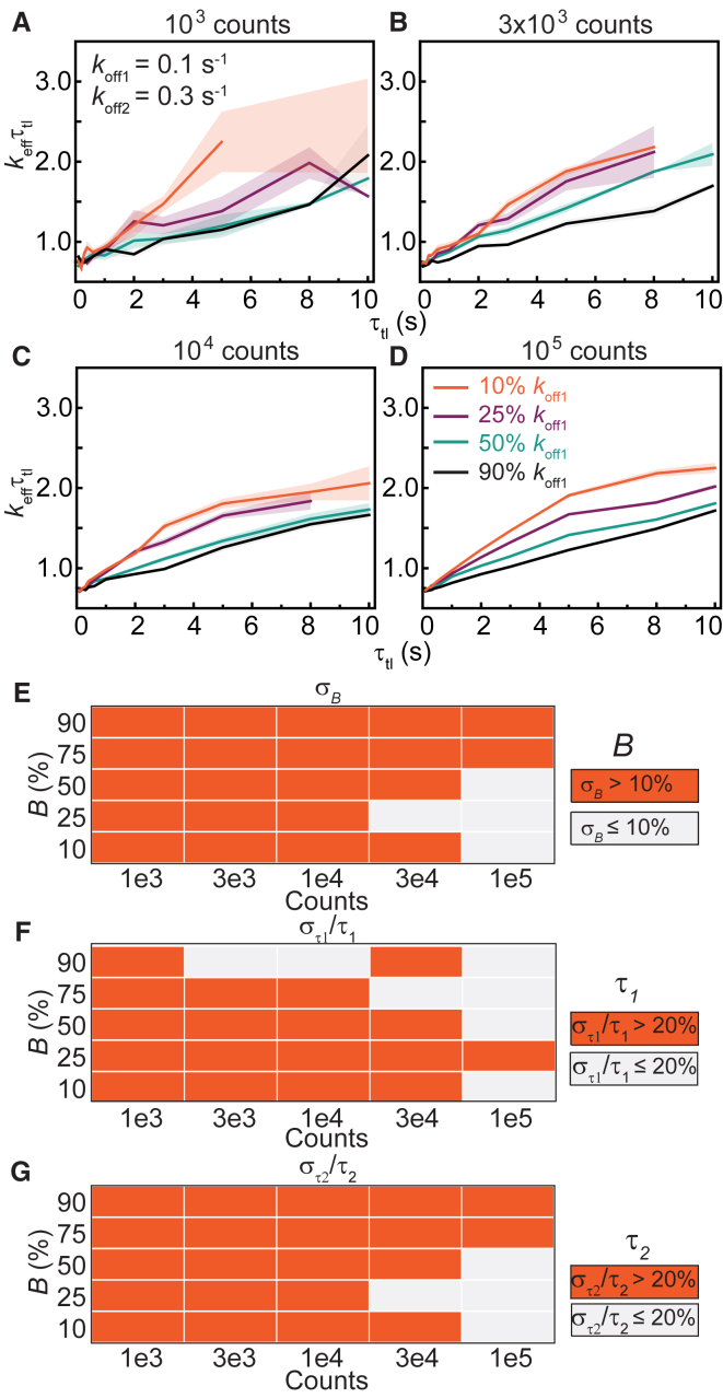
We anticipated that resolution limits inherent to exponential analyses (34) would reduce the ability to resolve closely-spaced rates. To test this hypothesis, we simulated biexponential distributions with rates that are only threefold apart: an intermediate rate k_off1 of 0.1 s⁻¹ and a fast rate k_off2 of 0.3 s⁻¹. Under conditions that yield sufficient observations at long intervals (n ≥ 1 × 10⁴), examination of the k_effτ_tl plots often fails to identify the presence of multiple subpopulations in the form of deviation from straight lines (Fig. 6, A–D). Only when the fast rate is present at 90% can deviations be observed in the form of a broad convex spanning from 0 to 10 s (Fig. 6, C and D). Fitting to Eq. 5 yields unreliable results for B and τ₂ for n ≤ 1 × 10⁴ (Fig. 6, E and G; Fig. S8, A and C), whereas the accuracy in determining τ₁ requires 3 × 10³ observations or <B> to be larger than 25% (Fig. 6 F; Fig. S8 B). Fitting CRTDs at low counts (n ≤ 1 × 10⁴) to the biexponential model should be avoided as one often obtains two kinetics subpopulations with artificially enhanced rate separation and substantial amplitudes, regardless of the true amplitudes (Fig. 6, E–G; Fig. S8).

Figure 6.

Determination of binding lifetimes and amplitudes from biexponential distributions with closely spaced rates (k_off2 = 3k_off1). (A–D) Shown are k_effτ_tl plots of biexponential distributions with k_bτ_int of 0.7, k_off1 and k_off2 of 0.1 and 0.3 s⁻¹, respectively, with (A) 1 × 10³, (B) 3 × 10³, (C) 1 × 10⁴, or (D) 1 × 10⁵ observations. The amplitude of k_off1 (B) is 10%, 25%, 50%, or 90%. Shaded error bars are SDs from 10 bootstrapped samples. (E–G) Heatmaps show errors in estimates of B, τ₁, and τ₂ obtained using the global fitting of 100 simulated distributions for each n value (see Fig. S8 for distributions). To see this figure in color, go online.

Case IV: Detection of three species

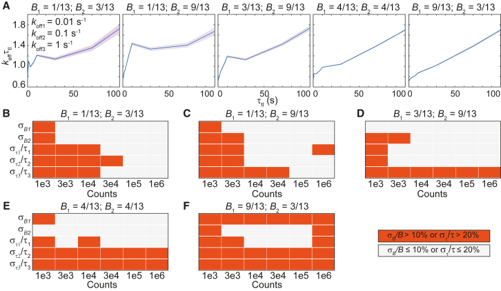
The resolution limit as well as dynamic range limit that we demonstrated above raises the question if triexponential distributions can be faithfully resolved under the specified experimental condition (ranges of τ_tl and n). To address this issue, we simulated triexponential distributions (Eq. 6) with off rates spanning two orders of magnitude (0.01, 0.1, and 1 s⁻¹), using the 100-s τ_tl set. The diversity in k_effτ_tl plots obtained by varying B₁ and B₂ is illustrated in Fig. 7 A. Three kinetic subpopulations are apparent when B₁ is a third of B₂ and B₂ in turn is a third of B₃ (1 – B₁ – B₂). We further characterized uncertainties in amplitudes and binding lifetimes obtained using global fitting to the triexponential model (Methods). In general, accuracy in determining the amplitudes and lifetimes improves with increasing n (Fig. 7, B–F; Fig. S9). However, when the slowly dissociating subpopulation dominates (B₁ = 9/13), increasing n does not yield more accurate estimates. As in the case of the biexponential simulations, we observed consistent biases toward faster binding lifetimes (Fig. S9).

Figure 7.

Determination of binding lifetimes and amplitudes from triexponential distributions with a slow rate (k_off1), an intermediate rate (k_off2 = 10k_off1), and a fast rate (k_off3 = 10k_off2), using the 100-s τ_tl set. From left to right, five panels in each row correspond to different amplitudes of each subpopulation (displayed on top). (A) Shown are k_effτ_tl plots of triexponential distributions with k_bτ_int of 0.7 and k_off1, k_off2, and k_off3 of 0.01, 0.1, and 1 s⁻¹, respectively, with 1 × 10⁶ observations. Shaded error bands are SDs from 10 bootstrapped samples. (B–F) Heatmaps show errors in estimates of B₁, B₂, τ₁, τ₂, and τ₃ obtained using the global fitting of 100 simulated distributions at various preset values of B₁ and B₂ (see Fig. S9 for distributions). To see this figure in color, go online.

The choice of τ_tl

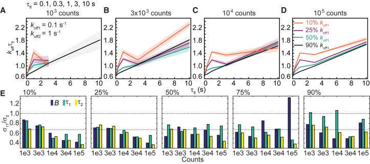
Given a finite amount of experimental time, should experimenters collect data with more τ_tl values (increase N_interval), or should we obtain more observations (increase n) with a set containing fewer τ_tl values? To identify the optimum choice of τ_tl, we simulated biexponential distributions with an intermediate rate (k_off1 = 0.1 s⁻¹) and a fast rate (k_off2 = 1 s⁻¹) using a τ_tl set containing either three (N₃) or five (N₅) τ_tl values, ranging from 0.1 to 10 s (Table S2). Because fitting outcomes are unreliable in the three τ_tl set (compare Fig. S10 to Fig. S11), we decided to examine the simulations with the five τ_tl set further. These simulations yielded k_effτ_tl plots that closely resemble those in Fig. 4 (see Fig. 8, A–D), and similarly, deviations from straight lines are also reliable indicators of kinetic heterogeneity when B is less than 90%. As expected, estimates of B, τ₁, and τ₂ are more accurate with larger n (Fig. S10).

Figure 8.

Determination of binding lifetimes and amplitudes from biexponential distributions using a τ_tl set containing five τ_tl values (Table S2), an intermediate rate (k_off1 = 0.1 s⁻¹), and a fast rate (k_off2 = 1 s⁻¹). (A–D) Shown are k_effτ_tl plots of biexponential distributions with (A) 1 × 10³, (B) 3 × 10³, (C) 1 × 10⁴ or (D) 1 × 10⁵ observations. The amplitude of k_off1 (B) is 10%, 25%, 50%, or 90%. Shaded error bands are SDs from 10 bootstrapped samples. (E) Bar plots show ratios of error estimates obtained from simulations with 11 and 5 τ_tl values at the same n. To see this figure in color, go online.

Comparing the simulations using the five τ_tl and the 10-s τ_tl (11 τ_tl values) sets for the same n, errors of estimates are almost always smaller in simulated distributions with the 10-s τ_tl set (σ₁₁/σ₅ < 1, see Fig. 8 E). By extension of Eq. 8, error ratios (σ₁₁/σ₅) smaller than 1/√(11/5) or 0.67 indicate the benefit of increasing N_interval outweighs the benefit of increasing n with the five τ_tl set, whereas error ratios larger than 0.67 represent redundancy in τ_tl. Redundancy in τ_tl was observed in some cases when the intermediate dissociating subpopulation is the majority (B between 75 and 90%) (Fig. 8 E). However, when the majority dissociates with the fast rate (B between 10 and 50%), the benefit of sampling with more τ_tl is clear (σ₁₁/σ₅ < 0.67), especially with n ≥ 1 × 10⁴. Thus, we concluded the net benefit of increasing N_interval is greater than increasing the number of counts with a set of fewer τ_tl values.

Discussion

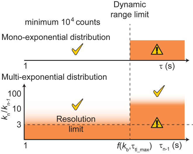
In this work, we used experimental and simulated data to explore the influence of shot noise, resolution limit, and dynamic range limit on resolving multiple kinetic subpopulations in single-molecule time-lapse imaging experiments (Fig. 9). Within the dynamic range and resolution limit, the determination of binding lifetimes and amplitudes in monoexponential and multiexponential distributions are reliable in general, especially with at least 1 × 10⁴ counts.

Figure 9.

Dynamic range and resolution limits in resolving multiple populations using the time-lapse imaging technique with photobleaching-prone fluorescent probes. Dynamic range limit is a function of the photobleaching rate (k_b) and the maximal τ_tl (τ_{tl_max}) used in experimental conditions. τ_n−1 is the longest binding lifetime in a multiexponential distribution within pairs of off rates k_n and k_n−1. Shaded zones indicate conditions in which errors in estimates of τ and the amplitude are high. To see this figure in color, go online.

As showed in Eq. 8, the relative error in τ determination scales with the square of k_bτ_int and the inverse square root of n. This emphasizes the importance of choosing imaging conditions to minimize k_bτ_int as a twofold increase in k_bτ_int needs to be compensated by a 16-fold increase in n. A balance has to be struck here to ensure good signal-to-background ratio, a prerequisite for reliable particle tracking. These findings also highlight the importance of developing and using fluorophores with higher photostability and brightness for live-cell applications as these would greatly reduce uncertainties in measurements. In practice, the choice of fluorescent protein should be made with great care because fluorescent proteins often exhibit undesirable properties that limit their utility (38, 39, 40, 41, 42).

Errors obtained from repeating the experiments can be an underestimation compared to inherent errors conferred by shot noise when fitting is ill conditioned (43), which is often the case when minimizing using multiobjective functions (44). Therefore, reports of binding lifetime measurements using these time-lapse imaging approaches should clearly state k_bτ_int from fitting and n from experimental data. This would enable a theoretical error estimation of τ and avoid the overinterpretation of experimental results.

We found k_effτ_tl plots useful for guiding the fitting model when the number of counts is sufficiently large (more than 1 × 10⁴) as deviations from straight lines faithfully reflect heterogeneity in binding kinetics. The reverse is not necessarily true. Good linear fits, seen at large n values, can reflect one of the following three scenarios: 1) the absence of multiple populations, 2) subpopulations with off rates that are within the resolution limit, or 3) subpopulations in which the off rate of one population lies beyond the dynamic range. This dynamic range is determined by the photobleaching rate and the maximal τ_tl used in the experiment. When the monoexponential model is used to fit those data, an apparent binding lifetime τ^∗, whose value lies between the two true binding lifetimes, is obtained. Although suboptimal, τ^∗ depends on the proportion of molecules in each kinetic subpopulation; a larger presence of the fast-dissociating subpopulation yields smaller τ^∗. This in turn can report on a change in binding kinetics when the biology is manipulable—for instance, with binding partners or drugs.

Can statistical information such as reduced χ² be used to decide the model that best describes the data? Computing these criteria requires the determination of the degree of freedom, which still needs to be analytically derived for the nonlinear models used in this method (45, 46, 47, 48). Instead of using statistical criteria, the selection of the fitting model using k_effτ_tl plot can be complemented with experimental design. For example, in a case in which a biexponential model is invoked, it might be tempting to attribute subpopulations to molecules performing certain activities, such as the binding of DNA repair proteins to a damaged or nondamaged substrate. These hypotheses can be tested using structure-function mutants in which one or few catalytic activities are inhibited, hence yielding predictable changes in k_effτ_tl plots and fitting results. Finally, where possible, we recommend approaches that utilize multiple experimental designs to reproducibly observe or enrich the hypothesized populations.

Software

Our algorithms are freely available as open source MATLAB codes from https://github.com/hanngocho/off-rate-simulation.

Author Contributions

H.N.H., H.G., and A.M.v.O. designed research. H.N.H. wrote the codes, conducted the simulations, and wrote the first draft. D.Z. contributed to the codes, with support from J.K. H.G. and A.M.v.O. revised the manuscript and supervised research.

Editor: Gijs Wuite.

References

- 1.Lu H.P., Xun L., Xie X.S. Single-molecule enzymatic dynamics. Science. 1998;282:1877–1882. doi: 10.1126/science.282.5395.1877. [DOI] [PubMed] [Google Scholar]
- 2.Xie X.S. Single-molecule approach to dispersed kinetics and dynamic disorder: probing conformational fluctuation and enzymatic dynamics. J. Chem. Phys. 2002;117:11024–11032. [Google Scholar]
- 3.Larson M.H., Landick R., Block S.M. Single-molecule studies of RNA polymerase: one singular sensation, every little step it takes. Mol. Cell. 2011;41:249–262. doi: 10.1016/j.molcel.2011.01.008. [DOI] [PMC free article] [PubMed] [Google Scholar]
- 4.Stratmann S.A., van Oijen A.M. DNA replication at the single-molecule level. Chem. Soc. Rev. 2014;43:1201–1220. doi: 10.1039/c3cs60391a. [DOI] [PubMed] [Google Scholar]
- 5.Gahlmann A., Moerner W.E. Exploring bacterial cell biology with single-molecule tracking and super-resolution imaging. Nat. Rev. Microbiol. 2014;12:9–22. doi: 10.1038/nrmicro3154. [DOI] [PMC free article] [PubMed] [Google Scholar]
- 6.Bell J.C., Kowalczykowski S.C. Mechanics and single-molecule interrogation of DNA recombination. Annu. Rev. Biochem. 2016;85:193–226. doi: 10.1146/annurev-biochem-060614-034352. [DOI] [PubMed] [Google Scholar]
- 7.Kaniecki K., De Tullio L., Greene E.C. A change of view: homologous recombination at single-molecule resolution. Nat. Rev. Genet. 2018;19:191–207. doi: 10.1038/nrg.2017.92. [DOI] [PMC free article] [PubMed] [Google Scholar]
- 8.Kong M., Beckwitt E.C., Van Houten B. Single-molecule methods for nucleotide excision repair: building a system to watch repair in real time. Methods Enzymol. 2017;592:213–257. doi: 10.1016/bs.mie.2017.03.027. [DOI] [PMC free article] [PubMed] [Google Scholar]
- 9.Floyd D.L., Ragains J.R., van Oijen A.M. Single-particle kinetics of influenza virus membrane fusion. Proc. Natl. Acad. Sci. USA. 2008;105:15382–15387. doi: 10.1073/pnas.0807771105. [DOI] [PMC free article] [PubMed] [Google Scholar]
- 10.Yan X., Hoek T.A., Tanenbaum M.E. Dynamics of translation of single mRNA molecules in vivo. Cell. 2016;165:976–989. doi: 10.1016/j.cell.2016.04.034. [DOI] [PMC free article] [PubMed] [Google Scholar]
- 11.Ghodke H., Wang H., Van Houten B. Single-molecule analysis reveals human UV-damaged DNA-binding protein (UV-DDB) dimerizes on DNA via multiple kinetic intermediates. Proc. Natl. Acad. Sci. USA. 2014;111:E1862–E1871. doi: 10.1073/pnas.1323856111. [DOI] [PMC free article] [PubMed] [Google Scholar]
- 12.Volkov I.L., Lindén M., Johansson M. tRNA tracking for direct measurements of protein synthesis kinetics in live cells. Nat. Chem. Biol. 2018;14:618–626. doi: 10.1038/s41589-018-0063-y. [DOI] [PMC free article] [PubMed] [Google Scholar]
- 13.Leake M.C., Greene N.P., Berks B.C. Variable stoichiometry of the TatA component of the twin-arginine protein transport system observed by in vivo single-molecule imaging. Proc. Natl. Acad. Sci. USA. 2008;105:15376–15381. doi: 10.1073/pnas.0806338105. [DOI] [PMC free article] [PubMed] [Google Scholar]
- 14.Sako Y., Minoghchi S., Yanagida T. Single-molecule imaging of EGFR signalling on the surface of living cells. Nat. Cell Biol. 2000;2:168–172. doi: 10.1038/35004044. [DOI] [PubMed] [Google Scholar]
- 15.Dixit R., Ross J.L., Holzbaur E.L. Differential regulation of dynein and kinesin motor proteins by tau. Science. 2008;319:1086–1089. doi: 10.1126/science.1152993. [DOI] [PMC free article] [PubMed] [Google Scholar]
- 16.Liu J., Hanne J., Fishel R. Cascading MutS and MutL sliding clamps control DNA diffusion to activate mismatch repair. Nature. 2016;539:583–587. doi: 10.1038/nature20562. [DOI] [PMC free article] [PubMed] [Google Scholar]
- 17.Presman D.M., Ball D.A., Hager G.L. Quantifying transcription factor binding dynamics at the single-molecule level in live cells. Methods. 2017;123:76–88. doi: 10.1016/j.ymeth.2017.03.014. [DOI] [PMC free article] [PubMed] [Google Scholar]
- 18.Li Y., Schroeder J.W., Biteen J.S. Visualizing bacterial DNA replication and repair with molecular resolution. Curr. Opin. Microbiol. 2018;43:38–45. doi: 10.1016/j.mib.2017.11.009. [DOI] [PMC free article] [PubMed] [Google Scholar]
- 19.Ghodke H., Ho H., van Oijen A.M. Single-molecule live-cell imaging of bacterial DNA repair and damage tolerance. Biochem. Soc. Trans. 2018;46:23–35. doi: 10.1042/BST20170055. [DOI] [PubMed] [Google Scholar]
- 20.Kapanidis A.N., Uphoff S., Stracy M. Understanding protein mobility in bacteria by tracking single molecules. J. Mol. Biol. 2018;430:4443–4455. doi: 10.1016/j.jmb.2018.05.002. [DOI] [PMC free article] [PubMed] [Google Scholar]
- 21.Elf J., Barkefors I. Single-molecule kinetics in living cells. Annu. Rev. Biochem. 2019;88:635–659. doi: 10.1146/annurev-biochem-013118-110801. [DOI] [PubMed] [Google Scholar]
- 22.Mazza D., Abernathy A., McNally J.G. A benchmark for chromatin binding measurements in live cells. Nucleic Acids Res. 2012;40:e119. doi: 10.1093/nar/gks701. [DOI] [PMC free article] [PubMed] [Google Scholar]
- 23.Gebhardt J.C., Suter D.M., Xie X.S. Single-molecule imaging of transcription factor binding to DNA in live mammalian cells. Nat. Methods. 2013;10:421–426. doi: 10.1038/nmeth.2411. [DOI] [PMC free article] [PubMed] [Google Scholar]
- 24.Shaner N.C., Steinbach P.A., Tsien R.Y. A guide to choosing fluorescent proteins. Nat. Methods. 2005;2:905–909. doi: 10.1038/nmeth819. [DOI] [PubMed] [Google Scholar]
- 25.Liu Z., Lavis L.D., Betzig E. Imaging live-cell dynamics and structure at the single-molecule level. Mol. Cell. 2015;58:644–659. doi: 10.1016/j.molcel.2015.02.033. [DOI] [PubMed] [Google Scholar]
- 26.Elf J., Li G.W., Xie X.S. Probing transcription factor dynamics at the single-molecule level in a living cell. Science. 2007;316:1191–1194. doi: 10.1126/science.1141967. [DOI] [PMC free article] [PubMed] [Google Scholar]
- 27.Hipp L., Beer J., Knöll B. Single-molecule imaging of the transcription factor SRF reveals prolonged chromatin-binding kinetics upon cell stimulation. Proc. Natl. Acad. Sci. USA. 2019;116:880–889. doi: 10.1073/pnas.1812734116. [DOI] [PMC free article] [PubMed] [Google Scholar]
- 28.Reisser M., Palmer A., Gebhardt J.C.M. Single-molecule imaging correlates decreasing nuclear volume with increasing TF-chromatin associations during zebrafish development. Nat. Commun. 2018;9:5218. doi: 10.1038/s41467-018-07731-8. [DOI] [PMC free article] [PubMed] [Google Scholar]
- 29.Agarwal H., Reisser M., Gebhardt J.C.M. Direct observation of cell-cycle-dependent interactions between CTCF and chromatin. Biophys. J. 2017;112:2051–2055. doi: 10.1016/j.bpj.2017.04.018. [DOI] [PMC free article] [PubMed] [Google Scholar]
- 30.Liao Y., Li Y., Biteen J.S. Single-molecule DNA polymerase dynamics at a bacterial replisome in live cells. Biophys. J. 2016;111:2562–2569. doi: 10.1016/j.bpj.2016.11.006. [DOI] [PMC free article] [PubMed] [Google Scholar]
- 31.Mignolet J., Holden S., Viollier P.H. Functional dichotomy and distinct nanoscale assemblies of a cell cycle-controlled bipolar zinc-finger regulator. eLife. 2016;5:e18647. doi: 10.7554/eLife.18647. [DOI] [PMC free article] [PubMed] [Google Scholar]
- 32.Ho H.N., van Oijen A.M., Ghodke H. The transcription-repair coupling factor Mfd associates with RNA polymerase in the absence of exogenous damage. Nat. Commun. 2018;9:1570. doi: 10.1038/s41467-018-03790-z. [DOI] [PMC free article] [PubMed] [Google Scholar]
- 33.Clauß K., Popp A.P., Gebhardt J.C.M. DNA residence time is a regulatory factor of transcription repression. Nucleic Acids Res. 2017;45:11121–11130. doi: 10.1093/nar/gkx728. [DOI] [PMC free article] [PubMed] [Google Scholar]
- 34.Istratov A.A., Vyvenko O.F. Exponential analysis in physical phenomena. Rev. Sci. Instrum. 1999;70:1233–1257. [Google Scholar]
- 35.Tokunaga M., Imamoto N., Sakata-Sogawa K. Highly inclined thin illumination enables clear single-molecule imaging in cells. Nat. Methods. 2008;5:159–161. doi: 10.1038/nmeth1171. [DOI] [PubMed] [Google Scholar]
- 36.Dickson R.M., Cubitt A.B., Moerner W.E. On/off blinking and switching behaviour of single molecules of green fluorescent protein. Nature. 1997;388:355–358. doi: 10.1038/41048. [DOI] [PubMed] [Google Scholar]
- 37.Schottky W. Über spontane Stromschwankungen in verschiedenen Elektrizitätsleitern. Ann. Phys. 1918;362:541–567. [Google Scholar]
- 38.Swulius M.T., Jensen G.J. The helical MreB cytoskeleton in Escherichia coli MC1000/pLE7 is an artifact of the N-Terminal yellow fluorescent protein tag. J. Bacteriol. 2012;194:6382–6386. doi: 10.1128/JB.00505-12. [DOI] [PMC free article] [PubMed] [Google Scholar]
- 39.Landgraf D., Okumus B., Paulsson J. Segregation of molecules at cell division reveals native protein localization. Nat. Methods. 2012;9:480–482. doi: 10.1038/nmeth.1955. [DOI] [PMC free article] [PubMed] [Google Scholar]
- 40.Wang S., Moffitt J.R., Zhuang X. Characterization and development of photoactivatable fluorescent proteins for single-molecule-based superresolution imaging. Proc. Natl. Acad. Sci. USA. 2014;111:8452–8457. doi: 10.1073/pnas.1406593111. [DOI] [PMC free article] [PubMed] [Google Scholar]
- 41.Tuson H.H., Aliaj A., Biteen J.S. Addressing the requirements of high-sensitivity single-molecule imaging of low-copy-number proteins in bacteria. ChemPhysChem. 2016;17:1435–1440. doi: 10.1002/cphc.201600035. [DOI] [PMC free article] [PubMed] [Google Scholar]
- 42.Ghodke H., Caldas V.E., Robinson A. Single-molecule specific mislocalization of red fluorescent proteins in live Escherichia coli. Biophys. J. 2016;111:25–27. doi: 10.1016/j.bpj.2016.05.047. [DOI] [PMC free article] [PubMed] [Google Scholar]
- 43.Shrager R.I., Hendler R.W. Some pitfalls in curve-fitting and how to avoid them: a case in point. J. Biochem. Biophys. Methods. 1998;36:157–173. doi: 10.1016/s0165-022x(98)00007-4. [DOI] [PubMed] [Google Scholar]
- 44.Kaiser M.J. Nonlinear multiobjective optimization. Interfaces. 2001;31:122–123. [Google Scholar]
- 45.Andrae R., Schulze-Hartung T., Melchior P. Dos and don’ts of reduced chi-squared. arXiv. 2010 https://arxiv.org/abs/1012.3754 arXiv:1012.3754. [Google Scholar]
- 46.Zou H., Hastie T., Tibshirani R. On the “degrees of freedom” of the lasso. Ann. Stat. 2007;35:2173–2192. [Google Scholar]
- 47.Hansen N.R., Sokol A. Degrees of freedom for nonlinear least squares estimation. arXiv. 2014 https://arxiv.org/abs/1402.2997 arXiv:1402.2997. [Google Scholar]
- 48.Tibshirani R. Degrees of freedom and model search. arXiv. 2014 https://arxiv.org/abs/1402.1920 arXiv:1402.1920. [Google Scholar]
Associated Data
This section collects any data citations, data availability statements, or supplementary materials included in this article.