A mathematical model of the impact of infused targeted cytotoxic agents on brain tumours: implications for detection, design and delivery

Abstract

Abstract. Motivated by the recent development of highly specific agents for brain tumours, we develop a mathematical model of the spatio‐temporal dynamics of a brain tumour that receives an infusion of a highly specific cytotoxic agent (e.g. IL‐4‐PE, a cytotoxin comprised of IL‐4 and a mutated form of Pseudomonas exotoxin). We derive an approximate but accurate mathematical formula for the tumour cure probability in terms of the tumour characteristics (size at time of detection, proliferation rate, diffusion coefficient), drug design (killing rate, loss rate and convection constants for tumour and tissue), and drug delivery (infusion rate, infusion duration). Our results suggest that high specificity is necessary but not sufficient to cure malignant gliomas; a nondispersed spatial profile of pretreatment tumour cells and/or good drug penetration are also required. The most important levers to improve tumour cure appear to be earlier detection, higher infusion rate, lower drug clearance rate and better convection into tumour, but not tissue. In contrast, the tumour cure probability is less sensitive to a longer infusion duration and enhancements in drug potency and drug specificity.

INTRODUCTION

Malignant gliomas currently lack effective treatment, and glioblastoma multiforme patients receiving surgery, radiation and chemotherapy rarely survive past several years. However, a host of new treatments and novel modes of delivery are under development in an attempt to combat this dismal prognosis. Motivated by the enhanced delivery achieved by direct injection into the brain (Bobo et al. 1994; Lieberman et al. 1995; Dillehay 1997; Laske et al. 1997a; Chen et al. 1999) and by the promising preclinical performance of fusion cytotoxins IL4‐PE (Puri et al. 1994) and IL‐4(38–37)‐PE38KDEL (Puri et al. 1996; Husain et al. 1998; Rand et al. 2000) [comprised of interleukin‐4 (IL‐4) and mutated Pseudomonas exotoxin (PE)], which selectively target IL‐4 receptors expressed on tumour cells, we develop a mathematical model that tracks the spatial dynamics of an infused cytotoxic treatment and its effect on a brain tumour and the surrounding normal tissue.

Two streams of mathematical research have, via mathematical analysis combined with laboratory and clinical data, provided insights into this problem. The first stream (Morrison & Dedrick 1986; Basser 1992; Morrison et al. 1994) models the spatio‐temporal dynamics of macromolecules that are infused into the brain. However, these studies do not explicitly model a tumour, and hence the ultimate impact of treatment. The second stream (Tracqui et al. 1995; Woodward et al. 1996; Burgess et al. 1997; Swanson 1999) considers a dynamic spatial model of a brain tumour and analyses the impact of chemotherapy and surgery on the survival time. However, this stream of work ignores the spatial aspects of drug treatment, and – because it considers traditional treatment modalities – focuses on survival time. The mathematical model described in this paper, while simple, attempts to combine the essential elements of both streams of research. Moreover, by considering newer forms of treatment, our focus is on tumour control and toxicity, rather than survival time. The goal of our analysis is to determine the effects of various model parameters on tumour control, in an attempt to understand the characteristics of treatment design and delivery that are required to cure malignant gliomas.

The mathematical model

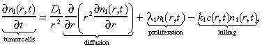
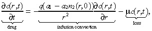
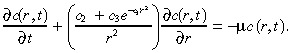
We model the brain using spherical symmetry, where r measures the radial distance from the origin, which represents both the centre of the tumour and the location of the infusion. The mathematical model is a system of partial differential equations that tracks the spatio‐temporal evolution of three entities: the density of tumour cells n ₁(r,t), the density of normal brain cells n ₂(r,t), and the concentration of an infused cytotoxic agent, c(r,t). In the model, the drug is infused at a constant rate for T time units, i.e. for t ∈ [0,T]. Following the Burgess et al. (1997) model, we assume that the tumour cells diffuse freely in the brain and proliferate exponentially. This is in contrast to solid tumours, which are typically modelled as a compact sphere that varies in size over time (Adam & Bellomo 1997). The equation describing the spatio‐temporal dynamics of the tumour cells is:

(1)

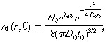
where D ₁ is the diffusion coefficient, λ₁ is the net proliferation rate (mitosis rate minus apoptosis rate), and k ₁ is the rate at which the drug kills the glioma cells. The initial condition for the brain tumour is determined as in Burgess et al. (1997). We set:

(2)

which is the solution to the diffusion (with coefficient D ₀ rather than D ₁, as explained in the first paragraph of Appendix A) plus proliferation equation at time zero if the tumour starts from a point source of N ₀ cells at time –t ₀. While Equation 2 is quite simple, it has been shown that several generalizations, such as incorporating irregular fronto‐temporal growth patterns or the physical boundaries of the domain in which the tumour is growing, do not significantly alter the results of the model (Woodward et al. 1996).

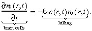
The normal brain cells in our model neither diffuse nor proliferate, but are simply killed by the treatment at rate k ₂:

(3)

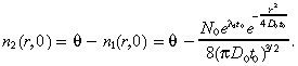
We assume that the total (normal plus tumour) cell concentration in the brain at time 0 equals the constant value θ, so that the initial condition for the normal brain cells is:

(4)

The two primary modes of transport for macromolecules in tissue are diffusion and convection (Swabb et al. 1974). In the case of an infused substance in the brain, convection caused by infusion dominates the effect of diffusion (Morrison et al. 1994). More specifically, infusing a 52‐kDa macromolecule such as IL4(38–37)‐PE38KDEL (Puri et al. 1996; Husain et al. 1998; Rand et al. 2000), which has a diffusion coefficient in brain tissue of 2.54 × 10⁻⁷ cm²/s (using Saltzman & Radomsky 1991 and equation (F) in Swabb et al. (1974)), at a rate of 6 µl/min (see Table 1) generates the Peclet number (i.e. the bulk‐to‐diffusive flow ratio) at a radial distance r cm from the point of infusion. Hence, the Peclet number drops to 10 at a distance of 1.31 cm, and to 5 at a distance of 5.24 cm, implying that little radial diffusion occurs within the practically relevant range. Consequently, we ignore diffusion of the infused agent in this model. The drug concentration at location r at time t is given by:

Table 1.

Parameter values for the model

Parameter	Estimate
Tumour diffusion coefficient after time 0, D 1	0
Tumour growth rate, λ1	1.4 × 10−7 s−1
Drug killing rate of tumour, k 1	67.9 cm3 µg−1 h−1
Initial size of tumour at point source, N 0	1.19 × 106 cells
Time to grow from point source to presentation, t 0	4.26 × 107 s
Tumour diffusion coefficient before time 0, D 0	1.5 × 10−8 cm2 s−1
Drug killing rate of normal cells, k 2	1.27 × 10−3 cm3µg−1 h−1
Cell density, θ	2.04 × 107 cells cm−3
Tumour convection constant, a 1	267.2
Tissue convection constant, a 2	1.3 × 10−5 cm3 cells−1
Drug loss rate, µ	8.35 × 10−4 s−1
Infusion rate, q	6 µL min−1
Time duration of infusion, T	96 h
Concentration of injected fluid, c 0	9 µg cm−3
Clonogenic fraction of tumour cells, f 1	1.19 × 10−7
Toxic fraction of normal cells, f 2	0.01
Radius for calculating toxicity, R̂	5 cm

(5)

where q is the infusion rate, a ₁ and a ₂ are convection constants in the tumour and normal tissue, respectively, and µ is the loss rate divided by the extracellular fraction [see Morrison et al. (1994) for details about modelling the extracellular compartment]. The first‐order loss term in Equation 5 implies that binding is unsaturated, and also captures the loss due to bulk flow across microvasculature walls via a microvascular Peclet analysis [see equations 2 and 2(a) in Morrison et al. (1994) for details]. The infusion convection term in Equation 5 attempts to capture both the spatial heterogeneity of brain cells and tumour cells, and the fact that infused agents follow the tumour trail (i.e. penetrate the tumour more easily than the tissue) (Dillehay 1997). To motivate this term, let us for the moment assume that the drug is travelling through a homogeneous collection of tumour cells. Then n ₂(r,0) = 0 and the convection term in Equation 5 reduces to:

(6)

which is the term derived in Morrison et al. (1994) by calculating the interstitial velocity using Darcy's Law and a conservation of mass equation. Similarly, if we assumed that the agent was travelling through a tumourless brain, we would obtain the convection term:

(7)

which again is of the same form. The general convection term in Equation 5 makes the simplistic but reasonable assumption that the convection constant is a spatially weighted average of the convection constants for tumour and tissue, where the weight at location r depends on the local fraction of tumour cells and normal cells at time 0. Because very little diffusion of tumour cells occurs during the course of treatment (which is typically several days), our use of n ₂(r,0) rather than n ₂(r,t) in the convection term in Equation 5 is justified and greatly simplifies the analysis. Note that the constants a ₁ and a ₂ are expressed in different units (see Table 1) and a ₁ (a ₂, respectively) increases (decreases, respectively) with the ease of convection. The boundary condition for Equation 5 is:

c (0, t ) =  c₀  for  t   ∈   [0, T ], (8)

where c ₀ is the drug concentration in the injection. In Equation 8, we are setting the catheter radius, which is about 0.03 cm (Morrison et al. 1994), to zero.

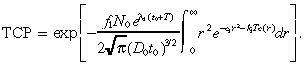
To compute the tumour cure probability (TCP), we employ the commonly used ‘Poisson model’ (Tucker & Taylor 1996), which states that the TCP is e ^−CT, where C_T is the number of clonogenic cells (i.e. cells capable of tumour regeneration) at the end of treatment. If we let f ₁ be the fraction of tumour cells that are clonogenic, then:

(9)

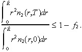
We assume toxic complications are experienced if a fraction f ₂ of the normal cells present at time 0 within a radius R̂ of the origin are killed by time T. That is, toxicity occurs if:

(10)

(9), (10) implicitly assume that the total number of tumour cells (normal cells, respectively) is minimized (maximized, respectively) precisely at the end of treatment. This is a good assumption when the clearance rate µ is high, as it is in our numerical calculations [based on data from IL‐4(38–37)‐PE38KDEL in 1998, 1999 )]. However, for a slow‐clearing agent, it is likely that the tumour burden (total normal cell killing, respectively) will be minimized (maximized, respectively) at some point after treatment, in which case it would be more accurate to incorporate postinfusion diffusion of the agent, as described by Morrison et al. (1994 ).

Our best estimates for the parameter values appear in Table 1. The derivations of these values are discussed in Appendix A.

RESULTS

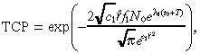
In Appendix B we derive approximate but accurate expressions for n ₁(r,T), n ₂(r,T) and TCP. The approximate TCP is given by:

(11)

which is expressed in terms of the constants:

(12)

(13)

and

(14)

Our computational study uses (26), (30) rather than Equation 11 to compute the TCP because the former expression is slightly more accurate. Because IL‐4(38–37)‐PE38KDEL specificity does not appear to be the dose‐limiting factor for treatment (Rand et al. 2000), our computational study focuses primarily on the TCP rather than on the toxicity of normal tissue in Equation 10.

Base case

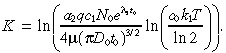
To understand the base case, we plot in Fig. 1b, a and d the steady‐state drug concentration, and the spatial profiles of the tumour cell concentration at the beginning and end of treatment, respectively. The actual characteristic distance (i.e. inflection point) of the drug penetration in Fig. 1b is 2.57 cm, which is intermediate between the characteristic distance of the drug in tumour cells (4 cm) and normal brain cells (1 cm), reflecting the fact that the drug is travelling through a heterogenous mixture of tumour and brain cells.

Figure 1.

The spatial profiles of (a) the initial tumour cell density, (b) the steady‐state drug concentration, (c) the probability of tumour cell survival, and (d) the final tumour cell density.

Figure 1c plots e ^{– k 1 Tc ( r )} , which represents the probability that a tumour cell located at radius r survives treatment. By Equation 28 in Appendix B, the spatial profile of tumour cells at the end of treatment ( Fig. 1d ) is proportional to the product of the spatial profiles of the initial tumour cell density ( Fig. 1a ) and the probability of cell survival during treatment ( Fig. 1c ). Because the spatial concentration of initial tumour cells in Fig. 1a decreases more slowly, according to:

(15)

than the sharp rise in cell survival in Fig. 1c, the spatial profile for the tumour cells at the end of treatment in Fig. 1d is unimodal and the left tails of the curves in Fig. 1c and d are nearly identical in shape. Figure 1 reveals that an increase in TCP can be achieved by shifting the curve in Fig. 1a to the left (via earlier detection) or shifting the curve in Fig. 1c to the right (e.g. via an increase in the infusion rate). The curve in Fig. 1d is proportional to the product of the curves in Fig. 1a and c.

Although our focus is on tumour cure, numerical simulations (not shown here) of our model show that tumour relapse occurs, typically within 1 cm of the tumour margin, if a cure is not achieved. Indeed, our model builds on the models in Tracqui et al. (1995), Woodward et al. (1996) and Burgess et al. (1997), which are calibrated using relapse data after surgery and chemotherapy.

The remainder of this section is devoted to examining the impact of the various parameters on TCP. The model parameters fall into three categories: tumour characteristics, drug design and drug delivery.

Tumour characteristics

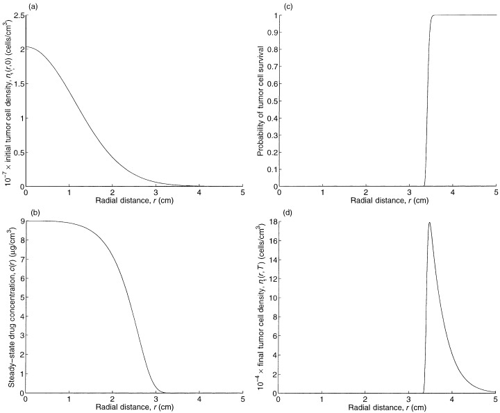
We do not continuously vary each tumour parameter in isolation because these parameters are interrelated in a complex way. Rather, we compute the TCP for the other three tumours considered in Burgess et al. (1997). In addition to a high grade tumour that represents our base case, the numerical study in Burgess et al. (1997) considers a low grade tumour, which has a proliferation rate λ₁ and a diffusion coefficient D ₀ that are reduced by a factor of 10 relative to the high grade tumour; a high proliferation tumour, which has only the diffusion coefficient reduced by a factor of 10; and a high diffusion tumour, which has only the proliferation rate reduced by a factor of 10. For all four tumours in Burgess et al. (1997), the parameter N ₀ has the fixed value given in Table 1, and the value of t ₀ is chosen so that the detectable tumour cell density, 8 × 10⁶ cells per cm³, is achieved at a radius of 1.5 cm, as shown in 1, 2. The resulting TCPs are 0.99 for the high proliferation tumour, 0.0 for the high diffusion tumour, and 0.23 for the low grade tumour. Because very little proliferation or diffusion takes place during the short duration of treatment, these somewhat puzzling results can be explained by viewing the initial tumour cell profiles for these three cases, which are depicted in Fig. 2. The initial spatial profiles of the high grade tumour in Fig. 1a and the low grade tumour in Fig. 2b are very similar, and this similarity carries over to their TCPs. In contrast, the high proliferation tumour in Fig. 2a has a more concentrated spatial profile (e.g. n ₁(r,0) = 0.35 cells per cm³ at r = 3 cm) and the high diffusion tumour has a more dispersed spatial profile. Consequently, the infused agent (see Fig. 1b) has an easy time penetrating the high proliferation tumour but is unable to spread throughout the high diffusion tumour. Hence, assuming that detection occurs when a detectable tumour cell density is achieved at a detectable tumour radius, the TCP depends almost entirely on the diffusion‐to‐proliferation ratio, rather than on the absolute values of these two quantities.

Figure 2.

The spatial profiles for the initial tumour cell density for the three lower grade tumours in Burgess et al. (1997 ): (a) the high proliferation, and (b) the high diffusion and low grade tumours.

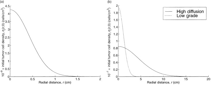
To assess potential improvements in detection technology, we also continuously vary the time of detection t ₀ for our base case tumour. The plot of TCP as a function of t ₀ is given in Fig. 3a. The initial detectable tumour radius r(t ₀), which is defined as the radius that achieves the detectable tumour cell density of 8 × 10⁶ cells per cm³, is given by:

Figure 3.

The impact of time of detection on (a) TCP and (b) the detectable tumour radius.

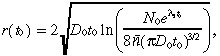(16)

where n̄ = 8 × 10⁶ cells per cm³, and is plotted in Fig. 3b. Although the detectable tumour radius is only growing at a rate of several mm per month in Fig. 3b, Fig 3a suggests that earlier detection of the tumour (relative to the base case of t ₀ = 16.2 months) would significantly improve the TCP.

Drug design

Figure 4a plots TCP versus the drug potency k ₁ c ₀ , which we define as the product of the killing rate and the drug concentration of the injected fluid. Although this curve is increasing, it is quite flat: e.g. a greater than 100‐fold increase in potency is required to raise the TCP from 0.2 to 0.3.

Figure 4.

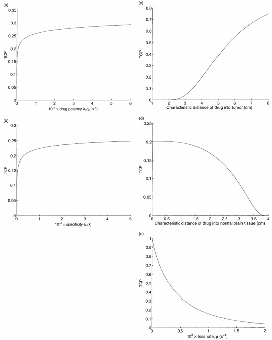
TCP versus drug design parameters: (a) drug potency, (b) drug specificity, (c) drug penetration into tumour, (d) drug penetration into normal brain cells, and (e) loss rate.

Now we incorporate the toxicity of normal brain tissue. We vary the specificity k ₁/k ₂ by multiplying the value of k ₁ in Table 1 and dividing the value of k ₂ in Table 1 by the same factor. For a given value of this factor, we set the infusion duration T so that Equation 10 is satisfied with equality, and compute the corresponding TCP. Using the value of f ₁ in Table 1 yields a TCP of 0.16 for our base case for this computational experiment, rather than the value of 0.2 used for all of the other experiments. This discrepancy in the base case TCPs is consistent with the fact that our estimate of k ₂ is based on data for transferrin‐CRM107 (Laske et al. 1997b), which is a less specific agent than IL4‐PE (see Appendix A for details). The resulting graph of TCP versus specificity is pictured in Fig. 4b. Even though this curve is increasing, a 100‐fold increase in specificity over the base case only leads to a TCP of 0.25, reflecting the fact that drug penetration, which is not affected by drug specificity, is also required to cure the tumour.

Figure 4c and 4d plot TCP versus the convection parameters a ₁ and a ₂ . To ease the interpretation of these parameters, we express them in terms of the corresponding characteristic distances in tumour and brain tissue, respectively (see Appendix A for details). Although a ₁ does not directly appear in (26), (30) for the TCP, it impacts TCP by causing changes in our determination of a ₂ , as described in Appendix A. Increasing the tumour characteristic distance leads to better spatial coverage of the tumour by the drug, and to an increase in TCP in Fig. 4c . The relationship is roughly linear in the neighbourhood of our base case: each additional cm of drug penetration raises the TCP by about 0.2. In contrast, increasing the tissue characteristic distance leads to a reduction in TCP in Fig. 4d , because less drug is delivered to the tumour. The characteristic distances in tumour and brain tissue are determined primarily by the size of the macromolecule, and so in practice both of these distances would be changed simultaneously.

Figure 4e contains a plot of TCP versus the drug loss rate µ. A reduction in the loss rate increases drug penetration, and significantly improves the TCP. Our model slightly underestimates the enhancement in TCP due to a reduction in loss rate, because if the loss rate gets too small then post‐treatment drug diffusion occurs that can increase the spatial drug distribution.

Drug delivery

The drug delivery parameters are the infusion rate q and the infusion duration T. In Fig. 5a, we plot TCP versus q for a fixed infusion volume qT. In Fig. 5b, we fix the infusion rate q and vary the infusion time T. In Fig. 5a, the TCP increases in the infusion rate, and the effect is significant in the practically relevant range (q = 10 µl/min causes catheter tract leaks in Laske et al. (1997)). The TCP initially increases in the infusion duration T in Fig. 5b, but the curve is flat in the vicinity of our base case of T = 96 h, and even begins to decrease at T = 135 h. To explain this behaviour, note that as T increases, more new tumour cells are produced and more cell killing occurs. Because the drug concentration quickly attains its steady‐state profile and because the killing rate and loss rate are high, tumour cell killing exhibits decreasing returns to scale with respect to T. Eventually, tumour growth dominates the trade‐off, leading to a reduction in TCP with increasing T.

Figure 5.

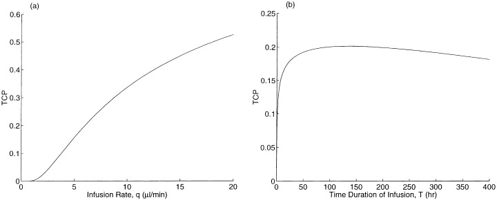
TCP versus drug delivery parameters: (a) infusion rate for a fixed infusion volume, and (b) time duration of infusion.

DISCUSSION

Our mathematical model employs aspects of the brain tumour model described by Burgess et al. (1997) and the model for the delivery of microinfused macromolecules in the brain as described by Morrison et al. (1994), and combines them to capture the spatio‐temporal dynamics of drug transport and killing in a heterogeneous collection of tumour cells and normal brain cells.

Implications of results

Equation 11 provides an explicit equation for the TCP in terms of model parameters describing the tumour characteristics, drug design and drug delivery. The formula itself provides several nonobvious insights. For example, TCP depends on the tissue convection parameter a ₂ , the infusion rate q and the drug clearance rate µ via a ₂ q /µ. Hence, our model predicts that a 50% increase in the convection parameter, a 50% increase in the infusion rate, and a 50% decrease in the mean time‐to‐clearance would each achieve an equivalent increase in TCP. All of the key parameters have a monotonic (i.e. either increasing or decreasing) impact on TCP, with the exception of the duration of infusion T . For a drug with a restricted spatial distribution, when T gets too large the marginal cell killing from an increase in T is more than offset by tumour proliferation during treatment. The nature of the monotonic impact on TCP by the other model parameters is intuitive, with the possible exception of the tissue convection parameter a ₂ . Increasing the ease of convection in tissue without changing the convection in the tumour causes the tumour to retain less of the agent, thereby reducing the TCP.

Figure 1 reveals that the TCP achieved by a highly selective agent in our model is dictated largely by the spatial profile of the pretreatment cell density ( Fig. 1b ) and the steady‐state drug concentration (which impacts the cell survival curve in Fig. 1c ). Hence, high specificity is necessary but not sufficient for curing a highly malignant glioma; a highly concentrated spatial profile of pretreatment tumour cells and/or a deep distribution of infused drug is also required. With regards to the former, our results show that the TCP is affected by the tumour diffusion and proliferation parameters almost solely through their ratio, with relatively invasive tumours being much more difficult to cure than relatively fast‐growing tumours. Moreover, our model predicts that advances in detection technology, even if they only reduce the time of detection by several months, are likely to significantly improve TCP.

The second approach to improving TCP, better drug distribution, can be achieved by a variety of drug design and delivery parameters. We find that the most promising approaches are an increased drug infusion rate, a decreased drug loss rate and a smaller macromolecule. In contrast, infusion duration has a limited impact on TCP, and huge improvements in drug specificity and drug potency are required to significantly enhance TCP. Hence, traditional chemotherapeutic agents – even if distributed with state‐of‐the‐art technology – appear incapable of generating profound improvements in TCP of highly invasive gliomas.

Model limitations

Our approach in this paper is to develop the simplest possible model that both captures the first‐order effects of brain tumour treatments and is amenable to an approximate closed‐form expression for TCP. Consequently, the model is a highly simplified representation of an actual injected tumour. Although the tumour in our model is spherically symmetric, and the brain lacks barriers and boundaries, this tumour model has been validated against clinical data for untreated tumours and for surgical resection (Woodward et al. 1996; Burgess et al. 1997). One restrictive assumption in our model is that no drug resistance occurs. (1), (2) (except without the spatial aspects of drug delivery) have been shown to require two populations of cells – one sensitive and one resistant – to accurately mimic the clinical effect of traditional chemotherapy (Burgess et al. 1997). However, the present model is geared at highly specific agents that target receptors on tumour cells, and drug resistance may not be as much of an issue in this setting. For example, IL‐4 receptor expression appears to be a stable phenomenon: tumour cells remained sensitive to IL‐4 cytotoxins upon repeat administration in vivo (Laske et al. 1997b; Husain et al. 1998), after surgical resection in vitro (Laske et al. 1997b; Husain et al. 1998), and after becoming resistant to certain chemotherapeutic agents (e.g. doxorubicin and mitoxantrone) (De Jong et al. 2000).

Our modelling of drug delivery (see Equation 5) captures the heterogeneity of brain and normal tissue, but is highly simplified. Nonetheless, a special case of Equation 5, which models drug delivery into normal brain tissue, compares reasonably well with laboratory data (Morrison et al. 1994). Two key aspects ignored in Equation 5 are saturated binding and diffusion. Saturated binding might cause the infusion time to impact the spatial distribution, which would increase this parameter's impact on TCP. Diffusion would only play a significant role if the drug was cleared very slowly.

A third aspect ignored in Equation 5 is the heterogeneity of drug delivery between tumour cells and necrotic debris. An infusate can ‘streak’ or ‘channel’ through necrotic portions of a tumour, thus leaving a significant fraction of the tumour without the drug (e.g. Boucher et al. 1997). While drug streaking may occur in the rightmost region of Fig. 5b, subjective evidence suggests that this phenomenon did not occur in the clinical setting of Laske et al. (1997b) and Rand et al. (2000), where necrosis was massive and appeared to be homogeneously distributed. Hence, further quantitative studies are required to understand the clinical prevalence of drug streaking. Drug streaking cannot be captured by our model, and a more complex radially asymmetric model would be required to mimic this behaviour. If drug streaking is found to be clinically significant in future studies, the agent should be delivered at both a high infusion rate (to reach the outer limits of the tumour) and at a low infusion rate (to offset the drug streaking and saturate the tumour bed).

The injection regime is the simplest possible: a constant infusion rate into the centre of the tumour for a finite period of time. Undoubtedly, more complex regimens – both temporally (Bobo et al. 1994; Dillehay et al. 1997) and spatially (Rand et al. 2000) – can improve performance, but these issues are beyond the scope of this paper.

While our Poisson model for TCP is widely used for solid tumours, this assumption is virtually impossible to validate for brain tumours due to the invasive nature of gliomas and the concomitant measurement difficulties.

Also, our modelling of normal tissue complications is quite crude. In fact, dose‐limiting complications can be due not only to lack of specificity, but to brain oedema caused by a high infusion rate or a large infusion volume, or to swelling caused by massive tumour necrosis (Rand et al. 2000). While constraints placed on the infusion rate q and the infusion volume qT are easily assessed by our model, further research and new strategies, possibly requiring repeated dosings and craniotomies (Rand et al. 2000), are required to understand and overcome dose‐limiting complications due to tumour necrosis.

Finally, our baseline value of 0.2 TCP is arbitrary, and is not meant to reflect the actual TCP of IL‐4‐PE, IL‐4(38–37)‐PE38KDEL, transferrin‐CRM107 or any other cytotoxic agent (although this value is not inconsistent with preliminary results for IL‐4(38–37)‐PE38KDEL, where 1 of 9 glioblastoma multiforme patients appear to be tumour‐free 18 months after treatment (Rand et al. 2000)). Hence, our numerical results are indicative of relative, not absolute, efficacy. Nonetheless, for a drug that offers partial cure rates (i.e. TCP not near 0 or 1) for certain grades of gliomas, our results suggest which further improvements might be most beneficial.

In summary, new developments in brain tumour research have produced highly specific agents that provide some hope of improving the poor prognosis of malignant gliomas. Our analysis, which is partially illuminated in Fig. 1 and which culminates in the TCP formula in Equation 11, attempts to provide some insights into the impact on TCP that might be achievable by various advances in tumour detection, drug design and drug delivery.

Appendix a

Parameters in Table 1 .

The values for the tumour parameters λ₁ (which corresponds to a tumour doubling time of about 60 days), D ₀ (derived from the observed wave speed of a brain tumour of 0.1 cm per week), N ₀ and t ₀ are taken from Burgess et al. (1997) and are representative of a high grade glioma. The values for N ₀ and t ₀ are chosen so that the tumour cell density at 1.5 cm from the tumour centre achieves the detection limit of 8 × 10⁶ cells per cm³ after t ₀ time units. Because very little diffusion of tumour cells occurs during the course of therapy (at a speed of 0.1 cm/week, the tumour only travels about 0.6 mm during the course of treatment), we set D ₁ = 0 (hence, the need to differentiate between D ₀ and D ₁ in (1), (2), which allows for a more tractable analysis.

The drug killing rate k ₁ was calculated using data for IL‐4‐PE administered to a U251 glioblastoma cell line; 10 ng cm⁻³ concentration of the agent caused 65% cell death at 2 h and 91% cell death at 4 h. Hence:

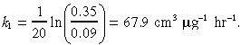(17)

A natural value for θ is the maximum value of the tumour cell concentration, so that there are no normal brain cells at the very centre of the tumour. By Equation 2, this yields:

(18)

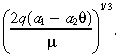
To estimate the tumour convection parameter a ₁, suppose that the drug was infused into a collection of tumour cells, so that n ₂(r,0) = 0 in Equation 5. Then the characteristic distance, which is the distance to the inflection point of the steady‐state solution of the drug concentration, is:

(19)

and the time to approach this characteristic distance is 2/(3µ) (Morrison et al. 1994). Using the value of µ in Table 1, this latter quantity is only 13 min, which is far less than the length of treatment (T = 96 h). Hence, it is reasonable to estimate a ₁ by equating the characteristic distance to the observed distance that IL‐4(38–37)‐PE38KDEL travels in the tumour, which is about 4 cm. Equating 4 cm to:

(20)

yields the value of a ₁ in Table 1. Similarly, we derive a ₂ by equating the observed distance the IL‐4(38–37)‐PE38KDEL travels in white matter (1 cm) to the characteristic distance of a drug that is infused into a tumorless brain:

(21)

Husain et al. (1999 ) state that 30% of IL‐4(38–37)‐PE38KDEL remains at the tumour site after intratumour administration in a subcutaneous tumour model at 2 h after treatment. Hence, we estimate the loss rate to be:

(22)

As in Morrison et al. (1994), we divide this loss rate by the extracellular fraction, which we take to be 0.2, to obtain the value in Table 1.

The volumetric flow rate q, the length of infusion T, and the injected concentration c ₀ in Table 1 are representative of the IL‐4(38–37)‐PE38KDEL regimen. These values correspond to a total dose of 311 µg and a total infused volume of 34.56 cm³.

Data to estimate values of f ₁ and f ₂ are not available. Because our computational study contains a sensitivity analysis with respect to most of the parameters, we did not want the TCP of the base case to be too close to 0 or 1. Hence, we arbitrarily set f ₁ so that the TCP for the data in Table 1 is 0.2. We arbitrarily set f ₂ = 0.01 and R̂ = 5 cm to determine toxicity. Finally, a baseline value for the normal cell killing rate k ₂ is determined by assuming that c ₀ = 1 µg cm⁻³, which is the concentration that causes toxicity of transferrin‐CRM107 in Laske et al. (1997b), satisfies expression Equation 10 with equality.

Appendix b

Mathematical analysis

This appendix contains an approximate analytical derivation of the solution to (1), (2), (3), (4), (5), (8), (9). For ease of presentation, let us define the constants:

(23)

Then substituting Equation 4 into Equation 5 gives:

(24)

For the parameter values in Table 1 and for practical values of r, it follows that c ₂ << c ₃ e ^–c1r2. Hence, we set c ₂ equal to zero in Equation 24; numerical computations (not shown here) confirm that this approximation is highly accurate. Moreover, as explained earlier, the characteristic time for the infusion in the tumour is only about 13 min, which is much less than the length of treatment, and so we replace c(r,t) in (1), (3) by its steady‐state value, which we denote by c(r). With these two approximations in hand, c(r) satisfies the ordinary differential equation:

(25)

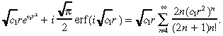
Using separation of variables, we find that the solution to (8), (25) is:

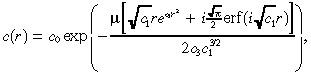(26)

where i =  and erf(x) is the error function

(27)

Substituting Equation 26 into (1), (3), setting D ₁ = 0, and integrating yields:

(28)

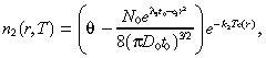(29)

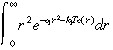
Substituting Equation 28 into Equation 9 gives:

(30)

(26), (30) are used to generate the numerical results in the paper. However, in an attempt to derive a closed‐form expression for the TCP, we now make two further approximations: we approximate c ( r ) in Equation 26 and approximate the integral in Equation 30 . To approximate c ( r ) in Equation 26 , we first note that ( Abramowitz & Stegun 1972 , page 297):

(31)

Making the approximation:

(32)

we approximate the right side of Equation 31 by r(e ^c1r2 − 1), which has been confirmed (data not shown) to be highly accurate. Substituting this expression into Equation 26 yields our approximate value for c(r):

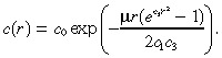(33)

To simplify the integral in Equation 30, we use Fig. 1c to justify approximating e ^–k1Tc(r) by a step function that jumps from 0 to 1 at r̂, where e ^–k1Tc(r) = 0.5. That is, we approximate: 

(34)

by:

(35)

Using the approximation c(r) in Equation 33, we can express the equation for r̂ as:

(36)

where K is defined in Equation 14. Because we expect c ₁r̂² > 1, we use the Taylor series approximation:

(37)

to express

(38)

in Equation 36 by

(39)

Similarly, we expect ln r̂ < c ₁r̂², and so we use the Taylor series approximation:

(40)

After these two Taylor series approximations, Equation 36 becomes:

(41)

We use an iterative method to approximate the solution r̂ to Equation 41. If we ignore the

(42)

term in Equation 41 then the solution is

(43)

Now we subsititute

(44)

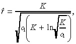
r into the right side of Equation 41 and solve for r , which yields the expression in Equation 13 of the text.

Performing the integration

(45)

and substituting into Equation 30 yields

(46)

Although we imposed a slew of approximations to derive Equation 46, each of these approximations was highly accurate and the resulting TCP in Equation 46 for the base case is 0.197, which is very close to the value of 0.2 computed via (26), (30). Further computations confirm that Equation 46 is a reliable estimate of TCP over a wide range of parameter values. Finally, we note that erf(x) ≈ 1 for x > 2. Hence, we make the approximation:

(47)

in Equation 46 to obtain Equation 11 of the text. This last approximation is slightly less accurate, leading to a TCP of 0.229 in the base case. Nonetheless, numerical computations reveal that Equation 11 only slightly overestimates the TCP for a wide variety of cases, and hence captures all of the qualitative features of our model. An analagous sequence of approximations that led from (28), (29), (30), (31), (32), (33), (34), (35), (36), (37), (38), (39), (40), (41), (42), (43), (44), (45), (46) can be used to simplify n ₂(r,T) in Equation 29, but we omit the details.

REFERENCES

- Abramowitz M, Stegun IE (1972) Handbook of Mathematical Functions. Applied Mathematics Series 55. Washington, DC: National Bureau of Standards. [Google Scholar]
- Adam JA, Bellomo N (1997) A Survey of Models for Tumor‐Immune System Dynamics. Boston, MA: Birkhäuser. [Google Scholar]
- Basser PJ (1992) Interstitial pressure, volume, and flow during infusion into brain tissue. Microvascular Res. 44, 143. [DOI] [PubMed] [Google Scholar]
- Bobo RH, Laske DW, Akbasak A, Morrison PF, Dedrick RL, Oldfield EH (1994) Convection‐enhanced delivery of macromolecules in the brain. Proc. Natl Acad. Sci. USA 91, 2076. [DOI] [PMC free article] [PubMed] [Google Scholar]
- Boucher Y, Salehi H, Witwer B, Harsh IVGR, Jain RK (1997) Interstitial fluid pressure in intracranial tumours in patients and in rodents. Br. J. Cancer 75, 829. [DOI] [PMC free article] [PubMed] [Google Scholar]
- Burgess PK, Kulesa PM, Murray JD, Alvord EC Jr (1997) The interaction of growth rates and diffusion coefficients in a three‐dimensional mathematical model of gliomas. J. Neuropath. Exp. Neurol. 56, 704. [PubMed] [Google Scholar]
- Chen MY, Lonser RR, Morrison PF, Governale LS, Oldfield EH (1999) Variables affecting convection‐enhanced delivery to the striatum: a systematic examination of rate of infusion, cannula size, infusate concentration, and tissue‐cannula sealing time. J. Neurosurg. 90, 315. [DOI] [PubMed] [Google Scholar]
- De Jong MC, Scheffer GL, Slootsra JW, Broxterman HJ, Meloen RH, Husain SR, Joshi BH, Puri RK, Scheper RJ, (2000) Activity of a recombinant interleukin‐4‐pseudomonas exotoxin is reduced in tumor cell lines overexpressing the multidrug resistance protein MRP1, but not cell lines overexpressing P‐glycoprotein, breast cancer resistance protein, MRP2 or MRP3. 91st Annual Meeting Amer. Assoc. Cancer Res. April 1–5, 2000. Abstract #4294. Vol. 41, p. 675 San Francisco, CA: Amer. Assoc. Cancer Res. [Google Scholar]
- Dillehay LE (1997) Decreasing resistance during fast infusion of a subcutaneous tumor. Anticancer Res. 17, 461. [PubMed] [Google Scholar]
- Husain SR, Behari N, Kreitman RJ, Pastan I, Puri RK (1998) Complete regression of established human glioblastoma tumor xenograft by interleukin‐4 toxin therapy. Cancer Res. 58, 3649. [PubMed] [Google Scholar]
- Husain SR, Kreitman RJ, Pastan I, Puri RK (1999) Interleukin‐4 receptor‐directed cytotoxin therapy of AIDS‐associated Kaposi's sarcoma tumors in xenograft model. Nature Med. 5, 817. [DOI] [PubMed] [Google Scholar]
- Laske DW, Morrison PF, Lieberman DM, Corthesy ME, Reynolds JC, Stewart‐Henney PA, Koong S, Cummins A, Paik CH, Oldfield EH (1997a) Chronic interstitial infusion of protein to primate brain: determination of drug distribution and clearance with single‐photon emission computerized tomography imaging. J. Neurosurg 87, 586. [DOI] [PubMed] [Google Scholar]
- Laske DW, Youle RJ, Oldfield EH (1997b) Tumor regression with regional distribution of the targeted TF‐CRM107 in patients with malignant brain tumors. Nature Med. 3, 1362. [DOI] [PubMed] [Google Scholar]
- Lieberman DM, Laske DW, Morrison PF, Bankiewicz KS, Oldfield EH (1995) Convection‐enhanced distribution of large molecules in gray matter during interstitial drug infusion. J. Neurosurg 82, 1021. [DOI] [PubMed] [Google Scholar]
- Morrison PF, Dedrick RL (1986) Transport of cisplatin in rat brain following microinfusion. J. Pharm. Sci. 75, 120. [DOI] [PubMed] [Google Scholar]
- Morrison PF, Laske DW, Bobo H, Oldfield EH, Dedrick RL (1994) High‐flow microinfusion: tissue penetration and pharmacodynamics. Am. J. Physiol. 266, R292. [DOI] [PubMed] [Google Scholar]
- Puri RK, Hoon DS, Leland P, Snoy P, Rand RW, Pastan I, Kreitman RJ (1996) Preclinical development of a recombinant toxin containing circularly permuted interleukin 4 and truncated pseudomonas exotoxin for therapy of malignant astrocytoma. Cancer Res. 56, 5631. [PubMed] [Google Scholar]
- Puri RK, Leland P, Kreitman RJ, Pastan I (1994) Human neurological cancers express interleukin‐4 receptors which are targets for the toxic effects of IL‐4‐Pseudomonas exotoxin chimeric protein. Int. J. Cancer 58, 574. [DOI] [PubMed] [Google Scholar]
- Rand RW, Kreitman RJ, Patronas N, Varricchio F, Pastan I, Puri RK (2000) Intratumoral administration of recombinant circularly permuted interleukin‐4‐pseudomonas exotoxin in patients with high grade glioma. Clin. Cancer Res. (Adv. Brief) 6, 2157. [PubMed] [Google Scholar]
- Saltzman WM, Radomsky ML (1991) Drugs released from polymers: diffusion and elimination in brain tissue. Chem. Engr. Sci. 46, 2429. [Google Scholar]
- Swabb EA, Wei J, Gullino PM (1974) Diffusion and convection in normal and neoplastic tissues. Cancer Res. 34, 2814. [PubMed] [Google Scholar]
- Swanson K (1999) Mathematical modeling of the growth and control of tumors. PhD Dissertation. Seattle, WA: Department of Applied Mathematics, University of Washington.
- Tracqui P, Cruywagen GC, Woodward DE, Bartoo GT, Murray JD, Alvord EC Jr (1995) A mathematical model of glioma growth: the effect of chemotherapy on spatio‐temporal growth. Cell Prolif. 28, 17. [DOI] [PubMed] [Google Scholar]
- Tucker SL, Taylor JMG (1996) Improved models of tumour cure. Int. J. Radiat. Biol. 70, 539. [DOI] [PubMed] [Google Scholar]
- Woodward DE, Cook J, Tracqui P, Cruywagen GC, Murray JD, Alvord EC Jr (1996) A mathematical model of glioma growth: the effect of extent of surgical resection. Cell Prolif. 29, 269. [DOI] [PubMed] [Google Scholar]