Proteogenomic analysis of human colon cancer reveals new therapeutic opportunities

Summary

We performed the first proteogenomic study on a prospectively collected colon cancer cohort. Comparative proteomic and phosphoproteomic analysis of paired tumor and normal adjacent tissues produced a catalogue of colon cancer-associated proteins and phosphosites, including known and putative new biomarkers, drug targets, and cancer/testis antigens. Proteogenomic integration not only prioritized genomically inferred targets, such as copy number drivers and mutation-derived neoantigens, but also yielded novel findings. Phosphoproteomics data associated Rb phosphorylation with increased proliferation and decreased apoptosis in colon cancer, which explains why this classical tumor suppressor is amplified in colon tumors and suggests a rationale for targeting Rb phosphorylation in colon cancer. Proteomics identified an association between decreased CD8 T cell infiltration and increased glycolysis in microsatellite instability-high (MSI-H) tumors, suggesting glycolysis as a potential target to overcome the resistance of MSI-H tumors to immune checkpoint blockade. Proteogenomics presents new avenues for biological discoveries and therapeutic development.

Graphical Abstract

One sentence

A systematic proteogenomic analysis of colon cancer reveals vulnerabilities of potential clinical value inaccessible from genomic assessment alone.

Introduction

Colorectal cancer (CRC) is the third most common cancer worldwide and the fourth leading cause of cancer-related deaths (Arnold et al., 2017). Recent studies of the genomic, transcriptomic, and proteomic landscapes of human CRC have identified many genomic alterations and have revealed extensive molecular heterogeneity of the disease (Cancer Genome Atlas Network., 2012; Guinney et al., 2015; Zhang et al., 2014). However, the rapidly accumulating omics data have yet to bring novel biomarkers and drug targets to the clinic.

Global proteomic differences between tumor and normal tissues, which are critical for cancer biomarker discovery, have not been systematically characterized in large tumor cohorts. Signaling proteins and pathways are often attractive therapeutic targets for cancer treatment, yet global phosphoproteomic analyses on human CRC are lacking. Recent advances in cancer immunotherapy underscore the critical need for biomarkers to predict response to immune checkpoint inhibition and to select neoantigens for personalized vaccine development (Sharma et al., 2017). Proteogenomics can provide fresh approaches to these needs. Here we describe a proteogenomic study from the Clinical Proteomic Tumor Analysis Consortium (CPTAC) on a prospectively collected colon cancer cohort to systematically identify new therapeutic opportunities.

Results

Proteogenomic profiling

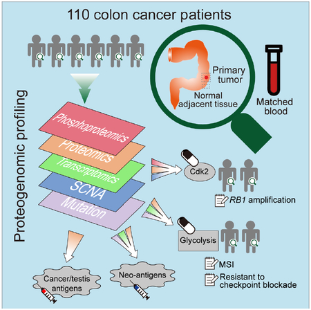
We prospectively collected tumor specimens, matched normal adjacent tissues (NATs), and blood samples from 110 colon cancer patients. We performed whole-exome sequencing (WXS), copy number array, RNA-Seq, miRNA-Seq, and label-free shotgun proteomic analyses on the tumor samples, similar to our previous study (Zhang et al., 2014). To characterize the proteomes in cancer and normal states, we further performed isobaric tandem mass tag (TMT) labeling-based global and phosphoproteomic analysis on both tumors and NATs (Figure 1A). Table S1 summarizes the clinical and pathological characteristics of the tumors.

Figure 1. Schematic overview of the study.

(A) Samples and omics platforms for data generation. (B) Therapeutic hypothesis generation through proteogenomic integration. The colors in B represent data generated from different omics platforms as indicated by the same colors in A.

Although this study includes only colon tumors, rather than both colon and rectal tumors in The Cancer Genome Atlas (TCGA) cohort (Zhang et al., 2014), the average mRNA profiles were highly correlated between the two cohorts (Pearson’s r = 0.92) as were the average label-free protein profiles (Pearson’s r = 0.96), and these correlations were higher than those between different cancer types or between colon tumors and cell lines (Figure S1A-G). Principal component analysis clearly separated the tumors and NATs based on the TMT global or phosphoproteomics data and no batch effect was observed between the TMT plexes (Figure S1H-I). Correlation of proteomics data between the label-free and TMT platforms was higher than for either with RNA-Seq data (Figure S1J-L). Label-free proteomics data from colon tumors outperformed RNA-Seq data for gene function prediction, and TMT data further outperformed both (Figure S1M-O). These results affirm the consistency of the two proteomic platforms and the added value of proteomics for assessing gene functions. Based on the comprehensive molecular profiling datasets, we performed integrative proteogenomic data analyses, focusing on using global and phosphoproteomics data to improve the interpretation of genomics data and to reveal new therapeutic opportunities (Figure 1B).

Somatic mutations and their proteomic consequences

WXS analysis of 106 tumor specimens and matched blood samples identified 64,010 somatic single nucleotide variants (SNVs) and 7,691 somatic insertions/deletions (INDELs) (Figure S2A-B). A focused analysis of microsatellites further identified 6,186 somatic microsatellite INDELs (MS INDELs, Figure S2C, Table S2). In total, we identified 56,592 unique somatic protein altering events (Table S3).

The number of MS INDELs showed a clear bimodal distribution, which allowed us to separate the samples into a microsatellite instability-high (MSI-H) group (n=24) and a microsatellite stable (MSS) group (n=82, Figure S2D). For the 85 samples with PCR-based MSI testing results, WXS-based assignment agreed completely with PCR assignment (Table S2). MSI-H tumors showed a distinct mutational spectrum with an increased proportion of A>G/T>C transitions and decreased G>C/C>G transversions compared to MSS tumors (Figure S2E). The MSI-H group was enriched with mutations in the mismatch repair pathway and in the POLE and BRAF genes (Figure S2F).

To identify significantly mutated genes, we grouped the MSI-H and the one hypermutated MSS sample with a POLE mutation into a hypermutated group; the remaining samples formed a non-hypermutated group (Figure S2D). In the non-hypermutated group, we identified eight significantly mutated genes (Figure 2A), which all were reported in the TCGA study (Cancer Genome Atlas Network., 2012). In the hypermutated group, we identified nine significantly mutated genes (Figure 2B), six of which were not reported in the TCGA study. Four genes newly identified in this study, namely CASP5, RNF43, LTN1, and BMPR2, were mutated in more than 50% of the hypermutated samples.

Figure 2. Somatic mutations and their proteomic consequences.

(A-B) Significantly mutated genes in non-hypermutated (A) and hypermutated (B) samples. Mutation frequency is shown at the top for each gene. Genes not reported in the TCGA study are shown in bold font. (C-F) Somatic mutations vs protein/phosphosite abundance change for APC (C), TGFBR2 (D), TP53 (E), and SOX9 (F). For each gene, the top panel lollipop plot visualizes all protein altering somatic mutations detected in this cohort. The size of a lollipop represents the number of samples with corresponding mutation, and the color represents a specific type of mutation as indicated in the figure legend. The location of the post-translational modification (PTM) of interest is indicated by a triangle. The bottom panel co-visualizes the mutation and protein or phosphosite abundance data for individual samples. For mutation data, a colored box denotes the existence of a specific type of mutation as indicated in the figure legend. Grey boxes indicate data are not available. If a given sample has more than one type of mutation, only one type is shown in the following order of priority: stop-gain, frameshift-INDEL, non-frameshift INDEL, and non-synonymous SNV. In the waterfall plot, each bar represents the protein or phosphosite abundance change between tumor and matched normal adjacent tissue for a patient. Red and green bars represent over- and under-expression in tumor, respectively. White space in the waterfall plots indicates missing values.

The TMT data on matched tumors and NATs allowed us to investigate the proteomic consequences of somatic mutations. Some protein changes could be predicted from the mutations, such as the stop-gain and frameshift mutations in APC, which result in nonsense-mediated mRNA decay or truncated proteins. As expected, tumors with these mutations had reduced abundance of phosphosite APC-T2451, which is located downstream of the mutations (Figure 2C). Similarly, tumor samples bearing frameshift mutations in TGFBR2 showed reduced abundance of phosphosite TGFBR2-S553 (Figure 2D).

Some protein changes were difficult to predict based on the mutations. For example, phosphorylation of TP53-S315 was increased in tumors over matched NATs (p = 0.001, paired t-test). Three tumors with more than 10-fold increase of TP53-S315 phosphorylation all had an R273 mutation (Figure 2E). We reviewed TP53-S315 phosphorylation data from the CPTAC breast (Mertins et al., 2016) and ovarian cancer (Zhang et al., 2016) studies and found TP53-S315 phosphorylation in tumors with R273 mutations was 3.4- to 83-fold above the medians of those cohorts, strengthening the association between these hotspot mutations and increased TP53-S315 phosphorylation.

The high mobility group (HMG) transcription factor SOX9 was recurrently mutated in this cohort, including six stop-gain mutations, eight frameshift mutations, and five nonsynonymous SNVs. According to the “20/20 rule” that classifies genes with more than 20% truncating mutations as tumor suppressor genes (Vogelstein et al., 2013), SOX9 should be classified as a tumor suppressor. However, SOX9 protein was significantly overexpressed in tumor samples compared to matched NATs (p = 1.02×10⁻¹⁰, paired t-test, Figure 2F), which argues against a tumor suppressor assignment. Even in tumors with the truncating mutations, despite the small number of samples, we still observed statistically significant overexpression of SOX9 (p = 0.04, paired t-test, Figure 2F). Interestingly, most of the truncating mutations occurred downstream of the HMG-box domain and upstream of the evolutionally conserved ubiquitin-target site K398 (Figure 2F), which is responsible for 26S proteasome dependent degradation of SOX9 (Akiyama et al., 2005). Thus, removal of the K398 ubiquitination site through the truncating mutations may stabilize SOX9 protein and increase protein abundance. Consistent with these data, functional assays support an oncogenic rather than tumor suppressor role of SOX9 in primary CRC cells (Matheu et al., 2012).

Taken together, our somatic mutation analyses identified new significantly mutated genes among MSI-H tumors, and the proteomics data revealed unexpected functional complexity that could not have been predicted from mutation data alone.

Proteomics data prioritize somatic copy number alterations

We performed somatic copy number alteration (SCNA) analyses with WXS data and Illumina SNP array data, but the SNP array data showed low dynamic range. Hence, we only report SCNAs identified from WXS analysis. We identified very similar arm level SCNAs to the TCGA cohort, including amplifications of 1q, 7p and q, 8p and q, 13q, and 20p and q, and deletions of 1p, 14q, 15q, 17p and q, 18p and q, and 22q (Figure 3A). Focal level SCNAs (Figure 3B) did not completely agree with those reported in the TCGA study, which may reflect cohort and/or platform differences. Nonetheless, most focal SCNAs previously reported were found in our cohort. Cytobands in chromosome 20 (20p12.1, 20q13.12, 20q13.13) and chromosome 18 (18q21.2) contained the most frequently amplified and deleted focal regions, respectively (Figure 3B).

Figure 3. Somatic copy number alteration (SCNA) analysis.

(A) Arm-level SCNA events. Red denotes amplification and blue denotes deletion. (B) Focal-level SCNA events. Focal peaks with significant copy number gains (red) and losses (blue) (GISTIC2 Q-values < 0.25) are shown. The top ten amplified and deleted cytobands are labeled, with the proportions of amplified or deleted samples shown in the parentheses. Representative genes encoded from these focal peaks are highlighted in approximate positions across the genome. (C) Effects of copy number alternations on mRNA and protein abundance. The upper heatmap panel shows the abundance of significant copy number correlation with mRNA (left) and protein (right). Significant positive and negative correlations (adj. p < 0.01, Spearman’s correlation coefficient) are indicated by red and blue, respectively. Genes are ordered by chromosome locations on both x- and y-axes. The bottom panel shows the frequency of significant correlations. Grey bars represent copy number correlation to mRNA (left) and protein (right), and black bars represent copy number correlation to both mRNA and protein. (D) Strategy for prioritizing genes in focal alteration peaks. (E) Most enriched KEGG pathways and Gene Ontology (GO) biological processes (BP) for genomic drivers inferred in this study. (F) Six deleted genes involved in endocytosis. Violin plots compare protein expression in tumor and normal adjacent tissue for each gene.

Next, we examined the correlations of SCNA with mRNA and protein abundance. While cis-effects of SCNAs on mRNA abundance were similar to our previous study (Zhang et al., 2014), cis-effects on protein abundance were stronger (Figure 3C), reflecting the greater quantitative precision of the TMT platform compared to the previous label-free analysis. We also confirmed previously reported trans-acting SCNA hot spots on chromosomes 20q, 18, 16, 13 and 7 and identified a new hot spot on chromosome 14 (Figure 3C).

Previously, we showed that correlated copy number, mRNA, and protein levels can prioritize copy number drivers in focal alteration regions. Here we found that only 59% of such prioritized amplification or deletion drivers showed expected protein-level effects in tumor versus NAT comparisons (Figure 3D). Thus, data from NATs can substantially refine candidate driver lists (Table S4). The final prioritized list included the previously reported 20q amplification drivers HNF4A and TOMM34. We also identified the well-known tumor suppressor SMAD4 in the 18q focal deletion region.

To better understand the genomic drivers inferred in this study, including the 17 significantly mutated genes and the 90 prioritized SCNA genes, we performed enrichment analysis. Not surprisingly, significantly enriched terms included colorectal cancer, cell proliferation, cell death, and Hippo signaling pathway (Figure 3E). Enrichment for endosome organization and endocytosis, including six genes located in different focal deletion regions across the genome (Figure 3F), indicated that multiple deletion events converge to repress the endocytosis pathway, which may allow tumors to gain self-sufficiency in growth signals (Mosesson et al., 2008).

Rb phosphorylation as a driver and therapeutic target in colon cancer

One of the recurrently amplified genes in this cohort was the retinoblastoma (RB1) gene (Figure 4A). Consistently, the RB1 protein (Rb) was overexpressed in tumors compared to NATs (p = 2.10×10⁻¹⁵, paired t-test, Figure 4B). RB1 was the first tumor suppressor gene identified, and its amplification and overexpression in colon cancer contradict its frequent mutation and deletion in other cancers (Figure S3).

Figure 4. Rb phosphorylation as a driver and therapeutic target in colon cancer.

(A-C) RB1 Copy number alteration (CNA) (A), protein log2 fold change (FC) from normal (B), and phosphorylation log2 fold change from normal (C). Samples are ordered by increasing average phosphorylation abundance. (D-E) Correlations of Rb protein abundance change (D) and average Rb phosphorylation change (E) with estimated E2F1 activity change. (F-H) Correlation of average Rb phosphorylation change with estimated CDK2 activity change (F), H3.1 phosphorylation change (G), and protein level changes of apoptotic proteins (H). (I) A model depicting the multi-level regulation of RB1 in colon cancer, highlighting Rb phosphorylation as a driver and therapeutic target in colon cancer.

As a tumor-suppressor, Rb prevents cell proliferation by inhibiting E2F transcription factors, but this inhibition is abolished by Rb phosphorylation (Rubin, 2013). Phosphoproteomics quantified six Rb phosphorylation sites in at least 50% of all samples, including four sites (i.e., T373, S807, S811, and T826) that regulate E2F binding (Knudsen and Wang, 1997; Rubin, 2013). The average abundance of the four sites was higher in colon tumors than in NATs (p < 2.2×10⁻¹⁶, paired t-test) (Figure 4C). Moreover, the average tumor vs NAT change for phospho-Rb was 1.84-fold, which was significantly higher (p=0.01, Wilcoxon signed-rank test) than the 1.58-fold average change for total Rb measured from global proteomics. Thus, tumor samples had not only higher total Rb, but also a higher proportion of phospho-Rb within the total Rb pool.

Predicted E2F1 activity changes between tumors and NATs (STAR Methods) were positively correlated with both total Rb change (Pearson’s r = 0.40, p = 5.1×10⁻⁵, Figure 4D) and phospho-Rb change (Pearson’s r = 0.30, p = 3.5×10⁻³, Figure 4E). Because un-phosphorylated Rb inhibits E2F1 activity, the significant positive correlation between total Rb and E2F1 activity suggests that the increase of total Rb in tumors is attributable to phospho-Rb, rather than un-phosphorylated Rb. The positive correlation between E2F1 activity and phospho-Rb may reflect a positive feedback loop (Sherr and McCormick, 2002), in which E2F1 transcriptionally upregulates cyclin E, which activates CDK2, thereby phosphorylating Rb and relieving E2F1 inhibition of cell proliferation. Indeed, phospho-Rb change showed the highest correlation with the predicted activity change of CDK2 (r = 0.47, p = 1.8×10⁻⁶, Figure 4F) compared to all other kinases (STAR Methods). Further, phospho-Rb change was significantly correlated with the phosphorylation change of histone H3.1, a marker for cell proliferation (Pearson’s r = 0.49, p = 2.6×10⁻⁴, Figure 4G). Therefore, our data showed that increased Rb phosphorylation, instead of RB1 mutation or deletion, drives colon cancer proliferation. However, it remains puzzling why RB1 is recurrently amplified in colon tumors, because post-translational down-regulation of the inhibitory activity of this over-expressed protein seems mechanistically inefficient. Further analysis showed that Rb phosphorylation change in colon tumors was negatively correlated with the apoptosis hallmark gene set (STAR Methods, Pearson’s r = −0.28, p = 5.3×10⁻³, Figure 4H), which primarily comprises pro-apoptotic genes (Liberzon et al., 2015). Thus, phospho-Rb appears to have an antiapoptotic role.

Together, proteogenomic data integration suggests that Rb phosphorylation regulates both proliferation and apoptosis to drive colon cancer development (Figure 4I). This insight reveals a previously unexploited opportunity to target Rb phosphorylation in colon cancer through CDK2 inhibition, which is not possible for cancers driven by RB1 mutation or deletion.

Colon cancer-associated proteomic events and potential clinical utilities

TMT global proteomic analysis of the 96 tumor and NAT pairs identified a total of 8,067 proteins. Among the 6,422 proteins that were quantified in at least 50% of the samples (i.e., quantifiable proteins), 2,217 (35%) were significantly increased and 2,527 (39%) were significantly decreased in tumors compared to paired NATs (adj. p < 0.01, Wilcoxon signed-rank test, Figure 5A). Of these, 31 increased and 417 decreased proteins had a more than 2-fold abundance change. The 417 proteins elevated in NATs were significantly enriched in muscle-related functions (Figure 5B), as expected from normal colon histology, which includes defined muscular structures that are typically absent in tumors. We focused our analysis on the 31 proteins elevated by more than 2-fold in tumors, which we defined as colon cancer-associated proteins (Table S5).

Figure 5. Colon cancer-associated proteomic events.

(A) Volcano plot indicating proteins over-expressed in tumors or normal adjacent tissues (NATs, light red and blue colors indicate adj. p < 0.01 (sig) whereas red and blue further require more than 2-fold change); other genes are colored in grey. (B) Gene Ontology Biological Processes enriched for the 417 proteins down-regulated in tumors. Venn diagram depicts the overlap between muscle system process related genes and the 417 proteins. (C) Log2-fold change between tumor and matched NATs is shown for the 31 cancer-associated proteins (mean in red). (D) Tumor-cell specific immunohistochemistry (IHC) staining scores defined by the Human Protein Atlas (HPA). (E) Overlap with plasma proteins, secreted proteins, transmembrane proteins, and enzymes annotated by HPA, as well as known clinical utilities. (F) Volcano plot indicating phosphosites over-expressed in tumors or NATs. Colors are the same as in A. (G) Correlation between tumor-normal protein and phosphorylation site abundance differences (Pearson’s r = 0.81, p < 2.2×10⁻¹⁶). The purple dashed line indicates the diagonal line. Red points indicate the phosphorylation sites with greater than 2-fold increase. The black arrows highlight 5 of these phosphorylation sites with lower protein abundance in tumors than in NATs. (H) Overlap of proteins containing cancer-associated phosphorylation sites (Phosphoproteome), cancer-associated proteins (Proteome), and cancer genes in the Cancer Gene Census (CGC). (I) Cancer-associated kinases identified by increased phosphorylation of a known kinase activating site in tumor compared to NAT (phosphorylation) or by phosphosite set enrichment analysis based on known kinase-target site relationships (inferred). Grey boxes indicate data are not available. Black boxes indicate the existence of an FDA-approved drug or a drug undergoing clinical trials targeting that kinase. (J) The number of proteomics-supported neoantigens identified for each sample, with MSI-H and MSS annotation shown at the top. (K) Three cancer/testis (CT) antigens over-expressed by at least 2-fold in tumors compared to NATs in more than 5% of all samples, with the percentage indicated in brackets. Sample order is the same as in J. Grey boxes indicate data are not available.

Figure 5C depicts the distributions of pair-wise tumor-NAT differences for the 31 cancer-associated proteins. Most showed highly homogeneous differential expression across the 96 tumor-NAT pairs. Eight proteins were increased in tumor in more than 95% of the pairs, including DDX21 (100%), S100A11 (100%), RSL1D1 (99%), S100P (97%), RPL36A (97%), PLOD2 (96%), SERPINH1 (95%), and GPRC5A (95%). Among the 30 proteins with immunohistochemistry (IHC) staining data in The Human Protein Atlas (HPA), around half showed medium to strong tumor-specific staining in CRC samples (Figure 5D, Figure S4).

We associated the 31 proteins with the human secretome, membrane proteome, and enzymes because these sub-proteomes are enriched with clinically approved biomarkers and drug targets. Nineteen have been found in plasma, 18 are secreted, nine are trans-membrane, and eight are enzymes (Figure 5E). Fifteen of these proteins have known clinical utilities as diagnostic markers, outcome markers, or therapeutic targets (Table S5), including CEACAM5, which is the most widely used CRC marker in clinical practice (Duffy, 2001). Other proteins may merit further investigation.

We also assessed the differences in phosphorylation site abundance between 96 tumor and NAT pairs. Among the 7,295 phosphorylation sites quantified in at least 50% of the paired samples, 2,119 (29%) were significantly increased and 3,053 (42%) were significantly decreased in tumors compared to paired NATs (adj. p < 0.01, Wilcoxon signed-rank test). Of these, 63 were increased and 793 were decreased with a greater than 2-fold abundance change (Figure 5F). We defined the 63 phosphosites mapping to 50 proteins as cancer-associated phosphosites (Table S5), of which all but one had greater changes in phosphosite abundance than in corresponding protein abundance (Figure 5G, red dots). Despite the overall concordance between phosphosite abundance changes and corresponding protein abundance changes (Pearson’s r = 0.81, p < 2.2×10⁻¹⁶), some cancer-associated phosphosites mapped to proteins that were decreased in tumor samples (Figure 5G, highlighted by black arrows). Only four of the 50 proteins with a cancer-associated phosphosite also met our criteria as cancer-associated proteins. Moreover, only seven proteins in our combined protein set were documented in the Cancer Gene Census, a comprehensive catalogue of genes containing mutations implicated in cancer (Figure 5H). Proteomics and phosphoproteomics data thus are complementary and both reveal additional colon cancer genes that were missed in genomic studies.

Kinases are among the most attractive therapeutic targets for cancer treatment. We predicted cancer-associated kinase activity based on 1) significantly increased phosphorylation of a known kinase activating site in tumor compared to NAT, and on 2) enrichment analysis of the known target sites for each kinase. We identified four kinases by each method, with one kinase, CDK7, identified by both (Figure 5I). Among these kinases, CDK4 is targeted by FDA-approved drugs, and the other CDKs (CDK1, CDK2 and CDK7), MELK, and PFKFB3 are targeted by drugs in clinical trials (Table S5). The last kinase, PI4KB, may merit further investigation as a novel candidate therapeutic target.

Tumor antigens

To facilitate the development of personalized vaccines for cancer immunotherapy, we further analyzed our data to identify candidate tumor antigens, including neoantigens derived from somatic mutations and non-mutated cancer/testis (CT) antigens. To identity candidate neoantigens, We searched the label-free and TMT global proteomics, and TMT phosphoproteomics data against customized protein databases incorporating all coding variations identified from matched exome sequencing and RNA-Seq data and found 173 proteomics-supported somatic mutations. All peptides of 9-11 amino acids in length that contained one of these somatic mutations were evaluated for human leukocyte antigen (HLA)-I binding affinity. The 88 mutant peptides with high predicted binding affinity to HLA molecules were considered as putative neoantigens (Table S6). In total, one or more putative neoantigens were identified for 38% of the tumors (Figure 5J).

The TMT global proteomics data identified a total of 16 CT-antigens, and three were increased by at least 2-fold in tumors compared to paired NATs in more than 5% of all tumor-NAT pairs, including IGF2BP3 (51%), SPAG1 (14%), and ATAD2 (8%) (Figure 5K). According to data in HPA, IGF2BP3 protein expression in normal human tissues is restricted to reproductive organs and fetal brain (Figure S5A). While normal colon tissue stains negatively for IGF2BP3, colon cancer stains positively (Figure S5B). Notably, peptides derived from IGF2BP3 significantly induce a tumor-specific cytotoxic T lymphocyte response in vitro (Suda et al., 2007) and in vivo in human esophageal tumors in a phase I clinical trial (Kono et al., 2009).

In contrast to neoantigens that were enriched in MSI-H tumors and were patient-specific, CT antigens were independent of MSI status and were shared among many patients. Together, we found proteomics-supported neoantigens or CT antigens for 78% of the tumors in this cohort, demonstrating the potential of proteogenomics in identifying tumor antigens for cancer vaccine development.

A unified view of colon cancer molecular subtypes

Applying the consensus molecular subtypes (CMS) classifier (Guinney et al., 2015) to 106 tumors with RNA-Seq data, we assigned 85 (80%) of these tumors to the four transcriptomic subtypes (CMS 1-4, Figure S6A). Applying the CRC proteomic subtype classifier (Zhang et al., 2014) to 100 tumors with label-free proteomics data, we assigned 88 (88%) of these tumors to the five proteomic subtypes (ProS A-E, Figure S6B), and this protein expression pattern was largely preserved in the TMT proteomics data (Figure S6C). These results provided independent validation of the previously published molecular classification systems.

To test for underlying consistency among the mRNA, protein, and MSI-based classifications, we constructed a network, in which nodes represent the subtypes from individual classification systems, and weighted edges represent statistically significant association between two subtypes and the level of significance (Figure 6A). All these associations were confirmed in the TCGA CRC cohort. The connected subtypes in the association network fell naturally into three groups, as indicated by the dashed circles in Figure 6A. The grouping aligned well with previous transcriptomic and proteomic studies that independently associated CMS1 and ProS-B with MSI-H and hypermutation, CMS2 and ProS-E with chromosome instability (CIN), and CMS4 and ProS-C with epithelial-mesenchymal transition (EMT) (Guinney et al., 2015; Zhang et al., 2014). Accordingly, we named the three unified multi-omics subtypes (UMS) as “MSI”, “CIN”, and “Mesenchymal”, respectively. Using a network centrality based weighted voting algorithm, we assigned 87 out of the 110 tumor samples to the three UMS subtypes (Figure 6B). The UMS classification eliminated the CMS3 subtype and assigned CMS3 tumors to other UMS subtypes. This was explained by the vague molecular boundary of the CMS3 subtype (Figure S6D-F). In addition, three MSI-H tumors with relatively fewer MS INDELs were assigned to the Mesenchymal subtype.

Figure 6. A unified, multi-omics view of colon cancer subtypes.

(A) The network representing the association between subtypes defined by genomic (black), transcriptomic (white), and proteomic (grey) classification systems. Edge width denotes the significance of the connections computed by the Fisher’s exact test. The dashed circles indicate the three unified multi-omics subtypes (UMSs). (B) UMS assignment for samples in the cohort. The genomic, transcriptomic, and proteomic subtypes are also shown for comparison. (C) Copy number alteration data grouped by the three UMSs. (D) Stroma and immune infiltration profiles grouped by the three UMSs. The cytotoxic immune cell cluster is highlighted by blue in the dendrogram.

Next, we performed subtype-based supervised analysis on omics data not used in defining the UMS classification. Tumors in the CIN subtype showed higher chromosome instability compared to those in the other two subtypes (p < 0.01, t-test, Figure 6C, Figure S6G), providing orthogonal confirmation of the UMS classification. Similarly, many of the miRNA and phosphosite markers identified in the supervised analysis (Table S7) have known relationships with the subtype-specific features. Examples include decreased expression of miR-552, miR-592, and miR-181d in the MSI subtype (Liu and Zhang, 2016), decreased expression of the miR-200 family in the Mesenchymal subtype (Korpal et al., 2008), and increased phosphorylation of STAT1 and STAT3 in the MSI and Mesenchymal subtypes, respectively (Pensa et al., 2009). Notably, we found higher copy number gain of RB1 in the CIN subtype compared to the other subtypes (Figure S6H). Moreover, Rb-S811 and S807 were significantly increased in the CIN subtype compared to the other subtypes (1.61- and 1.51-fold, respectively), and the increase was much stronger than that of total Rb (1.13-fold, Table S7). These results complement our interpretation of the role of Rb phosphorylation in colon cancer, and further suggest that CDK2 inhibition may be the most effective in the CIN subtype.

To understand the UMS classification in the context of tumor microenvironment, we performed in silico deconvolution to quantify stromal infiltration level, immune infiltration level, and tumor-infiltrating lymphocyte (TIL) subpopulations based on RNA-Seq data. Total stromal infiltration was significantly higher in the Mesenchymal subtype compared to the other two subtypes (Figure 6D). Although both the MSI and the Mesenchymal subtypes had higher immune infiltration than the CIN subtype, the MSI subtype was specifically enriched with cytotoxic immune cells, such as NK cells and activated CD8 T cells, whereas the Mesenchymal subtype was enriched with suppressor immune cells, such as myeloid-derived suppressor cells (MDSCs), macrophages, and Treg cells (Figure 6D). The UMS classification thus provided a unified view of three major subtypes of colon cancers with distinct genomic, transcriptomic, proteomic, and microenvironment profiles.

Increased glycolysis in the MSI subtype is associated with immune suppression

Despite the enrichment of cytotoxic immune cells in the microenvironment, MSI tumors develop and progress, which has been explained by the selective up-regulation of immune checkpoint proteins in the tumor microenvironment (Llosa et al., 2015). However, only a subset of MSI-H CRCs respond to immune checkpoint inhibitors (Le et al., 2015), suggesting a role for other immune evasion mechanisms.

Comparison of protein and mRNA profiles between the MSI subtype and the other UMS subtypes revealed a broad increase of the glycolytic enzymes in the MSI subtype (Figure 7A). We also found an almost universal decrease in tricarboxylic acid (TCA) cycle enzymes at the protein level, but not at the mRNA level. Thus, our data revealed protein-level adaptations driving a strong Warburg effect in the MSI subtype.

Figure 7. Increased glycolysis in the MSI subtype and its association with CD8 T cell infiltration.

(A) MSI subtype-specific alteration of key enzymes involved in the glycolysis and TCA cycle. The MSI subtype-specific RNA and protein changes are shown side-by-side. P values were calculated based on the Wilcoxon rank sum test. (B) The heatmap showing the protein expression levels of glycolytic enzymes within the MSI subtype. Samples are ordered by increased infiltration of activated CD8 T cells. (C) The negative correlation between glycolytic activity (inferred by the protein expression of enzymes involved in the pathway) and the activated CD8 T cell level for the MSI subtype. (D-G) Strong positive correlations were observed between SRM and TMT measurements for CD8A(D), SLC2A3 (E), and PKM2 (F), but not for PKM1 (G). (H) SRM data showed higher CD8A abundance in MSI/CD8-H tumors (n=5) than MSI/CD8-L tumors (n=5). (I-K) SRM data showed higher protein abundance of SLC2A3 (I) and PKM2 (J) in MSI tumors (n=10) compared to CIN (n=5) and Mesenchymal (n=5) tumors, and in MSI/CD8-L tumors (n=5) compared to MSI/CD8-H tumors (n=5). This pattern was not observed for PKM1 (K). (L) Schematic diagram summarizing the interplay between glycolysis and CD8 T cell activation in MSI tumors, highlighting glycolysis as a potential target to overcome the resistance of MSI-H tumors to immune checkpoint blockade.

Lactate, a key product of Warburg effect, is a potent inhibitor of CD8 T cells (Brand et al., 2016). Indeed, almost all glycolytic enzymes were negatively correlated with CD8 infiltration in MSI tumors (Figure 7B). Using the median protein abundance of all glycolytic enzymes as a measure of glycolytic activity, we found a statistically significant negative correlation between glycolytic activity and CD8 infiltration (Spearman’s ρ = −0.61, p = 0.02, Figure 7C). Interestingly, this relationship was not observed in other colon cancer subtypes or when all colon tumors were analyzed together (Figure S7). The interplay between metabolic reprogramming and immune function may apply specifically to immune evasion and checkpoint inhibition resistance in the MSI subtype.

To validate these findings, we performed targeted analysis of selected proteins in representative tumor samples using selected reaction monitoring (SRM). The SRM measurements were highly correlated with TMT measurements for the CD8 T cell marker CD8A (Figure 7D) and the glucose transporter SLC2A3 (Figure 7E). Pyruvate kinase PKM, the rate-limiting glycolytic enzyme that catalyzes the last step of glycolysis, has two isoforms. The targeted SRM analysis also was able to measure isoform-specific peptides that were not detected in the TMT analysis, thereby clarifying that PKM2 was the major isoform measured in the TMT analysis (Figure 7F-G). It is known that PKM2, rather than PKM1, drives aerobic glycolysis and lactate production in human cancer (Christofk et al., 2008). MSI tumors with relatively higher amounts of estimated activated CD8 cells (MSI/CD8-H) had 2.23-fold higher CD8A abundance than those with lower amounts (MSI/CD8-L, Figure 7H), although the difference was not statistically significant, likely due to the expression of CD8A in both activated and inactivated CD8 cells. In the subtype-based comparisons (Figure 7I-K), the abundance of SLC2A3 and PKM2 was 1.85- and 1.4-fold higher (p = 0.007 and 0.003, respectively, t-test) in the MSI subtype compared to the other two subtypes. Within the MSI subtype, SLC2A3 and PKM2 were 1.19- and 1.7-fold higher in the MSI/CD8-L tumors compared to the MSI/CD8-H tumors. These data were consistent with the global proteomics data. Taken together, our data support the model depicted in Figure 7L and suggest that combined therapy of checkpoint and glycolysis inhibition may provide a potent strategy to treat MSI tumors resistant to checkpoint blockade.

Discussion

We performed an unprecedented molecular characterization of human colon cancer and paired NATs with comprehensive integration of data from multiple proteogenomic platforms. Our study confirmed the value of proteogenomic integration in uncovering novel cancer biology and further demonstrated the utility of proteogenomics in therapeutic hypothesis generation.

We combined the customized proteomics database approach with HLA binding prediction and identified personalized neoantigens for 38% of the patients. mRNA expression has been used to prioritize somatic mutations for personalized neoantigen vaccine development, but proteomics-based filtering prioritizes more effectively because neoepitopes themselves are peptides.

Colon cancer-associated proteins and phosphosites identified from our tumor versus NAT comparisons had very little overlap with known cancer genes in the Cancer Gene Census (Figure 5H), providing a novel information layer to our understanding of colon cancer. Notably, several CT antigens were recurrently over-expressed in tumors. In addition to serving as putative tumor-specific biomarkers, the inherent immunogenicity of CT antigens, as demonstrated by IGF2BP3 in esophageal cancer (Kono et al., 2009; Suda et al., 2007), makes them potentially ideal targets for immunotherapy, especially for MSS colon tumors that are poor candidates for checkpoint inhibition or neoantigen vaccine treatment because of their low neoantigen load.

Our multi-omics-based subtype analysis provided a unified view of colon cancer molecular heterogeneity based on three UMS subtypes, i.e., MSI, CIN, and Mesenchymal. Proteomics data associated decreased CD8 infiltration with increased glycolysis in MSI tumors, which supports the emerging view that increased tumor glycolysis suppresses anti-tumor immunity by impairing T cell function and trafficking to the tumor microenvironment (Tang and Fu, 2018). Therefore, glycolysis inhibition may be considered to overcome the resistance of MSI tumors to immune checkpoint blockade.

In addition to reinforcing or complementing genomics data, proteogenomic integration also may correct inaccurate genomics data-based inferences and lead to unexpected discoveries and therapeutic opportunities. One example is the proteomic identification of SOX9 as an oncogene, whereas it was predicted to be a tumor suppressor based on somatic mutation data. Another example is the phosphoproteomics data-enabled discovery of Rb phosphorylation as an oncogenic driver of colon cancer, suggesting a unique opportunity to target Rb phosphorylation in colon cancer through CDK2 inhibition.

In summary, our integrative proteogenomic characterization revealed new therapeutic opportunities for targeting signaling proteins, metabolic enzymes, and tumor antigens in colon cancer treatment. Although validation of these therapeutic hypotheses is beyond the scope of our current study, these new hypotheses may eventually enable substantial advances in molecularly-guided precision therapy of colon cancer. Further interrogation of this deeply characterized colon cancer cohort by other investigators will likely yield additional insights. The primary and processed datasets are available in publicly accessible data repositories and portals (Figure 1A, STAR Methods), and we anticipate broad usage of these datasets for new biological discoveries and therapeutic hypothesis generation.

STAR METHODS

DATA AND SOFTWARE AVAILABILITY

Raw genomics data from this study are available at the Sequence Read Archive (SRA), BioProject ID: PRJNA514017 (ftp://ftp-trace.ncbi.nlm.nih.gov/sra/review/SRP178677_20190114_143443_27e795eb0f314edf0479737480ab0f2a ). Raw and low-level processed proteomics data from this study are available at the CPTAC Data Portal (https://cptac-data-portal.georgetown.edu/cptac/s/S045 ). All final data matrices are available at the LinkedOmics (Vasaikar et al., 2018) (http://linkedomics.org/cptac-colon/ ), which also provides computational tools for further exploration of this dataset.

CONTACT FOR REAGENT AND RESOURCE SHARING

Further information and requests for resources and reagents should be directed to and will be fulfilled by the Lead Contact Bing Zhang (bing.zhang@bcm.edu).

EXPERIMENTAL MODEL AND SUBJECT DETAILS

Specimens and Clinical Data

Tumor, adjacent normal, and blood samples were collected by several tissue source sites in strict accordance to the CPTAC-2 colon procurement protocol (https://brd.nci.nih.gov/brd/sop/download-pdf/321) with an informed consent from the patients. The cohort had an inclusion criterion of newly diagnosed, untreated patients undergoing primary surgery for colon adenocarcinoma. Because untreated rectal tumors are difficult to obtain, we only included colon cancers, which represent approximately 70% of all CRCs. Patients with prior history of other malignancies within 12 months, any systemic chemotherapy, endocrine or biological therapy as well as prior radiation therapy to the abdomen or pelvis for any cancer type were excluded from the study. Required clinical information regarding patient history and status of surgery along with relevant diagnostic information were collected using case reports forms. One year follow up information with updated history after completion of the initial treatment regimen were also collected through follow up forms. Deidentified pathology reports and representative diagnostic slide images were utilized to review and qualify cases for this study. The peripheral venous blood from the same patient were collected prior to administration of anesthesia. Segments from qualified tumor specimens were greater than 300mg in mass with at least 60% tumor cell nuclei and less than 20% necrosis. To ensure tissue suitability for phosphoprotein analysis, the tissue and the adjacent normal specimens were collected in less than 30 minutes total ischemic time and embedded in optimal cutting temperature (OCT) compound for processing at a common CPTAC-2 specimen core resource center. Pathologically qualified cases underwent further molecular qualification for extraction and co-isolation of nucleic acids. Tissue segments that were pathology and molecular qualified were shipped to the proteomic characterization centers. DNA and RNA from the same tumor segment and DNA from germline blood were further aliquoted and quantified per protocol. DNA quality was confirmed using gel electrophoresis and Nano drop methods. RNA quality was confirmed using Nano drop and Agilent bioanalyzer. Sufficient yield, a good gel score and passing value of 7 or greater RIN qualified the DNA and RNA, respectively, for sequencing. The analytes were then shipped to the sequencing center. The corresponding clinical data were formatted and distributed through the CPTAC data coordinating center (https://cptac-data-portal.georgetown.edu/cptac/s/S037). Table S1 summarizes the clinical and pathological characteristics of the tumors and the specific numbers of samples analyzed by each omics platform. Among the 110 patients in the cohort, there were 65 females (60%) and 45 males (40%), with an average age of 65 (range 40 to 93 years). We did not perform analyses on the two sexes separately because the sample size is too small after sex stratification. Moreover, we were interested in results common to both sexes, and the sex distribution is reasonably balanced.

METHODS DETAILS

PCR-based MSI Analysis

The MSI Analysis System (version 1.2, Promega), a fluorescent PCR-based assay, was used to detect microsatellite instability (MSI) in the colon tumors. The analysis compares allelic profiles of microsatellite markers generated by amplification of DNA from matching tumor and normal samples, and alleles that are present in the tumor sample but not in corresponding normal samples indicate MSI. The system uses seven markers including five mononucleotide repeat markers (BAT-25, BAT-26, NR-21, NR-24, and MONO-27) and two pentanucleotide repeat markers (Penta C and Penta D). The output data were analyzed with GeneMapper® software (Applied Biosystems) to determine MSI status of the colon tumor samples.

Genotyping Array Analysis

Genomic DNA samples were prepared according to Illumina’s Infinium LCG Quad Assay manual protocol. Processed samples were loaded on the HumanOmni5-Quad BeadChips and run on the HiScan platform. SNP and CNP genotyping were performed with the Genome Studio Genotyping Module (Version 2.0, Illumina).

Whole Exome Sequencing (WXS)

Genomic DNA samples were used to prepare indexed libraries using the Nextera Rapid Capture Exome kit from Illumina. Library preparation was performed using a semi-automated 96-well plate method, with washing and clean-up/concentration steps performed on the Beckman Coulter Biomek NXP platform and with ZR-96 DNA Clean & Concentrator^™-5 plates, respectively. Libraries were quantified using the Agilent 2100 Bioanalyzer. Pooled libraries were run on HiSeq4000 (2×150 paired end runs) to achieve a minimum of 150x on target coverage per each sample library. The raw Illumina sequence data were demultiplexed and converted to fastq files, adapter and low-quality sequences were trimmed. WXS data were used for somatic mutation detection, microsatellite instability prediction, and somatic copy number alteration (SCNA) analysis as described below.

Somatic Mutation Detection

We followed the Genome Analysis Toolkit (GATK, version 3.8.0) best practice guideline for somatic short variant discovery (https://software.broadinstitute.org/gatk/best-practices/workflow?id=11146). Briefly, we aligned paired-end WXS reads to the human reference genome (hg19) with BWA-mem (version 0.7.15-r1140). The bam files were further processed by adding read groups, marking duplicates, and re-ordering with Picard tools (version 2.9.0). Consequently, base quality score recalibration and INDEL realignment were performed using GATK modules IndelRealigner and BaseRecalibrator. The cross-individual contamination was then estimated by the GATK module ContEst. Single nucleotide variants (SNVs) and INDELs (insertions/deletions) were called from tumor and matched-normal pairs using MuTect2 from GATK. We filtered out variants from short tandem repeat regions, which were downloaded from the UCSC table browser. The sequence variants were then annotated using customProDB and Oncotator. Significance of candidate mutations was evaluated in non-hypermutated and hypermutated tumors separately using MutSigCV (version 1) in GenePattern, and genes with a false discovery rate (q value) below 0.05 were considered significantly mutated above the background mutation rate.

Germline Short Variant Discovery from WXS

We followed the GATK best practice guideline for germline short variant discovery from WXS data (https://software.broadinstitute.org/gatk/best-practices/workflow?id=11145). We started from the processed bam files generated in the previous section. HaplotypeCaller was used to generate an intermediate file, GVCF, for each sample. Next, we consolidated all GVCFs from 106 samples into to one GVCF file using the GATK module CombineGVCF. The merged GVCF file was passed to GenotypeGVCFs, a joint genotyping tool for SNP and INDEL calling. We further filtered the variants by variant quality score recalibration, in which machine learning was used to identify annotation profiles of variants likely to be real.

Microsatellite Instability Prediction

MSMuTect (version 1.0) (Maruvka et al., 2017) was applied to the processed bam files for somatic microsatellite INDEL (MS INDEL) calling. MSMuTect uses the Kolmogorov–Smirnov (KS) test to identify microsatellite sites with different alleles between tumor and normal samples. Using tumors with PCR test results, we found that the Fisher’s exact test provided higher sensitivity and specificity compared to the KS test. Therefore, we applied Fisher’s exact test to the histograms generated by MSMuTect and then used the Fisher’s exact test p-value as the filtering criterion, with a p-value cutoff of 0.001. We named this modified method MSMuTect-fisher. Significant MS INDELs with multiple alleles in normal and only one allele in tumor were removed from further analysis. Using 40 MS INDELs as a cutoff, we separated the samples into an MSI-high (MSI-H) group and a microsatellite stable (MSS) group. MSMutSigCV (Maruvka et al., 2017) was used to detect significantly mutated genes based on identified MS INDELs (p < 0.05).

Annotation of Protein Altering Somatic Mutations

All somatic mutations identified by MuTect2 and MSMuTect, including SNVs, INDELs, and MS INDELs, were annotated using ANNOVAR (Wang et al., 2010). The variants obtained by ANNOVAR were filtered for protein altering events including non-synonymous SNVs, frameshift INDELs, non-frameshift INDELs, and stop gains. Supplementary Table S3 includes all isoforms altered by the somatic mutation events. For the analysis of proteomic consequence, the longest isoform was selected for each somatic mutation event.

Somatic Copy Number Alteration (SCNA) Analysis

SCNA analysis used WXS-derived BAM files that were processed in the somatic mutation detection pipeline. These BAM files were further processed by the R Package CopywriteR (version 1.18.0) (Kuilman et al., 2015), which uses off-target WXS reads to infer copy number values. 105 tumor and matched-normal pairs had sufficient (> 5 million) off-target reads for SCNA detection as recommended by the software (Kuilman et al., 2015). The circular binary segmentation (CBS) algorithm (Olshen et al., 2004) which is also implemented in the CopywriteR package was used for the copy number segmentation, with the default parameters. From the segmentation result, we used a weighted-sum approach to summarize the chromosome instability for each sample. Specifically, the absolute log2 ratios of all segments (indicating the copy number aberration of these segments) within a chromosome were weighted by the segment length and summed up to derive the instability score for the chromosome. The genome-wide chromosome instability index was derived by summing up the instability score of all 22 autosomes.

Next, we used GISTIC2 (version 2.0.23) (Mermel et al., 2011) to retrieve gene-level copy number values and call significant copy number alterations in the cohort. We set up a threshold of 0.4 (-ta and -td parameters of GISTIC2) in picking the amplified or deleted regions based on the distribution of germline copy number variants. Moreover, genome regions containing significant numbers of germline copy number variants were excluded from the GISTIC2 population level statistics (the -cnv parameter of GISTIC2). GISTIC2 generated arm level and focal level SCNAs for the cohort with G-Score and FDR Q value indicating the significance and strength of the identified SCNAs.

In order to prioritize SCNA drivers, we selected all the genes located in the focal region with GISTIC2 Q value less than 0.25. Also, we included genes located in the “wide peaks” identified by GISTIC2. For these genes, spearman correlation was calculated between copy number values and their RNA or protein levels across the cohort. We used FDR less than 0.05 and absolute correlation coefficient larger than 0.3 as the cutoff to select candidate genes. As an additional filtering criterion, we further required candidate amplification and deletion drivers to show significant upregulation and downregulation, respectively, in tumor versus matched adjacent normal comparisons (FDR < 0.05, paired t-test).

mRNA Sequencing

Indexed cDNA sequencing libraries were prepared from the RNA samples using the TruSeq Stranded RNA Sample Preparation Kit and bar-coded with individual tags. Library preparation was performed similarly to the WXS. Quality control was performed at every step, and the libraries were quantified using the Agilent 2100 Bioanalyzer. Indexed libraries were prepared as equimolar pools and run on HiSeq4000 (2×150 paired end runs) to generate a minimum of 30 million paired-end reads per sample library. The raw Illumina sequence data were demultiplexed and converted to. fastq files, and adapter and low-quality sequences were trimmed.

RNA Quantification

mRNA sequencing reads were mapped to the human genome hg19 by STAR (version 2.5.3a) using the 1-pass model. Hg19 sequence and RefSeq annotation were downloaded from the UCSC table browser (03/29/2017). RSEM (version 1.2.31) was used to quantify genes and transcripts expression levels. Gene read counts were calculated using HTseq (version 0.7.2). The RSEM outputs the mRNA RSEM and FPKM (Fragments Per Kilobase of transcript per Million mapped reads) results in table format. The mRNA RSEM data were filtered for genes with median FPKM > 1 for use in downstream analyses.

Short Variant Discovery from RNA-Seq

We followed the GATK Best Practice Variant Detection protocol on RNASeq (http://gatkforums.broadinstitute.org/dsde/discussion/3892/the-gatk-best-practices-for-variant-calling-on-rnaseq-in-full-detail). We used the STAR 2-pass method to align RNA-Seq reads to the human reference genome (hg19). Specifically, splice junctions detected in the 1-pass alignment run were used to guide the 2-pass alignment. After alignment, the SAM file was processed through the usual Picard processing steps including adding read group, sorting, marking duplicates, and indexing. Next, we applied the GATK pipeline including the modules ‘SplitNCigarReads’, ‘HaplotypeCaller’ and ‘VariantFiltration’. The minimum phred-scaled confidence threshold for calling variants was set to 20. The ‘VariantFiltration’ module excluded SNVs with: a quality by depth score (QD) < 2.0, a Fisher strand score (FS) > 30.0, or clusters of at least 3 SNPs that were within a window of 35 bases between them. These filters ensured: (1) high confidence variant calls based on unfiltered depth of non-reference samples (QD); (2) low strand bias for detection of variants (FS)—as strand bias is indicative of false positive calls; and (3) filtering of many false variant calls introduced by RNA-Seq read mapping errors.

miRNA Sequencing

Indexed small RNA sequencing libraries were prepared from the RNA samples using the TruSeq Small Total RNA Sample Prep Kit, and bar-coded with individual tags. Library preparation was performed similarly to the WXS sequencing. Quality control was performed at every step, and the libraries were quantified using the Agilent 2100 Bioanalyzer. Indexed libraries were prepared as equimolar pools and loaded on the NextSeq500 (1×75 single read) run to generate at least 5,000,000 single reads per sample library. The raw Illumina sequence data were demultiplexed and converted to fastq files.

miRNA-Seq Data Analysis

For fastq files from miRNA sequencing, adapters were trimmed using Cutadpt (version 1.13) with a maximum allowed error rate of 0.1. Trimmed reads shorter than 17 or longer than 26 nucleotides in length were excluded from further analysis. Reads were then mapped to the human genome hg19 using Bowtie (version 1.1.1). Mapped reads were then annotated using ncPRO-seq (version 1.6.1) based on the ncPRO-seq hg19 annotation. Mature miRNA annotation was extended 2 bp in both upstream and downstream regions to accommodate inaccurate processing of precursor miRNAs. ncPRO-seq outputs miRNA count and RPM (reads per million mappable reads) results in table format.

Label-free Proteomics Analysis

Label-free shotgun proteomic analyses of the colon tumor samples were done according to the methods described previously (Zhang et al., 2014), with two changes. First, 6 concatenated basic reverse phase LC fractions were prepared from tryptic digests using the same instrumentation described previously. Second, LC-MS/MS analyses were done with a ThermoFisher QExactive MS instrument. LC-MS/MS shotgun proteomics of the concatenated fraction samples were carried out on a Q Exactive mass spectrometer (ThermoFisher Scientific) equipped with an Easy nLC-1000 (ThermoFisher Scientific) and a Nanoflex source (ThermoFisher Scientific). A 2 μL injection volume of peptides were separated on a PicoFrit (New Objective, Woburn, MA) column (75 μm ID × 110 mm, 10 μm ID tip) packed with ReproSil-Pur C18-AQ resin (3 μm particle size and 120 Å pore size). Peptides were eluted at a flow rate of 300 nL/min, and the mobile phase solvents consisted of water containing 0.1% formic acid (solvent A) and acetonitrile containing 0.1% formic acid (solvent B).

A 100-minute gradient was performed, consisting of the following: 0–5 min, increase to 5% B; 5-90 min, 5–35% B; 90-93 min, 90% B; 93-100 min, 90% B and held at 90% B for 7 min before returning to the initial conditions of 2% B. Mass spectra were acquired over the scan range of m/z 300-1800 at a resolution of 70,000 (AGC target 3 ×10⁶ and 64 ms max injection time). Data-dependent scans of the top 20 most abundant ions were selected for fragmentation with HCD using an isolation width of 2 m/z, 27% normalized collision energy and a resolution of 17,500 (AGC target 2 ×10⁵ and 100 ms max injection time). Dynamic exclusion was set to 60 sec.

Label-free Proteomics Data Analysis

The raw MS data were converted to MGF and mzML files using ProteoWizard (version 3.0.10462). The MS/MS data were searched by three search engines (MyriMatch version 2.2.10165, X!Tandem version Alanine 2017.02.01, and MS-GF+ version 2017.01.13) through IPeak (Wen et al., 2015; Wen et al., 2014) against the RefSeq protein database (03/29/2017, 45929 sequences + 245 contaminant sequences) with decoy sequences. The following parameters were set for database searching: Carbamidomethyl (C) was specified as a fixed modification. Oxidation (M) and Deamidated (NQ) were specified as variable modifications. The precursor mass tolerance for protein identification on MS was 10 ppm, and the product ion tolerance for MS/MS was 0.05 Da. Full cleavage by trypsin was used, with up to two missed cleavages permitted. The results from the three search engines were then integrated by IPeak, which is a tool that combines multiple search engine results. To optimize the number of proteins identified we applied a very stringent filter at 0.1% PSM FDR. Then the protein inference was performed and 1% FDR was controlled using the "picked" protein FDR approach (Savitski et al., 2015). To rescue high quality PSMs that were excluded by the stringent PSM FDR threshold, we relaxed the PSM FDR threshold to 1% for the confidently identified proteins.

Spectral count data were filtered by removing proteins with zero counts in all samples and quantile-normalized using the R package preprocessCore (version 1.42.0, https://github.com/bmbolstad/preprocessCore). We further filtered low abundant proteins with average raw count < 1.4 as we did previously (Zhang et al., 2014). The normalized and filtered counts were then log2 transformed for downstream analysis.

Protein Extraction and Tryptic Digestion for TMT Analysis

For TMT analysis, the tumor and normal colon tissue samples were obtained as OCT-embedded tissue curls through the CPTAC Biospecimen Core Resource. Approximately 100 mg of each of the samples were first subjected to OCT removal procedure by sequential rinsing in 70% ethanol, nanopure water, and 100% ethanol. The tissue samples were then homogenized separately in 600 μL of lysis buffer (8 M urea, 100 mM NH₄HCO₃, pH 7.8, 75 mM NaCl, 1 mM EDTA, 10 mM NaF, Sigma phosphatase inhibitor cocktail 2, Sigma phosphatase inhibitor cocktail 3, and 20 μM PUGNAc). Lysates were precleared by centrifugation at 16,500 g for 5 min at 4 °C and protein concentrations were determi ned by BCA assay (Pierce). Proteins were reduced with 5 mM dithiothreitol for 1 h at 37°C, and subsequently alkylated with 10 mM iodoacetamide for 45 min at 25 °C in the dark. Samp les were diluted 1:2 with 100 mM NH₄HCO₃, 1 mM CaCl₂ and digested with sequencing grade modified trypsin (Promega) at 1:50 enzyme-to-substrate ratio. After 3 h of digestion at 37°C, samples were diluted 1:4 with the same buffers and another aliquot of the same amount of trypsin was added to the samples and further incubated at 25°C overnight (~16 h). The digested samples were then acidified with 100% formic acid to 1% formic acid in the final sample solution. Tryptic peptides were desalted on reversed phase C18 SPE columns (Waters tC18 SepPak, 200mg) and dried using Speed-Vac.

TMT-10 Labeling of Peptides

Desalted peptides from each sample were labeled with 10-plex Tandem Mass Tag (TMT) reagents according to the manufacturer’s instructions (ThermoScientific). Peptides (300 μg) from each of the samples were dissolved in 300 μL of 50 mM HEPES, pH 8.5, and mixed with 3 units of TMT reagent that was dissolved freshly in 123 μL of anhydrous acetonitrile. Channel 131 was used for labeling the internal reference sample (pooled from all tumor and normal samples with equal contribution) throughout the sample analysis. After 1 h incubation at RT, 24 pL of 5% hydroxylamine was added and incubated for 15 min at RT to quench the reaction. Peptides labeled by different TMT reagents were then mixed, dried using Speed-Vac, reconstituted with 3% acetonitrile, 0.1% formic acid and were desalted on C18 SPE columns (Waters tC18 SepPak, 200mg).

Peptide Fractionation by Basic Reversed-phase Liquid Chromatography (bRPLC)

Approximately 2.5 mg of 10-plex TMT labeled sample was separated on a Waters reversed phase XBridge C18 column (250 mm × 4.6 mm column containing 5-μm particles, and a 4.6 mm × 20 mm guard column) using an Agilent 1200 HPLC System. After the sample loading, the C18 column was washed for 35 min with solvent A (5 mM ammonium formate, pH 10.0), before applying a 100-min LC gradient with solvent B (5 mM ammonium formate, pH 10, 90% acetonitrile). The LC gradient started with a linear increase of solvent A to 10% B in 6 min, then linearly increased to 30% B in 86 min, 10 min to 43% B, 5 min to 55% B and another 8 min back to 100% B. The flow rate was 0.5 mL/min. A total of 96 fractions were collected into a 96 well plate throughout the LC gradient. These fractions were concatenated into 12 fractions by combining 8 fractions that are 12 fractions apart (i.e., combining fractions #1, #13, #25, #37, #49, #61, #73, and #85; #2, #14, #26, #38, #50, #62, #74, and #86; and so on). For proteome analysis, 5% of each concatenated fraction was dried down and re-suspended in 2% acetonitrile, 0.1% formic acid to a peptide concentration of 0.1 μg/μL for LC-MS/MS analysis. The rest of the concatenated fractions (95%) were further concatenated into 6 fractions by combining two concatenated fractions (i.e., combining concatenated fractions #1 and #7; #2 and #8; and so on), dried down, and subjected to immobilized metal affinity chromatography (IMAC) for phosphopeptide enrichment.

Phosphopeptide Enrichment Using IMAC

Fe³⁺-NTA-agarose beads were freshly prepared using the Ni-NTA Superflow agarose beads (QIAGEN) for phosphopeptide enrichment. For each of the 6 fractions, peptides were reconstituted to 0.5 μg/μL in IMAC binding/wash buffer (80% acetonitrile, 0.1% formic acid) and incubated with 20 μL of the 50% Fe³⁺-conditioned NiNTA bead suspension for 30 min at RT. After incubation, the beads were washed 2 times each with 100 μL of wash buffer on the stage tip packed with 2 discs of Empore C18 material. Phosphopeptides were eluted from the beads on C18 using 60 μL of Elution Buffer (500 mM K₂HPO₄, pH 7.0). 50% acetonitrile, 0.1% formic acid was used for elution of phosphopeptides from the C18 stage tips. Samples were dried using Speed-Vac, and later reconstituted with 10 μL of 3% acetonitrile, 0.1% formic acid for LC-MS/MS analysis.

LC-MS/MS for TMT Global Proteome Analysis

The global proteome fractions were separated using a nanoAquity UPLC system (Waters Corporation) by reversed-phase HPLC. The analytical column was manufactured in-house using ReproSil-Pur 120 C18-AQ 1.9 μm stationary phase (Dr. Maisch GmbH) and slurry packed into a 30-cm length of 360 μm o.d. × 75 μm i.d. fused silica containing a 3-mm sol-gel frit. The trapping column was manufactured in-house using Jupiter 300 C18 5-μm stationary phase (Phenomenex) and slurry packed into a 4-cm length of 360 μm o.d. × 150 μm i.d. fused silica with the final column being sol-gel fritted on both ends. The analytical column was heated to 50°C using an AgileSLEEVE column heater (Analytical Sales and Services, Inc.). The analytical column was equilibrated to 95 % Mobile Phase A (MP A, 0.1% formic acid in water) and 5% Mobile Phase B (MP B, 0.1% formic acid in acetonitrile) and maintained at a constant column flow of 200 nL/min. The sample injected (5-μL) was trapped using 100% MP A for 10 min at flow rate of 3 μL/min before being placed in-line with the analytical column and subjected to the gradient profile (min: %MP B): 0:5, 1:8, 44:15, 85:30, 94:55, 102:70, 105:95, 108:95, 115:5, 150:5.

MS analysis was performed using a Q-Exactive Plus mass spectrometer (Thermo Scientific, San Jose, CA). Electrospray voltage (2.2 kV) was applied at a carbon composite union (Valco Instruments Co. Inc.) between the analytical column and electrospray emitter (chemically etched 360-μm o.d. × 20-μm i.d.). The ion transfer tube was set at 250 °C. Following a 15-min delay from the end of sample trapping, Orbitrap precursor spectra (AGC 1×10⁶) were collected from 300-1800 m/z for 120 minutes at a resolution of 70K along with the top 12 data dependent Orbitrap HCD MS/MS spectra at a resolution of 35K (AGC 1×10⁵) and max ion time of 100 msec. Masses selected for MS/MS were isolated at a width of 0.7 m/z and fragmented using a normalized collision energy of 32%. Peptide match was set to ‘Preferred’, exclude isotopes was set to ‘on’, and charge state screening was enabled to reject unassigned 1+, 7+, 8+, and >8+ ions with a dynamic exclusion time of 20 sec to discriminate against previously analyzed ions.

LC-MS/MS for TMT Phosphoproteome Analysis

The phosphoproteome fractions were separated using a nanoAquity UPLC system (Waters Corporation) by reversed-phase HPLC. The analytical column was manufactured in-house using ReproSil-Pur 120 C18-AQ 1.9 μm stationary phase (Dr. Maisch GmbH) and slurry packed into a 35-cm length of 360 μm o.d. × 50 μm i.d. fused silica picofrit capillary tubing (New Objective, Inc.). The trapping column was manufactured in-house using Jupiter 300 C18 5-μm stationary phase (Phenomenex) and slurry packed into a 4-cm length of 360 μm o.d. × 150 μm i.d. fused silica with the final column being sol-gel fritted on both ends. The analytical column was heated to 50°C using an AgileSLEEVE column heater. The ana lytical column was equilibrated to 98 % MP A and 2% MP B and maintained at a constant column flow of 120 nL/min. The sample injected (5 μL) was trapped using 100% MP A for 5 min at a flow rate of 3 μL/min before being placed in-line with the analytical column and subjected to the gradient profile (min:%MP B): 0:2, 8:4, 50:15, 85:35, 94:60, 95:95, 105:95, 115:2, 170:2.

MS analysis was performed using an Orbitrap Fusion Lumos mass spectrometer (Thermo Scientific). Electrospray voltage (1.8 kV) was applied at a Valco carbon composite union coupling a 360 μm o.d. × 20 μm i.d. fused silica extension from the LC gradient pump to the analytical column and the ion transfer tube was set at 250°C. Following a 40-min delay from the end of sample trapping, Orbitrap precursor spectra (AGC 4×10⁵) were collected from 350-1800 m/z for 120 min at a resolution of 60K along with data dependent Orbitrap HCD MS/MS spectra (centroided) at a resolution of 50K (AGC 1×10⁵) and max ion time of 105 msec for a total duty cycle of 2 seconds. Masses selected for MS/MS were isolated (quadrupole) at a width of 0.7 m/z and fragmented using a collision energy of 30%. Peptide mode was selected for monoisotopic precursor scan and charge state screening was enabled to reject unassigned 1+, 7+, 8+, and >8+ ions with a dynamic exclusion time of 45 sec to discriminate against previously analyzed ions between +/− 10 ppm.

Quantification of TMT Global Proteomics Data

LC-MS/MS analysis of the TMT10-labeled, bRPLC fractionated samples generated a total of 264 global proteomics data files. The Thermo RAW files were processed with DTARefinery (Petyuk et al., 2010) (v1.2) to characterize and correct for any instrument calibration errors, and then with MS-GF+ (Kim et al., 2008; Kim and Pevzner, 2014) (v9881) to match against the RefSeq human protein database (03/29/2017, 45929 sequences), combined with 261 contaminants (e.g., trypsin, keratin). The partially tryptic search used a +/−10 ppm parent ion tolerance, allowed for isotopic error in precursor ion selection, and searched a decoy database composed of the forward and reversed protein sequences. MS-GF+ considered static carbamidomethylation (+57.0215 Da) on Cys residues and TMT modification (+229.1629 Da) on the peptide N-terminus and Lys residues, and dynamic oxidation (+15.9949 Da) on Met residues for searching the global proteome data.

Peptide identification stringency was set at a maximum false discovery rate (FDR) of 1% at peptide level using PepQValue < 0.005 and parent ion mass deviation < 7 ppm criteria. A minimum of 6 unique peptides per 1000 amino acids of protein length was required for achieving 1% at the protein level within the full data set. Inference of parsimonious protein set resulted in the identification of a total of 8,067 common protein groups among the 197 samples.

The intensities of all ten TMT reporter ions were extracted using MASIC software (Monroe et al., 2008). Next, PSMs passing the confidence thresholds described above were linked to the extracted reporter ion intensities by scan number. The reporter ion intensities from different scans and different bRPLC fractions corresponding to the same gene were grouped. Relative protein abundance was calculated as the ratio of sample abundance to reference abundance using the summed reporter ion intensities from peptides that could be uniquely mapped to a gene. The pooled reference sample was labeled with TMT 131 reagent, allowing comparison of relative protein abundances across different TMT-10 plexes. The relative abundances were log2 transformed and zero-centered for each gene to obtain final, relative abundance values.

Small differences in laboratory conditions and sample handling can result in systematic, sample-specific bias in the quantification of protein levels. In order to mitigate these effects, we computed the median, log2 relative protein abundance for each sample and re-centered to achieve a common median of 0.

Quantification of Phosphopeptides

Phosphopeptide identification for the 132 phosphoproteomics data files were performed as described above (e.g., peptide level FDR <1%), with an additional dynamic phosphorylation (+79.9663 Da) on Ser, Thr or Tyr residues. The phosphoproteome data were further processed by the Ascore algorithm (Beausoleil et al., 2006) for phosphorylation site localization, and the top-scoring sequences were reported. For phosphoproteomics data, the TMT-10 quantitative data were not summarized by protein, but left at phosphopeptide level. All the peptides (phosphopeptides and global peptides) were labeled with TMT-10 reagent simultaneously. Separation into phospho- and non-phosphopeptides using IMAC was performed after the labeling. Thus, all the biases upstream of labeling are assumed to be identical between global and phosphoproteomics datasets. Therefore, to account for sample-specific biases in the phosphoproteome analysis, we applied the correction factors derived from mean-centering the global proteomics data.

Gene-wise Correlation Between Different Platforms

We calculated gene-wise correlations for each pair of the three platforms, including RNA-Seq, label-free proteomics, and TMT proteomics. For each pair of the platforms, the analysis included the top 10% most variably expressed genes in each platform and quantifiable in both platforms. Spearman’s correlation between the two platforms was calculated for each gene across all the samples.

mRNA and Protein Correlation Across Datasets

We calculated average gene-wise RNA expression and performed the Pearson’s correlation coefficient analysis between the prospective colon tumor samples (N=106) and TCGA CRC samples (N=90) (Zhang et al., 2014), TCGA breast tumor samples (N=1102, downloaded from TCGAbiolinks FPKM-UQ (Colaprico et al., 2016), TCGA ovarian tumor samples (N=374, downloaded from TCGAbiolinks FPKM-UQ), and colorectal cell lines (N=44) (Wang et al., 2017b), respectively. Similarly, we calculated average gene-wise protein expression (label-free) and performed the Pearson’s correlation coefficient analysis between the prospective colon tumor samples (N=100) and TCGA colorectal samples (N=95) (Zhang et al., 2014), colorectal cell lines (N=44) (Wang et al., 2017b), and NCI-60 colorectal cell lines (N=60, quantile-normalized) (Gholami et al., 2013), respectively.

Co-expression-based Gene Function Prediction

To compare the ability of different gene expression profiling datasets to predict gene function, we constructed k-nearest neighbor co-expression networks as previously described (Wang et al., 2017a) using RNA-Seq, label-free proteomics, and TMT proteomics data, respectively. Network-based gene function prediction was performed using the random walk-based network propagation algorithm (Wang et al., 2017a). Prediction performance was evaluated using 5-fold cross validation for each KEGG pathway and quantified based on the area under the receiver operating characteristic curve (AUROC).

Tumor vs Normal Differential Proteomic Analysis

TMT-based global proteomics data were used to perform differential proteome analysis between tumor and matched normal samples. Gene-level data were further filtered for non-missing values in at least 50% of samples. A paired Wilcoxon signed-rank test was performed on overlapping samples to determine differential abundance of proteins between tumor and normal. Proteins with fold change > 2 and Benjamini-Hochberg adjusted p-value < 0.01 were considered to be cancer-associated proteins. GO enrichment analysis was performed using WebGestalt (Wang et al., 2017c). For each cancer-associated protein, we checked immunohistochemistry images in colorectal tumors from the Human Protein Atlas (HPA, https://www.proteinatlas.org/), in which tumor-specific staining is reported in four levels, i.e. high, medium, low, and not detected. The weighted average score (IHC staining) was calculated for each protein by assigning weight to high, medium, low, and not detected respectively.

Tumor vs Normal Differential Phosphoproteomic Analysis

Identified phosphopeptides were mapped to UniProt sequences (version July 2017), and named according to the canonical UniProt sequence. If the peptide matched multiple canonical UniProt sequences, the best ID was chosen based on presence of the protein in the proteomics data. If no canonical IDs had proteomics data, or if more than one protein was present in the quantified proteomics data, an ID was chosen at random. For peptides not matching a canonical protein sequence, a matching protein isoform ID was chosen. Peptides were filtered to those with an Ascore ≥19 in at least one scan and a Q value < 0.01. Phosphorylation site levels were determined by the median level for all peptides matching that site. Quantified sites and proteins were defined as those containing non-missing values in at least 50% of the matched samples. Log fold change was calculated as the log2 peptide ratios for normal samples subtracted from the log2 peptide ratios for tumor samples. Log fold change was correlated with log2 fold change of protein abundance using Pearson correlation. Differential abundance was performed using the paired Wilcoxon signed-rank test. Phosphorylation sites with fold change > 2 and Benjamini-Hochberg adjusted p-value < 0.01 were considered to be cancer-associated phosphosites.

Kinase Activity Prediction

We predicted cancer-associated kinase activity based on two methods. First, sites annotated as activating kinase activity in Signor (Lo Surdo et al., 2017) were used to predict kinase activity. Increased kinase activity was defined as significantly increased phosphorylation on these sites (Benjamini-Hochberg adjusted p-value < 0.05, Wilcoxon signed-rank test) in tumor compared to matched adjacent normal. Sites with a protein abundance change greater than the phosphorylation abundance change were excluded. Second, we performed phosphosite set enrichment analysis based on known kinase-target site relationships. Unique phosphorylation sites were identified as a 13-mer sequence (± 6 amino acids surrounding the phosphorylation site). Phosphorylation sites of kinases were determined by a union of kinase-substrate interactions in PhosphoSitePlus (Hornbeck et al., 2015) and Signor. The median log2 fold change of sites with at least 50% non-missing values was used to rank the phosphorylation sites and was submitted to WebGestaltR for GSEA analysis. A minimum set size of 3 substrates and 1000 permutations were required.

Rb Phosphorylation Quantification and Correlation Analysis

Our phosphoproteomics data quantified six Rb phosphorylation sites with non-missing values in at least 50% of all samples, including four sites (i.e., T373, S807, S811, and T826) that have been reported to directly or indirectly regulate E2F binding (Knudsen and Wang, 1997; Rubin, 2013). We used the average of the four sites to quantify phospho-Rb abundance. Correlation between the average Rb phosphorylation levels and other features was performed using Pearson’s correlation. Inferred activity was performed using single sample GSEA implemented in the R package GSVA with a minimum gene set size of 10 (Hanzelmann et al., 2013). Phosphorylation sites of kinases were determined by a union of kinase-substrate interactions in PhosphoSitePlus and Signor. The transcriptional targets of E2F transcription factors were collected from ENCODE (Consortium, 2011). Hallmark pathways were collected from MSigDB (Liberzon et al., 2015). The tumor-normal protein levels were used to infer activity for E2F1 and the apoptosis hallmark pathway. Although transcriptomic data for E2F1 targets would more directly reflect transcription factor activity, RNA-Seq data were not available for the normal samples. The tumor-normal phosphorylation levels were used to infer CDK2 activity.

Cancer-testis (CT) Antigen Analysis

CT antigens were downloaded from the CTdatabase (Almeida et al., 2009), which consists of 269 CT antigens with carefully curated and annotated literature-derived information. The CT antigens that overlapped with the proteomics dataset were used for further analysis.

Variant Peptide Identification

To identify variant peptides, we used a customized protein sequence database approach (Wang et al., 2012). We derived customized protein sequence databases from both matched RNA-Seq and WXS data and then performed database searching using the customized databases for individual samples or individual TMT experiments. For label-free data, we built a customized database for each individual sample based on germline and somatic variants from WXS data and variants from RNA-Seq data. For TMT data, we built a customized database for each TMT experiment based on germline and somatic variants from WXS data and variants from RNA-Seq data derived from corresponding tumor samples. We used Customprodbj (https://github.com/bzhanglab/customprodbj) for customized database construction. We used ANNOVAR (Wang et al., 2010) for variant annotation and dbSNP150, COSMIC83, dbnsfp33a and Clinvar (version 20170905) were used. For variant peptide identification, MS/MS data were searched by three search engines (MyriMatch version 2.2.10165, X!Tandem version Alanine 2017.02.01, and MS-GF+ version 2017.01.13) through IPeak against the customized protein databases with decoy sequences. The results from the three search engines were then integrated by IPeak and 1% FDR at PSM level was used. We further validated the identified variant peptides using PepQuery (http://www.pepquery.org) (Wen et al., 2019) and only confidently identified variant peptides with PepQuery p-value <= 0.01 were retained.

MHC-binding Peptide Prediction

We used Optitype (Szolek et al., 2014) to perform human leukocyte antigen (HLA) genotyping for each sample based on WXS and RNA-Seq data, respectively, and got exactly the same results. Then we used netMHCpan (Jurtz et al., 2017) to predict HLA-peptide binding affinity for somatic mutation-derived variant peptides with a length between 8-11 amino acids. The HLA-peptides with IC₅₀ binding affinity < 150 nM were considered to be neoantigens.

Subtype Prediction

For proteomic subtype prediction, we performed row and column z-score transformation for the CPTAC-CRC and prospective colon tumor samples separately. To assign prospective tumors to our previously identified proteomic subtypes (ProS A-E) (Zhang et al., 2014), the R package pamr (https://cran.r-project.org/web/packages/pamr/index.html) was used to apply predefined signature genes (Zhang et al., 2014) to the protein expression matrix. To identify the optimal value of the shrinkage parameter for our PAM prediction model, we selected the value that minimized leave-one-out cross-validated misclassification error for the 79 CPTAC-CRC tumor samples (error rate < 2%). We assigned 88 prospective tumors to the five proteomic subtypes with probability higher than 0.9.

For transcriptomic subtype prediction, we employed the random forest predictor implemented in the R package CMSclassifier (https://github.com/Sage-Bionetworks/CMSclassifier) (Guinney et al., 2015) to assign the consensus molecular subtypes (CMSs) to each sample based on the RSEM gene expression profiles from RNA-Seq. Using a default posterior probability of 0.5 as a threshold for sample classification, we assigned 85 prospective tumors to the four CMS subtypes.

Unified View of Subtypes

The associations between the three subtype classifications (MSI, CMS and ProS) were assessed by the Fisher’s exact test. Only subtype pairs with an adjusted p-value less than 0.05 were considered to be associated. An association network was constructed based on the results, in which nodes represent the subtypes from individual classification systems, and weighted edges represent statistically significant association between two subtypes and the level of significance. In this network, we found three disjoint subnetworks or modules, which were defined as three unified multi-omics subtypes (UMSs). We further assigned each sample in the cohort to the three UMS subtypes using a network centrality-based weighted voting algorithm described below.

Let V denote the vertices, E denote the edges and M denote the modules in the network. E_i,j represents the weight of the edge connecting node i and j. We define

$$E_{ij}=-lo{g}_{10}Adj.P_{(i,j)}$$ (1)

Where Adj. P_(i,j) represents the adjusted p-value from the Fisher’s exact test between node i and node j, ∀i, j ∈ V.

$$W_{i\to m}=\frac{{\sum }_{j\in m;<i,j>\in E;i<j}{E}_{ij}}{{\sum }_{j,k\in m,<j,k>\in E,j<k}{E}_{jk}}$$

Where W_i→m represents the weighted contribution of node i (old subtypes) to the module m (new subtypes), ∀i ∈ V, ∀m ∈ M. < i, j > denotes the connection between node i and node j, ∀i, j ∈ V.

Finally, for each sample x,

$$\begin{gathered} S_{x,m}=\sum _{Alliassignedtox}{W}_{i\to m} \\ Subtype=\{\begin{array}{cc}{m}^{\prime },\hfill & where{S}_{x,m^{\prime }}=\max \left(S_{x,m}\right)if\frac{\max (S_m)}{\sum S_m}>0.7\hfill \\ \hfill & ‘‘undecide’’,if\frac{\max (S_m)}{\sum S_m}<0.7\hfill \end{array}\phantom{\}} \end{gathered}$$

Where S_x,m represents the score of the UMS subtype m for a given sample x, and m’ represents the UMS assigned to the sample x. To have a more definitive classification, we required a new subtype assignment to have a score greater than 70% of the sum of scores of all three new subtypes.

Subtype-specific Marker Identification and Pathway Analysis

We performed both site-level phosphorylation and microRNA abundance comparisons across the different UMS subtypes using the Wilcoxon rank sum test to identify subtype-specific markers. For phosphosite markers, we also required their subtype-specific changes to be greater (or in a different direction) than changes at the protein level to highlight phosphorylation-level regulation. To study metabolism differences between CMS3 and the other CMS subtypes, we downloaded the pre-defined metabolic gene sets (Guinney et al., 2015) from the Synapse platform (https://www.synapse.org/#!Synapse:syn2623706/wiki/) and used ssGSEA to infer RNA-based and protein-based pathway activities.

Quantification of Immune and Stromal Cell Infiltration

Overall immune infiltration, stromal infiltration and tumor purity reported in Supplementary Table 1 were quantified by the ESTIMATE algorithm (Yoshihara et al., 2013). In addition, individual immune cell abundance for the current cohort was inferred by the GSVA method (Hanzelmann et al., 2013) using a previously published immune cell signature gene panel (Angelova et al., 2015), which involves 33 different immune cell types.

Metabolic Pathway Analysis

We performed both protein and mRNA abundance comparisons between the UMS MSI subtype and the other two UMS subtypes using the Wilcoxon rank sum test. Mapping gene-level results to KEGG pathways (https://www.genome.jp/kegg) identified concordant changes of enzymes involved in the glycolysis and oxidative phosphorylation pathways. To summarize sample-specific glycolytic activities, we calculated the median of the gene-wise z-score-transformed protein abundance of all measured glycolytic genes.

SRM and PRISM-SRM Analysis

We performed targeted analysis of selected proteins, namely CD8A, SLC2A3, PKM1, and PKM2, in representative tumor samples using selected reaction monitoring (SRM). For all proteins, analyses were performed on five MSI samples with relatively higher estimated activated CD8 T cell levels (MSI/CD8-H) and five MSI samples with relatively lower estimated activated CD8 T cell levels (MSI/CD8-L). For the analysis of SLC2A3, PKM1 and PKM2, we also included five samples from the CIN subtype and five from the Mesenchymal subtype.

Proteotypic peptides selected for each target protein were synthesized as crude peptides with the C-terminal lysine or arginine labeled with ¹³C/¹⁵N (New England Peptide, Gardner, MA) The heavy peptides were dissolved individually in 15% acetonitrile (ACN) and 0.1% formic acid (FA) at a nominal concentration of 1.5 mM and mixed at a final concentration of 1 pmol/μL for each peptide. The best transitions and optimal collision energy (CE) for each peptide were determined using a direct infusion experiment, and 3 transitions per peptide were selected after LC-SRM analysis of a colon tissue digest spiked with the heavy peptides to confirm there is no issue with peptide retention time, transition interference, and endogenous peptide detectability.

Reliable detection of CD8A required the use of the highly sensitive high-pressure, high-resolution separations coupled with intelligent selection and multiplexing (PRISM)-SRM method (Shi et al., 2012). A nanoACQUITY UPLC® system (Waters) equipped with a reversed-phase capillary LC column (3-μm Jupiter C18 bonded particles in-house packed in a 200 μm i.d. × 50 cm capillary) was used for the PRISM fractionation. Separations were performed at a flow rates of 2.2 μL/min using 10 mM ammonium formate (pH 10) in water as mobile phase A and 10 mM ammonium formate (pH 10) in 90% ACN as mobile phase B. Forty five microliters of sample with a peptide concentration of 1 μg/μL and 2 fmol/μL of heavy peptide standards was loaded onto the C18 capillary column and separated using a 190-min gradient (min:%B): 35:1, 37:10, 52:15, 87:25, 112:35, 125:45, 150:90, 156:1. The eluent was automatically deposited every minute onto a 96-well plate. Prior to peptide fraction collection, 20 μL of water was added to each well of the 96-well plate to avoid potential loss of peptides and dilute the peptide fractions (~1:10 dilution) so they can be directly analyzed using LC-SRM (below).

Peptides from all the other target proteins in the colon tissue digests dissolved in 2% ACN/0.1% FA, as well as the CD8A PRISM fractions, were analyzed by LC-SRM using a TSQ Vantage triple quadruple mass spectrometer (Thermo Fisher Scientific) equipped with a nanoACQUITY UPLC system and an ACQUITY UPLC BEH 1.7-μm C18 100 μm i.d. × 10 cm column (Waters). The mobile phases were (A) 0.1% FA in water and (B) 0.1% FA in ACN. Two microliter of 0.25 μg/μL colon digest sample with 5 fmol/μL heavy peptides were loaded onto the column and separated at a flow rate of 400 nL/min using a 72-min gradient as follows (min:%B): 11:0.5, 13.5:10, 17:15, 38:25, 49:38, 50:95, 59:10, 60:95, 64:0.5. For PRISM fractions, 4 μL of each fraction were loaded onto the column and separated with a 35-min gradient as follows (min:%B): 12:0.5, 13:10, 14:15, 20:25, 23:35, 25:95, 26:10, 27:95, 28:0.5. The LC column is operated at a temperature of 44°C. The parameters o f the triple quadruple instrument were set to 0.7 fwhm Q1 resolution with 1-s cycle time. Data were acquired in time-scheduled SRM mode (retention time window: 10 min). For PRISM fractions, data were acquired with unscheduled SRM mode.

All SRM data were analyzed using the Skyline software (MacLean et al., 2010). The total peak area ratios of endogenous light peptides and their heavy isotope-labeled internal standards (i.e., L/H peak area ratios) were exported for quantitation. Peak detection and integration were carried out according to two criteria: (1) same retention time and (2) similar L/H peaks area ratios for all transitions. All data were also manually inspected to ensure correct retention time, peak detection and accurate integration. Peptides used in this study were: SLC2A3 (QVTVLELFR), PKM1 (CLAAALIVLTESGR), PKM2 (IYVDDGLISLQVK), CD8A (TWNLGETVELK).

Supplementary Material

1

Supplementary Figure S1. Data quality analysis, related to Figure 1. (A-D) Average mRNA profile correlation between the prospective cohort (n=106) and TCGA colorectal cohort (n=90, A), TCGA breast cohort (n=102, B), TCGA ovarian cohort (n=374, C), and colorectal cell lines (n=44, D). (E-G) Average label-free protein profile correlation between the prospective cohort (n=100) and TCGA colorectal cohort (n=95, E), colorectal cell lines (n=44, F), and NCI-60 cell lines (n=60, G). (H-I) Unsupervised principal component analysis (PCA) of the TMT global (H) or phosphoproteomics (I) data. Samples analyzed in different TMT plex are shown with different shapes. Tumor and normal samples are shown in different colors. Numbers in the parentheses are variance explained by PC1 and PC2. PCA was performed by metaX. (J-L) Distribution of gene-wise correlation between label-free proteomics and RNA-Seq data (J), between TMT proteomics and RNA-Seq data (K), and between TMT and label-free data (L). For each comparison, only genes quantifiable by both platforms and with the highest variances (top 10%) in either platforms were included in the analysis. (M-O) Scatter plots comparing the gene function prediction performance between co-expression networks derived from mRNA and label-free proteomics and RNA-Seq data (M), from TMT proteomics and RNA-Seq data (N), and from TMT and label-free data (O). Network-based gene function prediction was performed using the random walk-based network propagation algorithm for each KEGG pathway. Prediction performance was evaluated using 5-fold cross validation and quantified on the basis of the area under the receiver operating characteristic curve (AUROC). Results for each KEGG pathway term is represented as a dot.

10

Supplementary Table S3. Somatic protein altering events and their occurrence in individual tumors. Related to Figure 2.

11

Supplementary Table S4. Prioritized copy number drivers. Related to Figure 3.

12

Supplementary Table S5. Colon cancer-associated proteomic events and clinical utilities. Related to Figure 5.

13

Supplementary Table S6. Variant peptide and neoantigen analysis results. Related to Figure 5.

14

Supplementary Table S7. microRNA and phosphosite markers of the UMS subtypes. Related to Figure 6.

2

Supplementary Figure S2. Somatic mutations and microsatellite instability, related to Figure 2. (A) Mutation rates for individual tumor samples. Mutation rate was calculated on the basis of MuTect2 somatic single nucleotide variant (SNV) calls. (B) Numbers of MuTect2 identified somatic INDELs for individual tumor samples. (C) Numbers of MSMuTect-Fisher identified somatic microsatellite INDELs (MS-INDELS) for individual tumor samples. (D) Tumor samples classified based on microsatellite instability (MSI) status (MSI-H: red vs MSS: white) or mutation rate (Hypermutated: red vs non-hypermutated: white). (E) Mutation spectrum for individual tumor samples. (F) Mutations in BRAF v600, mismatch repair genes, POLE, and KRAS among all samples.

3

Supplementary Figure S3. RB1 mutation frequency in human cancer, related to Figure 4. The tumor suppressor gene RB1 is frequently mutated in retinoblastoma, bladder cancer, small cell lung cancer, and many other human cancers. However, it is rarely mutated and is even amplified in colorectal cancer. Figure was generated using cBioPortal (http://www.cbioportal.org/).

4

Supplementary Figure S4. Human Protein Atlas (HPA) immunohistochemistry (IHC) staining data for the 31 cancer-associated proteins, related to Figure 5. (A) Proportions of colorectal tumors with high, medium, or low staining, or not detected (ND) as reported by HPA. (B) Representative IHC images for individual proteins.

5

Supplementary Figure S5. IGF2BP3 protein expression data from Human Protein Atlas (HPA), related to Figure 5. (A) IGF2BP3 (Insulin Like Growth Factor 2 MRNA Binding Protein 3) protein expression is restricted to fetal brain and reproductive organs such as testis, ovary, and placenta. (B) Representative IHC images for IGF2BP3 in normal testis tissue (high), normal colon tissue (not detected), and colon cancer (high).

6

Supplemental Figure S6. Colon cancer subtype analysis, related to Figure 6. (A) Transcriptomic subtyping based on the consensus molecular subtypes (CMSs) and the RNA-Seq data. (B) Proteomic subtyping based on previously published proteomic subtypes and the label-free proteomics data. (C) Visualization of TMT data using the same sample and gene orders as in B. (D-F) CMS3 has a vague molecular boundary. KRAS mutation is highlighted as a key characteristic of CMS3 in the original CMS paper (Guinney et al., 2015), however, it was not enriched in the CMS3 subtype in our cohort (D). Up-regulation of the metabolism-related pathways, another reported characteristic of CMS3, was recapitulated to a certain extent in our cohort at the transcriptomic level (E); however, this pattern diminished when using proteomics data to estimate pathway activities (F). (G) Comparison of chromosome instabilities across the three UMS subtypes. (H) Comparison of RB1 copy number between the CIN subtype to other two UMS subtypes.

7

Supplementary Figure S7. The correlation between glycolytic activity and the activated CD8 T cell level for the whole cohort (A), the MSI subtype (B), the CIN subtype (C), and the Mesenchymal subtype (D), related to Figure 7.

8

Supplementary Table S1. Samples analyzed by each omics platform and the clinical, pathological, and selected molecular characteristics of the tumors. Related to Figure 1.

9

Supplementary Table S2. Microsatellite instability analysis results. Related to Figure 2.

KEY RESOURCES TABLE

REAGENT or RESOURCE	SOURCE	IDENTIFIER
Biological Samples
Primary tumor samples	See Methods: Experimental Model and Subject Details
Critical Commercial Assays
Illumina Barcoded Paired-End Library Preparation Kit	Illumina	Catalog: PE-410-1001
Illumina’s Infinium LCG Quad Assay	Illumina	Catalog: 15025908
TruSeq Stranded RNA	Illumina	Catalog: RS-122-2103
Sample Preparation Kit
TruSeq Small Total RNA Sample Prep Kit	Illumina	Catalog: RS-200-0048
MSI Analysis System (v1.2)	Promega	Catalog: MD1641
BCA Protein Assay Kit	Thermo Scientific Pierce	Catalog: A53225
Aprotinin	Sigma	Catalog: A6103
Leupeptin	Roche	Catalog: 11017101001
Phenylmethylsulfonyl fluoride	Sigma	Catalog: 93482
Sodium fluoride	Sigma	Catalog: S7920
Phosphatase Inhibitor Cocktail 2	Sigma	Catalog: P5726
Phosphatase Inhibitor Cocktail 3	Sigma	Catalog: P0044
Urea	Sigma	Catalog: U0631
Ammonium bicarbonate	Sigma	Catalog: 9830
Sodium chloride	Sigma	Catalog: S7653
Ethylenediaminetetraacetic acid	Sigma	Catalog: E7889
Calcium chloride	Sigma	Catalog: C1016
Dithiothreitol	Thermo Scientific	Catalog: 20291
Iodoacetamide	Thermo Scientific	Catalog: A3221
Sequencing grade modified trypsin	Promega	Catalog: V517
Formic acid	Sigma	Catalog: 33015
Reversed-phase tC18 SepPak	Waters	Catalog: WAT054925
4-(2-hydroxyethyl)-1-piperazineethanesulfonic acid	Sigma	Catalog: H3375
Tandem mass tags - 10plex	Thermo Scientific	Catalog: 90110
Ammonium formate	Sigma	Catalog: 9735
Deposited Data
dbSNP150	(Sherry et al., 2001)	http://annovar.openbioinformatics.org/en/latest/
COSMIC83	(Forbes et al., 2017)	http://cancer.sanger.ac.uk/cosmic
Clinvar (version 20170905)	(Landrum et al., 2014)	http://annovar.openbioinformatics.org/en/latest/
dbNSFP33a	(Liu et al., 2011)	http://annovar.openbioinformatics.org/en/latest/
PhosphoSitePlus	(Hornbeck et al., 2015)	https://www.phosphosite.org/
Signor	(Lo Surdo et al., 2017)	https://signor.uniroma2.it/
The Human Protein Atlas	(Uhlen et al., 2017)	https://www.proteinatlas.org/
CTdatabase	(Almeida et al., 2009)	http://www.cta.lncc.br/
Software and Algorithms
BWA (version 0.7.15-r1140)	(Li and Durbin, 2010)	http://bio-bwa.sourceforge.net/
Bowtie (version 1.1.1)	(Langmead et al., 2009)	http://bowtie-bio.sourceforge.net/index.shtml
GATK (version 3.8.0)	(Van der Auwera et al., 2013)	https://software.broadinstitute.org/gatk/
Picard (2.9.0)	Broad Institute	https://broadinstitute.github.io/picard/
Samtools (1.3.1)	(Li et al., 2009)	http://www.htslib.org/
STAR (version 2.5.3a)	(Dobin et al., 2013)	https://github.com/alexdobin/STAR
RSEM (version 1.2.31)	(Li and Dewey, 2011)	https://deweylab.github.io/RSEM/
HTseq (version 0.7.2)	(Anders et al., 2015)	https://htseq.readthedocs.io/en/release_0.10.0/history.html#version-0-7-2
ncPRO-seq (version 1.6.1)	(Chen et al., 2012)	https://sourceforge.net/projects/ncproseq/
customProDB (version 1.14.1)	(Wang and Zhang, 2013)	http://bioconductor.riken.jp/packages/3.4/bioc/html/customProDB.html
MutsigCV (version 1.3)	(Cancer Genome Atlas Research, 2012)	http://software.broadinstitute.org/cancer/software/genepattern/modules/docs/MutSigCV/1
Oncotator	(Ramos et al., 2015)	http://portals.broadinstitute.org/oncotator/
CMSclassifier	(Guinney et al., 2015)	https://rdrr.io/github/Sage-Bionetworks/CMSclassifier
DTARefinery	(Petyuk et al., 2010)	Integrative Omics Group, Pacific Northwest National Laboratory
MASIC	(Monroe et al., 2008)	Integrative Omics Group, Pacific Northwest National Laboratory
IPeak	(Wen et al., 2015)	https://github.com/PGB-LIV/mzidlib
MS-GF+	(Kim and Pevzner, 2014)	https://omics.pnl.gov/software/ms-gf
X!Tandem	(Craig and Beavis, 2004)	http://www.thegpm.org/tandem/
MyriMatch	(Tabb et al., 2007)	http://proteowizard.sourceforge.net
PepQuery	(Wen et al., 2019)	http://pepquery.org/
Customprodbj	In-house	https://github.com/bzhanglab/customprodbj
ProteoWizard	(Kessner et al., 2008)	http://proteowizard.sourceforge.net
ANNOVAR	(Wang et al., 2010)	http://annovar.openbioinformatics.org/en/latest/
OptiType (version 1.3.1)	(Szolek et al., 2014)	https://github.com/FRED-2/OptiType
netMHCpan (version 4.0)	(Jurtz et al., 2017)	http://www.cbs.dtu.dk/services/NetMHCpan/
metaX	(Wen et al., 2017)	https://github.com/wenbostar/metaX
GISTIC2 (version 2.0.23)	(Mermel et al., 2011)	ftp://ftp.broadinstitute.org/pub/GISTIC2.0/GISTIC_2_0_23.tar.gz
MSMuTect (version 1.0)	(Maruvka et al., 2017)	https://www.nature.com/articles/nbt.3966#supplementary-information
WebGestaltR	(Wang et al., 2017c)	https://cran.r-project.org/web/packages/WebGestaltR/index.html
GSVA	(Hanzelmann et al., 2013)	https://bioconductor.org/packages/release/bioc/html/GSVA.html
Agilent Bioanalyzer (version 2.0)	Agilent Technologies	https://www.genomics.agilent.com/en/Bioanalyzer-System/2100-Bioanalyzer-Instruments/?cid=AG-PT-106
Skyline	(MacLean et al., 2010)	https://skyline.ms/project/home/software/Skyline/begin.view
Genome Studio (version 2.0)	Illumina	https://www.illumina.com/techniques/microarrays/array-data-analysis-experimental-design/genomestudio.html

HIGHLIGHTS.

• Systematic identification of colon cancer-associated proteins and phosphosites

• Proteomics-supported neoantigens and cancer/testis antigens in 78% of the tumors

• Rb phosphorylation is an oncogenic driver and a putative target in colon cancer

• Glycolysis inhibition may render MSI tumors more sensitive to checkpoint blockade

References

- Akiyama H, Kamitani T, Yang X, Kandyil R, Bridgewater LC, Fellous M, Mori-Akiyama Y, and de Crombrugghe B (2005). The transcription factor Sox9 is degraded by the ubiquitin-proteasome system and stabilized by a mutation in a ubiquitin-target site. Matrix Biol 23, 499–505. [DOI] [PubMed] [Google Scholar]
- Almeida LG, Sakabe NJ, deOliveira AR, Silva MC, Mundstein AS, Cohen T, Chen YT, Chua R, Gurung S, Gnjatic S, et al. (2009). CTdatabase: a knowledge-base of high-throughput and curated data on cancer-testis antigens. Nucleic Acids Res 37, D816–819. [DOI] [PMC free article] [PubMed] [Google Scholar]
- Anders S, Pyl PT, and Huber W (2015). HTSeq--a Python framework to work with high-throughput sequencing data. Bioinformatics 31, 166–169. [DOI] [PMC free article] [PubMed] [Google Scholar]
- Angelova M, Charoentong P, Hackl H, Fischer ML, Snajder R, Krogsdam AM, Waldner MJ, Bindea G, Mlecnik B, Galon J, et al. (2015). Characterization of the immunophenotypes and antigenomes of colorectal cancers reveals distinct tumor escape mechanisms and novel targets for immunotherapy. Genome Biol 16, 64. [DOI] [PMC free article] [PubMed] [Google Scholar]
- Arnold M, Sierra MS, Laversanne M, Soerjomataram I, Jemal A, and Bray F (2017). Global patterns and trends in colorectal cancer incidence and mortality. Gut 66, 683–691. [DOI] [PubMed] [Google Scholar]
- Beausoleil SA, Villen J, Gerber SA, Rush J, and Gygi SP (2006). A probability-based approach for high-throughput protein phosphorylation analysis and site localization. Nat Biotechnol 24, 1285–1292. [DOI] [PubMed] [Google Scholar]
- Brand A, Singer K, Koehl GE, Kolitzus M, Schoenhammer G, Thiel A, Matos C, Bruss C, Klobuch S, Peter K, et al. (2016). LDHA-Associated Lactic Acid Production Blunts Tumor Immunosurveillance by T and NK Cells. Cell Metab 24, 657–671. [DOI] [PubMed] [Google Scholar]
- Cancer Genome Atlas Network. (2012). Comprehensive molecular characterization of human colon and rectal cancer. Nature 487, 330–337. [DOI] [PMC free article] [PubMed] [Google Scholar]
- Cancer Genome Atlas Research, N. (2012). Comprehensive genomic characterization of squamous cell lung cancers. Nature 489, 519–525. [DOI] [PMC free article] [PubMed] [Google Scholar]
- Chen CJ, Servant N, Toedling J, Sarazin A, Marchais A, Duvernois-Berthet E, Cognat V, Colot V, Voinnet O, Heard E, et al. (2012). ncPRO-seq: a tool for annotation and profiling of ncRNAs in sRNA-seq data. Bioinformatics 28, 3147–3149. [DOI] [PubMed] [Google Scholar]
- Christofk HR, Vander Heiden MG, Harris MH, Ramanathan A, Gerszten RE, Wei R, Fleming MD, Schreiber SL, and Cantley LC (2008). The M2 splice isoform of pyruvate kinase is important for cancer metabolism and tumour growth. Nature 452, 230–233. [DOI] [PubMed] [Google Scholar]
- Colaprico A, Silva TC, Olsen C, Garofano L, Cava C, Garolini D, Sabedot TS, Malta TM, Pagnotta SM, Castiglioni I, et al. (2016). TCGAbiolinks: an R/Bioconductor package for integrative analysis of TCGA data. Nucleic Acids Res 44, e71. [DOI] [PMC free article] [PubMed] [Google Scholar]
- Consortium EP (2011). A user's guide to the encyclopedia of DNA elements (ENCODE). PLoS Biol 9, e1001046. [DOI] [PMC free article] [PubMed] [Google Scholar]
- Craig R, and Beavis RC (2004). TANDEM: matching proteins with tandem mass spectra. Bioinformatics 20, 1466–1467. [DOI] [PubMed] [Google Scholar]
- Dobin A, Davis CA, Schlesinger F, Drenkow J, Zaleski C, Jha S, Batut P, Chaisson M, and Gingeras TR (2013). STAR: ultrafast universal RNA-seq aligner. Bioinformatics 29, 15–21. [DOI] [PMC free article] [PubMed] [Google Scholar]
- Duffy MJ (2001). Carcinoembryonic antigen as a marker for colorectal cancer: is it clinically useful? Clin Chem 47, 624–630. [PubMed] [Google Scholar]
- Forbes SA, Beare D, Boutselakis H, Bamford S, Bindal N, Tate J, Cole CG, Ward S, Dawson E, Ponting L, et al. (2017). COSMIC: somatic cancer genetics at high-resolution. Nucleic Acids Res 45, D777–D783. [DOI] [PMC free article] [PubMed] [Google Scholar]
- Gholami AM, Hahne H, Wu Z, Auer FJ, Meng C, Wilhelm M, and Kuster B (2013). Global proteome analysis of the NCI-60 cell line panel. Cell Rep 4, 609–620. [DOI] [PubMed] [Google Scholar]
- Guinney J, Dienstmann R, Wang X, de Reynies A, Schlicker A, Soneson C, Marisa L, Roepman P, Nyamundanda G, Angelino P, et al. (2015). The consensus molecular subtypes of colorectal cancer. Nat Med 21, 1350–1356. [DOI] [PMC free article] [PubMed] [Google Scholar]
- Hanzelmann S, Castelo R, and Guinney J (2013). GSVA: gene set variation analysis for microarray and RNA-seq data. BMC Bioinformatics 14, 7. [DOI] [PMC free article] [PubMed] [Google Scholar]
- Hornbeck PV, Zhang B, Murray B, Kornhauser JM, Latham V, and Skrzypek E (2015). PhosphoSitePlus, 2014: mutations, PTMs and recalibrations. Nucleic Acids Res 43, D512–520. [DOI] [PMC free article] [PubMed] [Google Scholar]
- Jurtz V, Paul S, Andreatta M, Marcatili P, Peters B, and Nielsen M (2017). NetMHCpan-4.0: Improved Peptide-MHC Class I Interaction Predictions Integrating Eluted Ligand and Peptide Binding Affinity Data. J Immunol 199, 3360–3368. [DOI] [PMC free article] [PubMed] [Google Scholar]
- Kessner D, Chambers M, Burke R, Agus D, and Mallick P (2008). ProteoWizard: open source software for rapid proteomics tools development. Bioinformatics 24, 2534–2536. [DOI] [PMC free article] [PubMed] [Google Scholar]
- Kim S, Gupta N, and Pevzner PA (2008). Spectral probabilities and generating functions of tandem mass spectra: a strike against decoy databases. J Proteome Res 7, 3354–3363. [DOI] [PMC free article] [PubMed] [Google Scholar]
- Kim S, and Pevzner PA (2014). MS-GF+ makes progress towards a universal database search tool for proteomics. Nat Commun 5, 5277. [DOI] [PMC free article] [PubMed] [Google Scholar]
- Knudsen ES, and Wang JY (1997). Dual mechanisms for the inhibition of E2F binding to RB by cyclin-dependent kinase-mediated RB phosphorylation. Mol Cell Biol 17, 5771–5783. [DOI] [PMC free article] [PubMed] [Google Scholar]
- Kono K, Mizukami Y, Daigo Y, Takano A, Masuda K, Yoshida K, Tsunoda T, Kawaguchi Y, Nakamura Y, and Fujii H (2009). Vaccination with multiple peptides derived from novel cancer-testis antigens can induce specific T-cell responses and clinical responses in advanced esophageal cancer. Cancer Sci 100, 1502–1509. [DOI] [PMC free article] [PubMed] [Google Scholar]
- Korpal M, Lee ES, Hu G, and Kang Y (2008). The miR-200 family inhibits epithelial-mesenchymal transition and cancer cell migration by direct targeting of E-cadherin transcriptional repressors ZEB1 and ZEB2. J Biol Chem 283, 14910–14914. [DOI] [PMC free article] [PubMed] [Google Scholar]
- Kuilman T, Velds A, Kemper K, Ranzani M, Bombardelli L, Hoogstraat M, Nevedomskaya E, Xu G, de Ruiter J, Lolkema MP, et al. (2015). CopywriteR: DNA copy number detection from off-target sequence data. Genome Biol 16, 49. [DOI] [PMC free article] [PubMed] [Google Scholar]
- Landrum MJ, Lee JM, Riley GR, Jang W, Rubinstein WS, Church DM, and Maglott DR (2014). ClinVar: public archive of relationships among sequence variation and human phenotype. Nucleic Acids Res 42, D980–985. [DOI] [PMC free article] [PubMed] [Google Scholar]
- Langmead B, Trapnell C, Pop M, and Salzberg SL (2009). Ultrafast and memory-efficient alignment of short DNA sequences to the human genome. Genome Biol 10, R25. [DOI] [PMC free article] [PubMed] [Google Scholar]
- Le DT, Uram JN, Wang H, Bartlett BR, Kemberling H, Eyring AD, Skora AD, Luber BS, Azad NS, Laheru D, et al. (2015). PD-1 Blockade in Tumors with Mismatch-Repair Deficiency. N Engl J Med 372, 2509–2520. [DOI] [PMC free article] [PubMed] [Google Scholar]
- Li B, and Dewey CN (2011). RSEM: accurate transcript quantification from RNA-Seq data with or without a reference genome. BMC Bioinformatics 12, 323. [DOI] [PMC free article] [PubMed] [Google Scholar]
- Li H, and Durbin R (2010). Fast and accurate long-read alignment with Burrows-Wheeler transform. Bioinformatics 26, 589–595. [DOI] [PMC free article] [PubMed] [Google Scholar]
- Li H, Handsaker B, Wysoker A, Fennell T, Ruan J, Homer N, Marth G, Abecasis G, Durbin R, and Genome Project Data Processing, S. (2009). The Sequence Alignment/Map format and SAMtools. Bioinformatics 25, 2078–2079. [DOI] [PMC free article] [PubMed] [Google Scholar]
- Liberzon A, Birger C, Thorvaldsdottir H, Ghandi M, Mesirov JP, and Tamayo P (2015). The Molecular Signatures Database (MSigDB) hallmark gene set collection. Cell Syst 1, 417–425. [DOI] [PMC free article] [PubMed] [Google Scholar]
- Liu Q, and Zhang B (2016). Integrative Omics Analysis Reveals Post-Transcriptionally Enhanced Protective Host Response in Colorectal Cancers with Microsatellite Instability. J Proteome Res 15, 766–776. [DOI] [PMC free article] [PubMed] [Google Scholar]
- Liu X, Jian X, and Boerwinkle E (2011). dbNSFP: a lightweight database of human nonsynonymous SNPs and their functional predictions. Human mutation 32, 894–899. [DOI] [PMC free article] [PubMed] [Google Scholar]
- Llosa NJ, Cruise M, Tam A, Wicks EC, Hechenbleikner EM, Taube JM, Blosser RL, Fan H, Wang H, Luber BS, et al. (2015). The vigorous immune microenvironment of microsatellite instable colon cancer is balanced by multiple counter-inhibitory checkpoints. Cancer Discov 5, 43–51. [DOI] [PMC free article] [PubMed] [Google Scholar]
- Lo Surdo P, Calderone A, Cesareni G, and Perfetto L (2017). SIGNOR: A Database of Causal Relationships Between Biological Entities-A Short Guide to Searching and Browsing. Curr Protoc Bioinformatics 58, 8 23 21–28 23 16. [DOI] [PubMed] [Google Scholar]
- MacLean B, Tomazela DM, Shulman N, Chambers M, Finney GL, Frewen B, Kern R, Tabb DL, Liebler DC, and MacCoss MJ (2010). Skyline: an open source document editor for creating and analyzing targeted proteomics experiments. Bioinformatics 26, 966–968. [DOI] [PMC free article] [PubMed] [Google Scholar]
- Maruvka YE, Mouw KW, Karlic R, Parasuraman P, Kamburov A, Polak P, Haradhvala NJ, Hess JM, Rheinbay E, Brody Y, et al. (2017). Analysis of somatic microsatellite indels identifies driver events in human tumors. Nat Biotechnol 35, 951–959. [DOI] [PMC free article] [PubMed] [Google Scholar]
- Matheu A, Collado M, Wise C, Manterola L, Cekaite L, Tye AJ, Canamero M, Bujanda L, Schedl A, Cheah KS, et al. (2012). Oncogenicity of the developmental transcription factor Sox9. Cancer Res 72, 1301–1315. [DOI] [PMC free article] [PubMed] [Google Scholar]
- Mermel CH, Schumacher SE, Hill B, Meyerson ML, Beroukhim R, and Getz G (2011). GISTIC2.0 facilitates sensitive and confident localization of the targets of focal somatic copy-number alteration in human cancers. Genome Biol 12, R41. [DOI] [PMC free article] [PubMed] [Google Scholar]
- Mertins P, Mani DR, Ruggles KV, Gillette MA, Clauser KR, Wang P, Wang X, Qiao JW, Cao S, Petralia F, et al. (2016). Proteogenomics connects somatic mutations to signalling in breast cancer. Nature 534, 55–62. [DOI] [PMC free article] [PubMed] [Google Scholar]
- Monroe ME, Shaw JL, Daly DS, Adkins JN, and Smith RD (2008). MASIC: a software program for fast quantitation and flexible visualization of chromatographic profiles from detected LC-MS(/MS) features. Comput Biol Chem 32, 215–217. [DOI] [PMC free article] [PubMed] [Google Scholar]
- Mosesson Y, Mills GB, and Yarden Y (2008). Derailed endocytosis: an emerging feature of cancer. Nat Rev Cancer 8, 835–850. [DOI] [PubMed] [Google Scholar]
- Olshen AB, Venkatraman ES, Lucito R, and Wigler M (2004). Circular binary segmentation for the analysis of array-based DNA copy number data. Biostatistics 5, 557–572. [DOI] [PubMed] [Google Scholar]
- Pensa S, Regis G, Boselli D, Novelli F, and Ploi V (2009). STAT1 and STAT3 in tumorigenesis: two sides of the same coin? In JAK-STAT Pathway in Disease (Austin, Texas: Landes Bioscience), pp. 100–121. [Google Scholar]
- Petyuk VA, Mayampurath AM, Monroe ME, Polpitiya AD, Purvine SO, Anderson GA, Camp DG 2nd, and Smith RD (2010). DtaRefinery, a software tool for elimination of systematic errors from parent ion mass measurements in tandem mass spectra data sets. Molecular & cellular proteomics : MCP 9, 486–496. [DOI] [PMC free article] [PubMed] [Google Scholar]
- Ramos AH, Lichtenstein L, Gupta M, Lawrence MS, Pugh TJ, Saksena G, Meyerson M, and Getz G (2015). Oncotator: cancer variant annotation tool. Human mutation 36, E2423–2429. [DOI] [PMC free article] [PubMed] [Google Scholar]
- Rubin SM (2013). Deciphering the retinoblastoma protein phosphorylation code. Trends Biochem Sci 38, 12–19. [DOI] [PMC free article] [PubMed] [Google Scholar]
- Savitski MM, Wilhelm M, Hahne H, Kuster B, and Bantscheff M (2015). A Scalable Approach for Protein False Discovery Rate Estimation in Large Proteomic Data Sets. Molecular & cellular proteomics : MCP 14, 2394–2404. [DOI] [PMC free article] [PubMed] [Google Scholar]
- Sharma P, Hu-Lieskovan S, Wargo JA, and Ribas A (2017). Primary, Adaptive, and Acquired Resistance to Cancer Immunotherapy. Cell 168, 707–723. [DOI] [PMC free article] [PubMed] [Google Scholar]
- Sherr CJ, and McCormick F (2002). The RB and p53 pathways in cancer. Cancer Cell 2, 103–112. [DOI] [PubMed] [Google Scholar]
- Sherry ST, Ward MH, Kholodov M, Baker J, Phan L, Smigielski EM, and Sirotkin K (2001). dbSNP: the NCBI database of genetic variation. Nucleic Acids Res 29, 308–311. [DOI] [PMC free article] [PubMed] [Google Scholar]
- Shi T, Fillmore TL, Sun X, Zhao R, Schepmoes AA, Hossain M, Xie F, Wu S, Kim JS, Jones N, et al. (2012). Antibody-free, targeted mass-spectrometric approach for quantification of proteins at low picogram per milliliter levels in human plasma/serum. Proc Natl Acad Sci U S A 109, 15395–15400. [DOI] [PMC free article] [PubMed] [Google Scholar]
- Suda T, Tsunoda T, Daigo Y, Nakamura Y, and Tahara H (2007). Identification of human leukocyte antigen-A24-restricted epitope peptides derived from gene products upregulated in lung and esophageal cancers as novel targets for immunotherapy. Cancer Sci 98, 1803–1808. [DOI] [PMC free article] [PubMed] [Google Scholar]
- Szolek A, Schubert B, Mohr C, Sturm M, Feldhahn M, and Kohlbacher O (2014). OptiType: precision HLA typing from next-generation sequencing data. Bioinformatics 30, 3310–3316. [DOI] [PMC free article] [PubMed] [Google Scholar]
- Tabb DL, Fernando CG, and Chambers MC (2007). MyriMatch: highly accurate tandem mass spectral peptide identification by multivariate hypergeometric analysis. J Proteome Res 6, 654–661. [DOI] [PMC free article] [PubMed] [Google Scholar]
- Tang H, and Fu YX (2018). Immune Evasion in Tumor's Own Sweet Way. Cell Metab 27, 945–946. [DOI] [PubMed] [Google Scholar]
- Uhlen M, Zhang C, Lee S, Sjostedt E, Fagerberg L, Bidkhori G, Benfeitas R, Arif M, Liu Z, Edfors F, et al. (2017). A pathology atlas of the human cancer transcriptome. Science 357. [DOI] [PubMed] [Google Scholar]
- Van der Auwera GA, Carneiro MO, Hartl C, Poplin R, Del Angel G, Levy-Moonshine A, Jordan T, Shakir K, Roazen D, Thibault J, et al. (2013). From FastQ data to high confidence variant calls: the Genome Analysis Toolkit best practices pipeline. Curr Protoc Bioinformatics 43, 11 10 11–33. [DOI] [PMC free article] [PubMed] [Google Scholar]
- Vasaikar SV, Straub P, Wang J, and Zhang B (2018). LinkedOmics: analyzing multi-omics data within and across 32 cancer types. Nucleic Acids Res 46, D956–D963. [DOI] [PMC free article] [PubMed] [Google Scholar]
- Vogelstein B, Papadopoulos N, Velculescu VE, Zhou S, Diaz LA Jr., and Kinzler KW (2013). Cancer genome landscapes. Science 339, 1546–1558. [DOI] [PMC free article] [PubMed] [Google Scholar]
- Wang J, Ma Z, Carr SA, Mertins P, Zhang H, Zhang Z, Chan DW, Ellis MJ, Townsend RR, Smith RD, et al. (2017a). Proteome Profiling Outperforms Transcriptome Profiling for Coexpression Based Gene Function Prediction. Molecular & cellular proteomics : MCP 16, 121–134. [DOI] [PMC free article] [PubMed] [Google Scholar]
- Wang J, Mouradov D, Wang X, Jorissen RN, Chambers MC, Zimmerman LJ, Vasaikar S, Love CG, Li S, Lowes K, et al. (2017b). Colorectal Cancer Cell Line Proteomes Are Representative of Primary Tumors and Predict Drug Sensitivity. Gastroenterology 153, 1082–1095. [DOI] [PMC free article] [PubMed] [Google Scholar]
- Wang J, Vasaikar S, Shi Z, Greer M, and Zhang B (2017c). WebGestalt 2017: a more comprehensive, powerful, flexible and interactive gene set enrichment analysis toolkit. Nucleic Acids Res 45, W130–W137. [DOI] [PMC free article] [PubMed] [Google Scholar]
- Wang K, Li M, and Hakonarson H (2010). ANNOVAR: functional annotation of genetic variants from high-throughput sequencing data. Nucleic Acids Res 38, e164. [DOI] [PMC free article] [PubMed] [Google Scholar]
- Wang X, Slebos RJ, Wang D, Halvey PJ, Tabb DL, Liebler DC, and Zhang B (2012). Protein identification using customized protein sequence databases derived from RNA-Seq data. J Proteome Res 11, 1009–1017. [DOI] [PMC free article] [PubMed] [Google Scholar]
- Wang X, and Zhang B (2013). customProDB: an R package to generate customized protein databases from RNA-Seq data for proteomics search. Bioinformatics 29, 3235–3237. [DOI] [PMC free article] [PubMed] [Google Scholar]
- Wen B, Du C, Li G, Ghali F, Jones AR, Kall L, Xu S, Zhou R, Ren Z, Feng Q, et al. (2015). IPeak: An open source tool to combine results from multiple MS/MS search engines. Proteomics 15, 2916–2920. [DOI] [PubMed] [Google Scholar]
- Wen B, Li G, Wright JC, Du C, Feng Q, Xu X, Choudhary JS, and Wang J (2014). The OMSSAPercolator: an automated tool to validate OMSSA results. Proteomics 14, 1011–1014. [DOI] [PubMed] [Google Scholar]
- Wen B, Mei Z, Zeng C, and Liu S (2017). metaX: a flexible and comprehensive software for processing metabolomics data. BMC Bioinformatics 18, 183. [DOI] [PMC free article] [PubMed] [Google Scholar]
- Wen B, Wang X, and Zhang B (2019). PepQuery enables fast, accurate, and convenient proteomic validation of novel genomic alterations. Genome Res. [DOI] [PMC free article] [PubMed] [Google Scholar]
- Yoshihara K, Shahmoradgoli M, Martinez E, Vegesna R, Kim H, Torres-Garcia W, Trevino V, Shen H, Laird PW, Levine DA, et al. (2013). Inferring tumour purity and stromal and immune cell admixture from expression data. Nat Commun 4, 2612. [DOI] [PMC free article] [PubMed] [Google Scholar]
- Zhang B, Wang J, Wang X, Zhu J, Liu Q, Shi Z, Chambers MC, Zimmerman LJ, Shaddox KF, Kim S, et al. (2014). Proteogenomic characterization of human colon and rectal cancer. Nature 513, 382–387. [DOI] [PMC free article] [PubMed] [Google Scholar]
- Zhang H, Liu T, Zhang Z, Payne SH, Zhang B, McDermott JE, Zhou JY, Petyuk VA, Chen L, Ray D, et al. (2016). Integrated Proteogenomic Characterization of Human High-Grade Serous Ovarian Cancer. Cell 166, 755–765. [DOI] [PMC free article] [PubMed] [Google Scholar]
Associated Data
This section collects any data citations, data availability statements, or supplementary materials included in this article.
Supplementary Materials