The Major Cell Populations of the Mouse Retina

Abstract

We report a quantitative analysis of the major populations of cells present in the retina of the C57 mouse. Rod and cone photoreceptors were counted using differential interference contrast microscopy in retinal whole mounts. Horizontal, bipolar, amacrine, and Müller cells were identified in serial section electron micrographs assembled into serial montages. Ganglion cells and displaced amacrine cells were counted by subtracting the number of axons in the optic nerve, learned from electron microscopy, from the total neurons of the ganglion cell layer. The results provide a base of reference for future work on genetically altered animals and put into perspective certain recent studies. Comparable data are now available for the retinas of the rabbit and the monkey. With the exception of the monkey fovea, the inner nuclear layers of the three species contain populations of cells that are, overall, quite similar. This contradicts the previous belief that the retinas of lower mammals are “amacrine-dominated”, and therefore more complex, than those of higher mammals.

The mouse is the mainstay of transgenic technology, which offers a new set of tools for the study of integrated nervous system function. Unfortunately, the CNS of the mouse has been less studied than that of larger laboratory mammals. As a result, even basic information is sometimes missing. In the retina, the subject of these studies, manipulation of developmental events can change the cellular composition of the adult tissue (Bonfanti et al., 1996; Soucy et al., 1996) or alter its physiology (Chen et al., 1995;Masu et al., 1995; Nirenberg and Meister, 1995; Xu et al., 1997). These are powerful manipulations for understanding the functions of the cells and circuits of the retina, but they are hard to evaluate if one does not know the cellular makeup of the wild type.

One goal of the present study was to begin to remedy that lack. We provide a quantitative description of the major cell populations of the mouse retina using a systematic approach: in effect, we treated the tissue as a three-dimensional solid and sought to classify every cell within it. The aim was to create, in as definitive a way possible, a base of reference to which later studies can be compared. The importance of the resulting information for interpreting genetic manipulations of the retina will be illustrated.

Our second goal was to clarify an issue about the comparative structure of mammalian visual systems. There has long been a belief that the retinas of primates are somehow simpler than those of lower mammals, so that sophisticated processing performed peripherally in lower mammals is deferred to the cortex in monkeys (Dubin, 1970; Dowling, 1987). In terms of retinal structure, this belief translates into the idea that primate retinas contain a large fraction of bipolar cells, simply transmitting information from the photoreceptor cells, whereas subprimate mammals have a large fraction of amacrine cells, which create subtle encodings of the visual stimulus. However, recent evidence is that many of the identifiable types of bipolar and amacrine cells are widely conserved among mammals (for review, see Wässle and Boycott, 1991; McNeil and Masland, 1998). The present results allow a direct comparison of the fractions of bipolar and amacrine cells in mice, rabbits, and monkeys.

Rods and cones are easily counted by using established methodologies (Carter-Dawson and LaVail, 1979; Curcio et al., 1987; Wikler et al., 1996). To identify the cells of the inner nuclear and ganglion cell layers, however, is not a trivial problem. Gross cytological features are unreliable, and there are few molecular probes that reliably label single classes of cells. For that reason, we distinguished the cells from their fundamental definitions by visualizing their axons or dendrites. For the closely packed cells of the mouse inner nuclear layer, this could only be done by using electron microscopy. A second difficulty occurs because the ganglion cell layer contains both ganglion cells and displaced amacrine cells. Although large ganglion cells can be distinguished by cytology, displaced amacrine cells and small ganglion cells overlap in size, and this prevents reliable counting. We therefore counted ganglion cells by identifying their axons in the optic nerve.

MATERIALS AND METHODS

Adult mice (C57/BL6) were used for these experiments. Mice for counting of photoreceptors, choline acetyltransferase (ChAT) cells, and cells of the inner nuclear layer by confocal microscopy were from an American colony (Charles River Laboratories, Boston, MA). Mice used for electron microscopy of inner nuclear layer and optic nerve, as well as mice for total ganglion cell layer counting were from an Italian colony (Harlan Nossan, Milan, Italy). Animals were anesthetized with a mixture of ketamine hydrochloride (30–40 mg/kg) and xylazine (3–6 mg/kg). Proparacaine HCl (100–200 μl) was applied to the cornea to suppress blink reflexes. Eyes were quickly enucleated after a reference point was taken to label the superior pole and immersed in fixative; the animals were euthanized by an overdose of the same anesthetics in accordance with institutional guidelines.

Photoreceptor staining. Cone photoreceptors were labeled in retinal whole mounts. Immediately after enucleation, the eyes were immersed in 4% paraformaldehyde in 0.1 mphosphate buffer, pH 7.4. The retinas were isolated from the eyecup and post-fixed for 1–2 hr in 2.5% glutaraldehyde in 0.1 mphosphate buffer. After being rinsed in buffer, the retinas were incubated in 50 μg/ml peroxidase-labeled peanut lectin (Sigma, St. Louis, MO) in 0.25 m Tris buffer, for 16–18 hr (Blanks and Johnson, 1984). Labeled cells were visualized using a diaminobenzidine reagent kit in 0.25 m Tris buffer (Kirkegaard & Perry, Gaithersburg, MD). Retinas were then rinsed, mounted flat on glass slides, and coverslipped with DMSO. After 12 hr, DMSO was replaced with 100% glycerol. Labeled cones as well as unlabeled rods could be examined and photographed on a Zeiss Axioplan microscope using high power differential interference contrast (DIC) optics (Curcio et al., 1987). Photographs were taken at 300 μm intervals along the central vertical meridian and printed at a final magnification of 1400×. Cones were counted in 70 × 70 μm fields (30–80 cells per field). Rods were counted in 40 × 40 μm fields (470–800 cells per field). This allowed an estimate of the total number of cells of each class counted in each retina. Counting along the vertical meridian samples both the blue cone rich (ventral) and blue cone poor (dorsal) regions of the retina (Szel et al., 1992), and this might be expected to have consequences for the inner retina (i.e., the blue cone bipolar might be missing where there are no blue cones). However, blue cones are rare, and no large difference was detected in the other populations of retinal cells.

Confocal microscopy. For nuclear staining of the total population of cells, retinas were immersed for 2–4 hr in 4 μm ethidium homodimer (Molecular Probes, Eugene, OR) and 0.1 m phosphate buffer, pH 7.4. Confocal microscopy was used to count the total number of cells in the inner nuclear and ganglion cell layers. The analysis of these cells was performed for the same retinas used to count photoreceptors (n = 3), again along the vertical meridian, at 300 μm intervals for ganglion cell layer cells and 600 μm for inner nuclear layer cells. Serial optical sections were taken every 1 μm along the z-axis with a Bio-Rad (Hercules, CA) MRC 500 confocal microscope, using the TRITC combination of filters. Every ethidium homodimer-stained nucleus in the inner nuclear and ganglion cell layer was identified in through-focus prints. Nuclei of endothelial cells of blood vessels in the ganglion cell layer were not counted, nor were the small, dense, nuclei of glial cells. Counts were done in 70 × 70 μm fields that contained 360–580 inner nuclear layer cells and 27–50 ganglion cell layer cells, respectively.

ChAT immunocytochemistry. Freshly dissected retinas (n = 3) were fixed in 4% paraformaldehyde in 0.1m phosphate buffer, pH 7.4, and processed for whole-mount immunocytochemistry against ChAT, using polyclonal antibody Ab143 from Chemicon (Temecula, CA) diluted 1:200, followed by 1:200 biotinylated horse anti-goat IgG and 1:50 FITC-conjugated avidin DCS (Vector Laboratories, Burlingame, CA). Retinas were mounted flat on glass slides and coverslipped with Vectashield (Vector Laboratories), a glycerol-based antifading medium. Retinas were examined on a Zeiss Axioplan fluorescence microscope; cholinergic cells in the inner nuclear and ganglion cell layer were photographed at 300 μm intervals along the central vertical meridian. Counts were done on micrographs in 200 × 200 μm fields (25–40 cells per field).

Electron microscopy. Mice (n = 2) were perfused transcardially with 2% paraformaldehyde and 2.5% glutaraldehyde in 0.1 m phosphate buffer. The eyes were enucleated and the eyecups post-fixed overnight in the same fixative. Six or seven 1 × 2 mm retinal strips were dissected from the central vertical meridian with a sharp blade and processed separately. They were osmicated, stained en bloc with 1% uranyl acetate, dehydrated in ethanol, and embedded flat in Epon Araldite. Series of 124 and 115 vertical sections, 90-nm-thick, were obtained from one central (close to the optic nerve head) and one peripheral block, respectively, using a Leica (Nussloch, Germany) Reichert Ultracut ultramicrotome equipped with a diamond knife. Consecutive ribbons of 15–20 serial sections were cut, and four or five sections were collected together on single-hole, Formvar-coated grids. Sections were stained with uranyl acetate and lead citrate, and examined with a Jeol JEM-100 CX II electron microscope. Every fourth or fifth section was photographed at a magnification of 2800×. Five or six adjacent pictures were taken across the inner nuclear layer. Pictures were printed at a final magnification of 7300×, assembled in montages, and pasted on cardboard. The inner nuclear layer areas in each montage were 2025 and 1830 μm² for central and peripheral retinas, respectively.

Details of identifying cell types in the serial photomicrographs have been described elsewhere (Strettoi and Masland, 1995, 1996). Every cell present in the serial photomicrographs was identified as bipolar, amacrine, horizontal, or Müller cell from processes emerging from the cell bodies. Partially sectioned cells were included only if they had a clear nucleolus. We counted a total of 258 cells from the central and 330 cells from the peripheral retina. As a cross-check of the serial section analysis, estimates of the ratios of the various cell types in the inner nuclear layer were obtained for both central and peripheral retina applying the dissector method (Sterio, 1984;Gundersen, 1986) in two groups of sections located 4 μm apart. The two methods gave very close estimates.

Electron microscopy of the optic nerve and total ganglion cell layer counts. Because a large variation in the number of axons in the optic nerve has been reported for different strains of mice (Williams et al., 1996), we estimated such number for optic nerves of C57BL/6J, adult mice of one of our colonies (the Italian colony originating from Nossan), according to the methods described in Cenni et al. (1996). Briefly, mice (n = 4) were anesthetized and perfused transcardially with a mixture of 2% paraformaldheyde and 2.5% gluteraldehyde in cacodylate buffer. Optic nerves were carefully dissected and fixed in 4% gluteraldehyde, post-fixed in 2% osmium tetroxide, stained en bloc with 1% uranyl acetate, dehydrated in ethanol, and embedded in Epon Araldite. Ultrathin sections, ∼90-nm-thick, were cut perpendicularly to the long axis of the nerves on a Leica Ultratome V ultramicrotome, and collected on 200 mesh copper grids. Nerve sections were obtained at a distance (∼300 μm) from the posterior pole of the eye, where most of the fibers are myelinated. Sections were counterstained with uranyl acetate and lead citrate and viewed with a Jeol 1200 EXII electron microscope.

Micrographs of the optic nerve were taken at a nominal magnification of 6000×, using the supporting grid as a sampling matrix. A total of 30–40 pictures were taken for each nerve, covering the entire surface of the nerve. A carbon replica grating was photographed at the same magnification and used to print the images at a total magnification of 12,000×. Axons, identified by the presence of a myelin sheath in 95% of the cases, were counted in fields 14 × 20 μm; a total number of 5500–6000 fibers were counted for each nerve; this included both myelinated and unmyelinated fibers. The total number of fibers in the optic nerve was obtained by multiplying the ratio of counted fibers to sampled area by the total area of the nerve. The latter was measured from low power EM negatives of ultrathin sections collected on single hole grids and digitized in an image analysis system together with the image of a calibrating grid photographed at the same nominal magnification.

To learn the fraction of ganglion cells in the ganglion cell layer, we counted the total number of cells of this layer in the retinas of four additional mice, matched in age and weight to the ones used for optic nerve counting. These mice were perfused with 4% paraformaldehyde, and the retinas were carefully dissected, rinsed, and stained with ethidium homodimer as above. Retinas were coverslipped with Vectashield and viewed with a Leica TCS NT confocal microscope. Serial optical sections of the ganglion cell layer were taken at 300–400 μm intervals along both the nasotemporal and dorsoventral meridians and counted in fields 250 × 250 μm (120–300 cells per field).

For each retina, the total number of cells was obtained by multiplying the sampled density by the total retinal area measured in camera lucida drawings of the retinal profiles. Perfusion, as compared with immersion fixation, allowed RNA retention and caused cytoplasmic as well as nuclear staining of retinal cells with ethidium. This helped in discriminating between neuronal and glial or endothelial elements in the ganglion cell layer. For one retina, both the total number of cells in the ganglion cell layer and the total number of axons in the optic nerve could be determined. The relative fractions of ganglion cells and displaced amacrine cells were determined by subtracting the number of optic nerve axons from the total neurons of the ganglion cell layer. The statistical errors of the fractions shown are the propagated errors, including the SEs of each measurement (Altman, 1991; Bevington and Robinson, 1992).

RESULTS

We began with three retinas prepared as whole mounts after aldehyde fixation and mounted in aqueous media. We first mapped the distribution of rods and cones, using DIC optics. The retinas were then optically sectioned horizontally for counting the total nuclei of the inner nuclear and ganglion cell layers. In additional series of retinas, the fractions of cells of specific types within the inner nuclear and ganglion cell layers were learned by electron microscopy.

Rods and cones

The mosaic of rods and cones in the mouse retina is shown in Figure 1. The distribution of cones, at 300 μm intervals dorsal and ventral to the optic nerve, is shown for three retinas in Table 1 and Figure 7: the average cone density is 12,400 cells/mm², with a gradient of <2 from the point of highest density, located 600 μm from the optic nerve head, to the far periphery. The curve in the dorsal retina is approximately symmetric to that of the ventral retina. Values for the ventral half of the retina are in close agreement with those reported recently by Wikler et al. (1996) for short-wavelength cones. The total number of cones estimated from our samples is ∼180,000. The density of rod photoreceptors has a slightly flatter distribution than that of cones (density gradient, ∼1.4). Their average density is about 437,000 cells/mm², giving a total number of rods of ∼6.4 million per retina. Thus, on average, rods are 97.2%, and cones are 2.8% of all the photoreceptors. This is in accord with the estimate of Carter-Dawson and LaVail (1979).

Fig. 1.

The mosaic of rods and cones in the mouse retina. DIC optics, focal plane through the photoreceptor inner segments. The lighter, more or less polygonal, structures are rod inner segments. The inner segments of cones are outlined darkly by the diaminobenzidine reaction product. Scale bar, 10 μm.

Table 1.

Distribution of cells at different locations in three retinas

	Retinal eccentricity
	D8	D7	D6	D5	D4	D3	D2	D1	V1	V2	V3	V4	V5	V6	V7	V8
Cone photoreceptors
Retina 1
Number of cells	41	54	61	65	61	67	75	58	61	77	68	63	66	56	47	33
Density (cells/mm2)	8367	11020	12449	13265	12449	13673	15306	11837	12449	15714	13878	12857	13469	11429	9592	6735
Retina 2
Number of cells	44	48	58	63	57	63	77	56	—	76	74	65	61	54	46	43
Density (cells/mm2)	8980	9796	11837	12857	11633	12857	15714	11429	—	15510	15102	13265	12449	11020	9388	8776
Retina 3
Number of cells		50	55	61	64	62	67	63	56	70	65	62	60	65	51
Density (cells/mm2)		10204	11224	12449	13061	12653	13673	12857	11429	14286	13265	12653	12245	13265	10408
Rod photoreceptors
Retina 1
Number of cells	541	684	727	789	752	771	777	721	684	808	767	740	717	619	592	473
Density (cells/mm2)	338125	427500	454375	493125	470000	481875	485625	450625	427500	505000	479375	462500	448125	386875	370000	295625
Retina 2
Number of cells	589	639	720	753	771	778	817	655	692	793	793	726	680	677	605	553
Density (cells/mm2)	368125	399375	450000	470625	481875	486250	510625	409375	432500	495625	465625	453750	425000	423125	378125	345625
Retina 3
Number of cells		688	732	740	763	800	754	644	672	750	777	765	752	706	655
Density (cells/mm2)		430000	457500	462500	476875	500000	471250	402500	420000	468750	485625	478125	470000	441250	409375
Total INL cells
Retina 1
Number of cells		459		505		543		515	481		527				373
Density (cells/mm2)		93673		103061		110816		105102	98163		107551				76122
Retina 2
Number of cells		478		545		570		538	493		580		452		423
Density (cells/mm2)		97551		111224		116327		109796	100612		118367		92245		86327
Retina 3
Number of cells		360		467		517		470	516		523		519		477
Density (cells/mm2)		73469		95306		105510		95918	105306		106735		105918		97347
Total GCL neurons
Retina 1
Number of cells		27	28	39	44	47	49	46	45	50	48	48	37	36
Density (cells/mm2)		5510	5714	7959	8980	9592	10000	9388	9184	10204	9796	9796	7551	7347
Retina 2
Number of cells		27	35	38	45	46	49	48	46	48	46	43	34	35	28
Density (cells/mm2)		5510	7143	7755	9184	9388	10000	9796	9388	9796	9388	8776	6939	7143	5714
Retina 3
Number of cells	27	29	27	34	50	47	53	50	53	53	46	45	43	35	34
Density (cells/mm2)	5510	5918	5510	6939	10204	9592	10816	10204	10816	10816	9388	9184	8776	7143	6939

Fig. 7.

Comparative distributions of the major cell classes in the retina of the mouse. All data are from the American colony of C57/BL6 mice.

Total cells of the inner nuclear and ganglion cell layers

In the same three retinas used for photoreceptor counting, the total number of cells in the inner nuclear and ganglion cell layers was also estimated at each eccentricity (Fig.2). Both are shown in Table 1. The cells of the inner nuclear layer have a distribution slightly more peaked than that of the photoreceptors; those of the ganglion cell layer are more peaked still. All three distributions, though, are flatter than those found in rats, rabbits, cats, or monkeys (Hughes, 1977;Mitrofanis et al., 1988; Martin and Grunert, 1992; Strettoi and Masland, 1995).

Fig. 2.

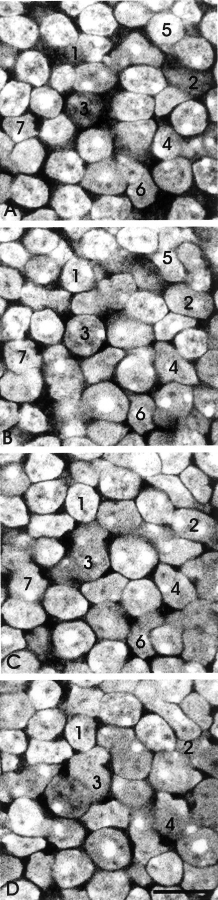
Serial confocal sections at 1 μmz intervals through the inner nuclear layer. All nuclei of the layer were labeled with ethidium homodimer. The cells were counted by following individual cells through the series, as illustrated for the numbered examples. Scale bar, 10 μm.

The average density of neurons in the ganglion cell layer was ∼8200 cells/mm². Of these, ∼41%, or 3300 cells/mm², are indeed ganglion cells (see below). This gives an average ratio of cones to ganglion cells of slightly less than four.

Horizontal, bipolar, Müller, and amacrine cells

The high density of cells in the inner nuclear layer of the mouse, combined with their small size, made it necessary to use electron microscopy of serial sections to distinguish among the various cell types (Fig. 3). Cells were identified on the basis of the morphology and distribution of processes leaving from their somata. Cytological and positional features also helped in the identification. For instance, Müller cells display dark, elongated nuclei, which form an almost continuous layer separating the sclerally located bipolar and horizontal cells from amacrine cell somata, mostly positioned at the vitreal side of the inner nuclear layer.

Fig. 3.

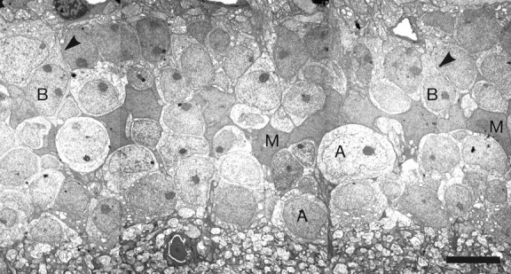
Low-power electron microscopy of the inner nuclear layer. Series of montages (part of one is shown) were assembled for locations in the central and peripheral retinas. Within each series of montages, every cell of the inner nuclear layer was identified. This was done by visualizing the axons or dendrites of the cells as they left the soma; examples are indicated by arrowheads. Scale bar, 5 μm.

Table 2 gives the numbers and relative fractions of various cell types in the inner nuclear layer. Bipolars make up ∼41% of all the cells in the layer, amacrines 39%, Müller cells 16%, and horizontal cells 3%. The size of the sample that one can examine with the electron microscope is obviously limited; this causes a considerable uncertainty in the estimate of fractions of horizontal cells, which are rarely encountered within the series of sections. The estimate for bipolars and amacrines is more accurate.

Table 2.

Distribution of major types of cells in the inner nuclear layer

	Central retina	Peripheral retina
Horizontal cells
Number of cells	8	10
Relative percentage	3	3
(Percentage estimated by dissector)	2	2
Bipolar cells
Number of cells	104	142
Relative percentage	40	43
(Percentage estimated by dissector)	41	43
Müller cells
Number of cells	40	52
Relative percentage	16	16
(Percentage estimated by dissector)	14	14
Amacrine cells
Number of cells	106	126
Relative percentage	41	38
(Percentage estimated by dissector)	43	41
Unidentified cells
Number of cells	none	4
Relative percentage		1
Total cells counted	258	334

As a cross-check, selected sections of the series were used to assess the same numbers and fractions by means of a widely used statistical sampling strategy, the dissector method (Gundersen, 1986). We found that a distance of 4 μm between the first and last section was suitable for applying the dissector method to the mouse inner nuclear layer. The results were close to those obtained by serial section analysis (Table 2). Although this was a useful exercise, note that using the dissector does not eliminate the need for an independent method of learning the identity of the partially sectioned cells.

Ganglion cells and displaced amacrine cells

We counted cells in the ganglion cell layer by staining another series of retinal whole mounts with ethidium homodimer and examining the preparations with a confocal microscope. All cells encountered in the samples were counted, with the exceptions of endothelial cells, clearly identified by their elongated shape and close association with blood vessels, and astrocytes, which have very small cell bodies with dense nuclei and are slightly displaced toward the optic fiber layer. Because we needed to determine the absolute number of ganglion cell layer neurons in the whole retina, we collected data from both the dorsoventral and the nasotemporal central meridians.

The distributions of total GCL neurons are shown in Figure4. The dorsoventral curves are not strictly symmetric to their nasotemporal counterparts. Because cells in the far periphery of the nasal retina have higher densities than for other peripheral regions, the center-to-periphery gradient for the nasal retina is lower than elsewhere. The total number of retinal cells in the layer was determined by multiplying the average density of cells in each retina by the total area of the retina. (A similar result was obtained by multiplying the measured local densities by the total area of the retina.)

Fig. 4.

Neurons of the ganglion cell layer. The top panel (A) shows a confocal image of the ganglion cell layer, as seen after staining with ethidium. Under these conditions both DNA and RNA are stained, so that extranuclear cytoplasm is revealed (arrows). The nuclei of glia and endothelial cells (arrowhead) were not counted. The two graphs (B, C) show the numbers of cells encountered along two axes (dorsoventral and nasotemporal) intersecting the optic nerve head. Counts are from the Italian colony of C57/BL6 mice.

The total number of ganglion cells was learned by counting their axons in the optic nerve, at a distance (∼300 μm) from the posterior pole of the eye in which most of them are myelinated and can be unequivocally identified at the electron microscope level (Fig.5). On average, 44,860 ± 3125 fibers were estimated (Table 3). Only 5% of them were clearly unmyelinated. For retinas with 110,242 ± 5826 neurons in the ganglion cell layer, 65,385 ± 6385 displaced amacrine cells thus exist, 59 ± 4% of the total.

Fig. 5.

Electron micrograph from transverse ultrathin section of the mouse optic nerve. Both large- and small-size axons are visible in this field, and all of them are myelinated. This magnification is approximately the same used for counting fibers.Nu, Nucleus of a glial cell. Scale bar, 1 μm.

Table 3.

Total ganglion cell layer neurons versus total optic nerve axons

Ganglion cell layer neurons
Retina	Neurons counted	Sampled area (μm2)	Mean density (cells/mm2)	Total retinal area (mm2)	Total GCL neurons
1	544	0.064	8540	13.4	114095
2	568	0.068	8280	15.2	125940
3	626	0.073	8517	15.5	131758
7	2632	0.470	5615	18.2	102140
8	3999	0.610	6565	17.7	115570
9	5277	0.690	6025	18.8	113020
Mean	2274	0.329	7257	16.5	117087

Optic nerve axons
Optic nerve	Axons counted	Sampled area (μm2)	Mean density (cells/mm2)	Total nerve area (mm2)	Total axons
7	5793	12303	0.47	92851	43720
10	5526	6345	0.87	54880	47800
11	5424	9676	0.56	71800	40248
12	6532	9676	0.68	70600	47660
Mean	5819	9500	0.65	72533	44857

ChAT (starburst) amacrine cells

As in other mammalian species, antibodies directed against choline acetyltransferase label two populations of virtually identical amacrine cells, whose cell bodies are located in the inner nuclear layer and ganglion cell layer, respectively, and whose dendrites form two narrow stratified bands within the inner plexiform layer. Confocal microscopy of the dendritic plexi labeled by anti-ChAT reveals the typical structure of starburst cell processes, with arbors that overlap to form a lattice pattern (Fig. 6).

Fig. 6.

The distribution of ChAT-positive (starburst) cells across three mouse retinas. In the top micrograph(A) the ChAT-positive neurons are, labeled here with Cy3, shown in red. They form two populations, one in the inner nuclear layer and one in the ganglion cell layer. Their dendrites are stratified narrowly in two bands. The middle micrograph (B) shows a collapsed whole-mount view. The ChAT cells of the inner nuclear layer arered, and those of the ganglion cell layer aregreen. The bottom micrograph(C) shows the mosaic of stained dendrites within the inner plexiform layer.

The numerical distribution of the two population of cells is quite symmetrical, with the cells in the inner nuclear layer reaching slightly higher densities at all eccentricities (on average, 1100 cells/mm² for inner nuclear layer cells vs 945 of the cells in the ganglion cell layer). The center-to-periphery gradient along the dorsoventral axis is two for the inner nuclear layer cells and slightly lower for the cells located in the ganglion cell layer.

The number of ChAT-positive cells can be compared with the total number of cells in the inner nuclear layer and ganglion cell layer learned by means of confocal microscopy (Table 1). ChAT cells with the cell bodies in the inner nuclear layer are ∼1% of all the cells in that layer. Since, in turn, 39% of all the inner nuclear layer cells are represented by amacrines, ChAT cells with the cell bodies in the inner nuclear layer are ∼3% of all amacrine cells. ChAT cells in the ganglion cell layer are 11.5% of all the cells in the layer, or 19.5% of all the displaced amacrines. The total population of ChAT cells (inner nuclear layer plus ganglion cell layer) represents 5.2% of the total number of amacrine cells in the mouse retina.

DISCUSSION

The distributions of each major cell type in the mouse retina are summarized in Figure 7. We find the mouse retina to be strongly rod-dominated: rods outnumber cones by roughly 35:1. Somewhat surprisingly, the average cone density in the mouse retina is the same found in the primate’s retina at 3–4 mm eccentricity (Packer et al., 1989). However, at the same eccentricity the density of rod photoreceptors in primates is only 100,000 cells/mm². Thus, the major difference between the photoreceptor mosaics of monkeys and mice is the higher density of (very small) rods in the latter.

In accord with the small overall size of the mouse eye, the cells of the inner nuclear layer are also small. Their average total density was 100,541 cells/mm², more than twice that in the rabbit (Strettoi and Masland, 1995). We find them distributed at 3.1% horizontal cells, 41% bipolars, 16% Müller cells, and 39% amacrine cells (Table 2). These fractions have previously been estimated from cytological features (Young, 1985). The corresponding values were 0.1, 48, 12 and 39%. The results are in fairly good agreement, with the exception that Young identified more bipolar and fewer Müller cells than we found. In our electron micrographs there is little ambiguity in distinguishing the two. It is likely that Young mistook some Müller cells for bipolars. This would be easy to do when the judgment is made purely from light microscopic cytology, because both cells can have vertically elongated somata and because the descending process of a Müller cell, which in the mouse is unusually thin, can resemble an axon of a bipolar cell.

The number of ganglion cells was very close to a previous computation done with similar methods in the same colony of animals, but almost 20% lower than that given in a careful study by Williams et al. (1996). The major difference between our counting strategy and theirs is that we use a larger field to count fibers: we count a larger number of fibers in a lower number of nerves. It is not obvious that technical differences would produce a discrepancy in the results. Two other factors could contribute to the difference: variation in tissue processing and individual variability between the American and the Italian colonies of mice. Tissue shrinkage, however, which is the major variable affected by processing, would not account for a difference in the total number of cells per retina. The more likely is that the Italian colony has a lower number of ganglion cells. There is precedent for such a difference: Williams et al. (1996) demonstrated a 21% difference in the numbers of ganglion cells between two Jackson Laboratory (Bar Harbor, ME) colonies of C57BL/6J mice. Note that the absolute densities of cells in the ganglion cell layer of retinas used for optic nerve counting were consistently lower than for the whole mounts in which we counted photoreceptors and inner nuclear layer cells; the total number of cells in the ganglion cell layer was lower in Italian than American mice (110,000 vs 124,000).

It is worth noting that the number of retinal ganglion cells is quite variable in normal cats, monkeys, and humans (Illing and Wässle, 1981; Curcio and Allen, 1990; Spear et al., 1996). Ganglion cell number appears especially susceptible to small genetic or even environmental differences.

Fortunately, the difference in mice is only 11% and affects the absolute density but not the relative fraction of ganglion cells in the ganglion cell layer. That estimate was 41 ± 4%, obtained from animals of the same colony. In one case, the total number of cells in the ganglion cell layer and of fibers in the optic nerve was calculated for the same retina (this cannot be done routinely, because differing fixatives need to be used for whole mounts or electron microscopy). For that retina, the fraction of ganglion cells in the ganglion cell layer was 43%. If one takes the number of optic nerve fibers from Williams et al. (1996) (54,600) and the total number of ganglion cells from our American mice, the value is 44%. This is close to what we find, and within the limits of the error of any of these measurements.

A base of reference for future work

The absolute densities of the cells were quite reproducible from animal to animal for our series of identically prepared specimens (Table 1). When tissue preparation differs (in fixative, histochemical protocol, or coverslipping method) the variation will be greater because of variable shrinkage and/or distortion of the tissue. The absolute density may also vary with the age of the animal, because the mouse’s eye grows throughout early adult life without the addition of neurons. However, the relative fractions of cells are not subject to such influences. The retina is built of interlocking microcircuits whose individual elements must be present in the same ratios in order for the system to function properly. Previous work and the present studies agree that the fractions of horizontal, bipolar, Müller, and amacrine cells are remarkably constant from specimen to specimen and animal to animal (Strettoi and Masland, 1995).

For that reason, the results of the present studies can be used as a base of reference for future work. If mouse retinas are prepared as whole mounts in aqueous medium after light aldehyde fixation, the numbers of cells can be compared directly without gross error. If not, new data can be referred back to the present ones by using proportions. For example, the numerical importance of a newly stained type of bipolar cell can be learned if one establishes that cell’s fraction of the total cell population of the inner nuclear layer. From those data and the present ones the fraction of all bipolar cells occupied by the newly stained one can be directly calculated.

As a practical matter, we have provided the relative density of the ChAT-containing amacrines, a readily stained population for which good antibodies are available. These can be used as a reference population. For example, at location V7 (2.1 mm ventral to the optic nerve), the ChAT-positive cells had a density of 800 cells/mm². Using the information presented in Tables 1 and 2, one may calculate that this represents 2.4% of all amacrine cells or 2.1% of all bipolar cells present at that eccentricity. Thus, if a new cell and the ChAT cells are stained in the same preparation, the fraction of all inner nuclear layer cells or all bipolar or all amacrine cells occupied by the new cell can be approximated. This avoids the necessity of counting the total cells of the inner nuclear layer. Because small fractions are involved, however, the results are accurate only to a first approximation; for more precision the density of a new cell should be referred to counts of the total cells of the inner nuclear layer.

Perspectives on normal and genetically altered mice

Knowledge of the cell populations of the retina will be important as genetic techniques are used to alter retinal structures, because changing one element in the retinal network can have secondary effects on others. Cone deletion (Soucy et al., 1996) and ganglion cell overexpression (Bonfanti et al., 1996) are current examples. Even when no structures have been changed, however, the information is useful. Several examples, among many possible, follow.

Starburst amacrine cells in our whole mounts had a peak density in the inner nuclear layer of ∼1400 cells/mm². In the rabbit, however, their peak density is 800/mm². Does this suggest that the starburst cells have different functions in mice and rabbits? The present results show that starburst cells in mice represent 3% of all amacrine cells at that eccentricity, exactly the same fraction (3%) found in the rabbit (Strettoi and Masland, 1996). A postulated role of the dopaminergic amacrine cells is also strengthened. The present results allow the calculation that they represent only 0.08% of all amacrine cells, as would be expected for a cell widely believed to serve a neuromodulatory function (Masland et al., 1993; Gustincich et al., 1997).

Quantitative information is also important in interpreting developmental manipulations. In a now classic study, Turner et al. (1990) labeled retinal progenitor cells by retroviral injection. At the animal’s maturity, the retroviral marker was found to be present in all of the classes of retinal neuron. However, the distribution of labeled cells did not match the normal adult distribution shown here. For retinas labeled at embryonic day 13 (E13), the proportions of labeled cells in the inner nuclear layer were: horizontal cells 0.7%, bipolar cells 70%, Müller cells 6%, and amacrine cells 23%. In effect, there were far too many labeled bipolar cells and too few Müller and amacrine cells (Table 2). The sample of cells studied by Turner et al. was large enough to exclude chance variation as the cause. The mismatch does not affect their fundamental conclusion: that all cell classes can derive from E13 progenitors. One possibility would be that, contrary to the original belief (Turner et al., 1990), some Müller and amacrine cells have already become committed at E13. Another would be unequal expression or detection of the retrovirally inserted marker among the cell classes.

Are the retinas of lower mammals more complex than those of primates?

For many years the belief has existed that the retinas of lower animals are complex, carrying out sophisticated analyses of the visual input, whereas those of primates are simple, with more complex analyses deferred to their highly developed visual cortices. This may well be true for frogs and birds, which have remarkably complex retinas (Dubin, 1970; Dowling, 1987). Anatomy suggests, and electrophysiological experiments directly confirm, that frog retinas contain very sophisticated inner retinal mechanisms (Maturana et al., 1960). Among mammals, however, this is less clear. The types of bipolar and amacrine cells found thus far in rats, rabbits, cats, and monkeys are remarkably similar. This extends even to cells as anatomically distinctive as the starburst and AII amacrines (for review, see Wässle and Boycott, 1991).

If many individual elements are the same, how about the overall populations of bipolar and amacrine cells? Figure8 shows that these, too, are quite similar in the mouse, rabbit, and monkey. The monkey has more horizontal cells, and slightly fewer amacrine cells, but in no sense are monkey retinas “bipolar-dominated”. To be sure, the monkey fovea may be an exception; the comparison shown in Figure 8 is for a point 5 mm away from the fovea, chosen because the densities of cones was near that found in the mouse and rabbit. However, the fovea occupies <1% of the area of the monkey’s retina. Over most of its area, the cell populations in the monkey retina are similar to those of a mouse or rabbit.

Fig. 8.

The distribution of classes of cells in the mouse, rabbit, and monkey. Data for the mouse average the central and peripheral retinas. Data for the rabbit are from Strettoi and Masland (1995). Data for the monkey are from Martin and Grünert (1992).

Interestingly, the density of cones in the mouse retina is in the same order of magnitude as the density of cones in the monkey at 3–4 mm from the fovea (Table 1; Wikler and Rakic, 1990). It could be that cones, which appeared first during evolution (Okano et al., 1992;Goldsmith, 1994), dictated the major rules of retinal organization. Possibly a certain density of cones, common to monkeys and mice, brings with it populations of connected retinal neurons that remain in constant numerical proportions. After all, the only retinal cells exclusive to the rod pathway are rod bipolars. Since outside the fovea the density of cones is similar in monkeys and mice, cone bipolars are expected to be in close proportions in the two species, as well as the numerous types of cone-driven amacrine cells.

REFERENCES

- 1.Altman DG. Practical statistics for medical research. Chapman and Hall; New York: 1991. [Google Scholar]
- 2.Bevington PR, Robinson DK. Data reduction and error analysis for the physical science, 2nd Ed, pp 38–52. McGraw-Hill; New York: 1992. [Google Scholar]
- 3.Blanks JC, Johnson LV. Specific binding of peanut lectin to a class of retinal photoreceptor cells. Invest Ophthalmol Vis Sci. 1984;25:546–557. [PubMed] [Google Scholar]
- 4.Bonfanti L, Strettoi E, Chierzi S, Cenni MC, Liu X-H, Martinou J-C, Maffei L, Rabacchi SA. Protection of retinal ganglion cells from natural and axotomy-induced cell death in neonatal transgenic mice over-expressing bcl-2. J Neurosci. 1996;16:4186–4194. doi: 10.1523/JNEUROSCI.16-13-04186.1996. [DOI] [PMC free article] [PubMed] [Google Scholar]
- 5.Carter-Dawson LD, LaVail MM. Rods and cones in the mouse retina. J Comp Neurol. 1979;188:245–262. doi: 10.1002/cne.901880204. [DOI] [PubMed] [Google Scholar]
- 6.Cenni MC, Bonfanti L, Martinou J-C, Ratto GM, Strettoi E, Maffei L. Long term survival of retinal ganglion cells following optic nerve section in adult bcl-2 transgenic mice. Eur J Neurosci. 1996;8:1735–1745. doi: 10.1111/j.1460-9568.1996.tb01317.x. [DOI] [PubMed] [Google Scholar]
- 7.Chen J, Makino CL, Peachey NS, Baylor DA, Simon MI. Mechanisms of rhodopsin inactivation in vivo as revealed by a COOH-terminal truncation mutant. Science. 1995;267:374–377. doi: 10.1126/science.7824934. [DOI] [PubMed] [Google Scholar]
- 8.Curcio CA, Allen KA. Topography of ganglion cells in human retina. J Comp Neurol. 1990;300:5–25. doi: 10.1002/cne.903000103. [DOI] [PubMed] [Google Scholar]
- 9.Curcio CA, Packer O, Kalina RE. A whole mount method for sequential analysis of photoreceptor and ganglion cell topography in a single retina. Vision Res. 1987;27:9–15. doi: 10.1016/0042-6989(87)90137-4. [DOI] [PubMed] [Google Scholar]
- 10.Dowling JE. The retina: an approachable part of the brain. Belknap; Cambridge: 1987. [Google Scholar]
- 11.Dubin MW. The inner plexiform layer of the vertebrate retina: a quantitative and comparative electron microscopic analysis. J Comp Neurol. 1970;140:479–506. doi: 10.1002/cne.901400406. [DOI] [PubMed] [Google Scholar]
- 12.Goldsmith TH. Ultraviolet receptors and color vision: evolutionary implications and a dissonance of paradigms. Vision Res. 1994;34:1479–1487. doi: 10.1016/0042-6989(94)90150-3. [DOI] [PubMed] [Google Scholar]
- 13.Gundersen HJG. Stereology of arbitrary particles: a review of unbiased number and size estimators and the presentation of some new ones, in memory of William R. Thompson. J Microsc. 1986;143:3–45. [PubMed] [Google Scholar]
- 14.Gustincich S, Feigenspan A, Wu DK, Koopman LJ, Raviola E. Control of dopamine release in the retina: a transgenic approach to neural networks. Neuron. 1997;18:723–736. doi: 10.1016/s0896-6273(00)80313-x. [DOI] [PubMed] [Google Scholar]
- 15.Hughes A. The topography of vision in mammals of contrasting life style: comparative optics and retinal organisation. In: Crescitelli F, editor. Handbook of sensory physiology. Springer; Berlin: 1977. pp. 613–756. [Google Scholar]
- 16.Illing RB, Wässle H. The retinal projection to the thalamus in the cat: a quantitative investigation and a comparison with the retinotectal pathway. J Comp Neurol. 1981;202:265–285. doi: 10.1002/cne.902020211. [DOI] [PubMed] [Google Scholar]
- 17.Martin PR, Grunert U. Spatial density and immunoreactivity of bipolar cells in the macaque monkey retina. J Comp Neurol. 1992;323:269–287. doi: 10.1002/cne.903230210. [DOI] [PubMed] [Google Scholar]
- 18.Masland RH, Rizzo JF, III, Sandell JH. Developmental variation in the structure of the retina. J Neurosci. 1993;13:5194–5202. doi: 10.1523/JNEUROSCI.13-12-05194.1993. [DOI] [PMC free article] [PubMed] [Google Scholar]
- 19.Masu M, Iwakabe H, Tagawa Y, Miyoshi T, Yamashita M, Fukuda Y, Sasaki H, Hiroi K, Nakamura Y, Shigemoto R, Takada M, Nakamura K, Nakao K, Katsuki M, Nakanishi S. Specific deficit of the ON response in visual transmission by targeted disruption of the mGluR6 gene. Cell. 1995;80:757–765. doi: 10.1016/0092-8674(95)90354-2. [DOI] [PubMed] [Google Scholar]
- 20.Maturana HR, Lettvin JY, McCulloch WS, Pitts WH. Anatomy and physiology of vision in the frog (Rana Pipiens). J Gen Physiol. 1960;43:129–175. doi: 10.1085/jgp.43.6.129. [DOI] [PMC free article] [PubMed] [Google Scholar]
- 21.McNeil MA, Masland RH. Extreme diversity among amacrine cells: implications for function. Neuron. 1998;20:971–982. doi: 10.1016/s0896-6273(00)80478-x. [DOI] [PubMed] [Google Scholar]
- 22.Mitrofanis J, Vigny A, Stone J. Distribution of catecholaminergic cells in the retina of the rat, guinea pig, cat, and rabbit: independence from ganglion cell distribution. J Comp Neurol. 1988;267:1–14. doi: 10.1002/cne.902670102. [DOI] [PubMed] [Google Scholar]
- 23.Nirenberg SA, Meister M. The light response of retinal ganglion cells is truncated by a displaced amacrine circuit. Neuron. 1995;18:637–650. doi: 10.1016/s0896-6273(00)80304-9. [DOI] [PubMed] [Google Scholar]
- 24.Okano T, Kojima D, Fukada Y, Shichida Y. Primary structures of chicken cone visual pigments: vertebrate rhodopsins have evolved out of cone visual pigments. Proc Natl Acad Sci USA. 1992;89:5932–5936. doi: 10.1073/pnas.89.13.5932. [DOI] [PMC free article] [PubMed] [Google Scholar]
- 25.Packer O, Hendrickson AA, Curcio C. Photoreceptor topology in the retina of the adult pigtail macaque (Macaca nemestrina). J Comp Neurol. 1989;288:165–183. doi: 10.1002/cne.902880113. [DOI] [PubMed] [Google Scholar]
- 26.Soucy ER, Wang Y, Nathans J, Meister M. Ganglion cell response properties in the coneless retina of a transgenic mouse. Invest Ophthalmol Vis Sci [Suppl] 1996;37:1057. [Google Scholar]
- 27.Spear PD, Kim CBY, Ahmad A, Tom BW. Relationship between numbers of retinal ganglion cells and lateral geniculate neurons in the rhesus monkey. Vis Neurosci. 1996;13:199–203. doi: 10.1017/s0952523800007239. [DOI] [PubMed] [Google Scholar]
- 28.Sterio DC. The unbiased estimation of number and sizes of arbitrary particles using the dissector. J Microsc. 1984;134:127–136. doi: 10.1111/j.1365-2818.1984.tb02501.x. [DOI] [PubMed] [Google Scholar]
- 29.Strettoi E, Masland RH. The organization of the inner nuclear layer of the rabbit retina. J Neurosci. 1995;15:875–888. doi: 10.1523/JNEUROSCI.15-01-00875.1995. [DOI] [PMC free article] [PubMed] [Google Scholar]
- 30.Strettoi E, Masland RH. The number of unidentified amacrine cells in the rabbit’s retina. Proc Natl Acad Sci USA. 1996;93:14906–14911. doi: 10.1073/pnas.93.25.14906. [DOI] [PMC free article] [PubMed] [Google Scholar]
- 31.Szel A, Rohlich P, Caffe AR, Juliusson B, Aguirre G, vanVeen T. Unique topographic separation of two spectral classes of cones in the mouse retina. J Comp Neurol. 1992;325:327–342. doi: 10.1002/cne.903250302. [DOI] [PubMed] [Google Scholar]
- 32.Turner DL, Snyder EY, Cepko CL. Lineage-independent determination of cell type in the embryonic mouse retina. Neuron. 1990;4:833–845. doi: 10.1016/0896-6273(90)90136-4. [DOI] [PubMed] [Google Scholar]
- 33.Wässle H, Boycott BB. Functional architecture of the mammalian retina. Physiol Rev. 1991;71:447–480. doi: 10.1152/physrev.1991.71.2.447. [DOI] [PubMed] [Google Scholar]
- 34.Wikler KW, Rakic P. Distribution of photoreceptor subtypes in the retina of diurnal and nocturnal primates. J Neurosci. 1990;10:3390–3401. doi: 10.1523/JNEUROSCI.10-10-03390.1990. [DOI] [PMC free article] [PubMed] [Google Scholar]
- 35.Wikler KC, Szel A, Jacobsen A-L. Positional information and opsin identity in retinal cones. J Comp Neurol. 1996;374:96–107. doi: 10.1002/(SICI)1096-9861(19961007)374:1<96::AID-CNE7>3.0.CO;2-I. [DOI] [PubMed] [Google Scholar]
- 36.Williams RW, Strom RC, Rice DS, Goldowitz D. Genetic and environmental control of variation in retinal ganglion cell number in mice. J Neurosci. 1996;16:7193–7205. doi: 10.1523/JNEUROSCI.16-22-07193.1996. [DOI] [PMC free article] [PubMed] [Google Scholar]
- 37.Xu J, Dodd RL, Makino CL, Simon MI, Baylor DA, Chen J. Prolonged photoresponses in transgenic mouse rods lacking arrestin. Nature. 1997;389:505–509. doi: 10.1038/39068. [DOI] [PubMed] [Google Scholar]
- 38.Young RW. Cell differentiation in the retina of the mouse. Anat Rec. 1985;212:199–205. doi: 10.1002/ar.1092120215. [DOI] [PubMed] [Google Scholar]