Abstract
Solar radiation is a critical requirement for all solar power plants. As it is a time-varying quantity, the power output of any solar power plant is also time variant in nature. Hence, for the prediction of probable electricity generation for a few days in advance, for any solar power plant, forecasting solar radiation a few days into the future is vital. Hourly forecasting for a few days in advance may help a utility or ISO in the bidding process. In this study, 1-day-ahead to 6-day-ahead hourly solar radiation forecasting was been performed using the MARS, CART, M5 and random forest models. The data required for the forecasting were collected from a solar radiation resource setup, commissioned by an autonomous body of the Government of India in Gorakhpur, India. From the results, it was determined that, for the present study, the random forest model provided the best results, whereas the CART model presented the worst results among all four models considered.
Keywords: Electrical engineering, Energy, Applied computing, M5, CART, Global solar radiation forecasting, Mars, Random forest, Statistics, Radiation physics
Electrical engineering; Energy; Applied computing; M5; CART; Global solar radiation forecasting; Mars; Random forest; Statistics; Radiation physics
1. Introduction
Electricity is a very important element of modern urban and rural life. Rising demand and environmental considerations have prompted the examination of renewable solutions for energy production. Currently, renewable energy power sources have entered the picture and have received much attention from researchers and governments. Due to the intermittent nature of renewable energy resources, such methods are vulnerable to power imbalances [1]. Solar power is a very important source of renewable energy because of its sustainable and non-polluting nature, along with its abundance [2]. The main drawback of solar power is its variability, which is due to the intermittent nature of solar radiation. Solar radiation is a key indicator of solar energy availability. Hence, for power management, forecasting of solar radiation is very important. Forecasting helps a utility to predict how much electricity will be produced from a given plant in the upcoming hours or days [3]. This may help ISOs in making decisions regarding which peak-load plants need to be in operation and which may be put on standby. With this approach, generation costs may decrease and users may ultimately benefit financially [4]. Machine learning models are used for various types of forecasting and continue to produce improved forecasting results.
1.1. Solar radiation forecasting models
In recent years, many techniques have been developed for solar radiation prediction, and can be broadly classified into two broad categories, cloud imagery combined with physical models and machine learning models. The choice between these two is mainly based on the time horizon for which the forecasting is required. For the short term (up to 6 h-ahead), forecasting extrapolation and statistical processes using satellite images or ground-level measurements and sky images are generally suitable [5]. The numerical weather prediction (NWP) model is a combination of post-processing modules and real-time measurements or satellite data. The NWP model is suitable for forecasting up to two days ahead or beyond [6]. Time-series models (such as ARMA and SARMA) have also been used in various literature reports for solar radiation forecasting and provide suitable results, but the main drawback of these models is that they are not able to consider nonlinearity in the data.
Machine learning is a subfield of computer science. Machine learning models have various advantages over other types of models, and they can model nonlinearities in data and establish relationships between inputs and outputs without requiring prior information. Due to these advantages, machine learning models are used for classification and regression purposes. Due to this, various machine learning models have been used for solar radiation forecasting in recent years. Artificial neural networks (ANN), nearest neighbour neural networks (k-NN), support vector machines (SVM) and Markov chain models have been detailed in the literature [7, 8, 9, 10]. The regression tree and random forest models have been rarely used model types but show good results. A detailed comparison and performance of these models are available in [2]. Some important research work conducted by various researchers in this area is presented here:
Behrooz Keshtegar et al. [11] compared four machine learning models for solar radiation forecasting. The data were acquired over 391 months at the Adana and Antakya stations in Turkey. Various combinations of maximum temperature, minimum temperature, sunshine hours, wind speed and relative humidity were selected as input variables for various forecasting models. The MARS, M5Tree, RSM (response surface method) and kriging models were compared on the basis of various statistical indicators. From their analysis, the authors found that, for forecasting at the Adana station, the MARS model showed the best forecasting results among all models considered.
Lunche Wang et al. [12] presented two forecasting models for solar radiation forecasting at 21 stations in China. Seven methodological variables were taken as inputs to fit the adaptive-neuro-fuzzy inference systems (ANFIS) and M5 models. The models were examined for data forecasting for 21 stations. From the analysis, it was found that, for different stations, different models presented better results. For station number 51777, the M5 model provided the best forecasting results.
M. Zamo et al. [13] compared 6 machine learning models for forecasting the PV power generation for the next day for power plants in France. The machine learning models used were the binary regression tree model, the Bagging model, the random forest model, the boosting model, the support vector machine model and the generalized additive model. The authors used the R software for modelling. The root mean squared error (RMSE), mean absolute error (MAE) and mean bias error (MBE) are indicators which were used for selection of the best model. From the comparison, the author found that the random forest model provided the best results among all of the models analysed.
Geoffrey K.F. Tso [14] compared the regression tree, linear regression and the ANN models for forecasting electricity consumption in Hong Kong, China. Comparison of the models was conducted using the square root of the average squared error. From the comparison, it was found that the regression tree model provided the best results.
From the literature review, it was found that the MARS, M5, regression tree and random forest models presented better results than other machine learning models. It was also found that one to a few day-ahead forecasting with hourly granularity is useful for unit commitments, transmission scheduling, and day-ahead markets [15]. In this paper, forecasting of the 1-day-ahead to 6-day-ahead solar radiation levels has been achieved using four machine learning models using a 12-month dataset for Gorakhpur, a site that is situated in the northern region of India. Forecasting was accomplished using the MARS, M5, regression tree and random forest models, as they were found to provide the best results, as has been indicated in different publications. For modelling purposes, the statistical software R [16] and its associated packages were used in this paper.
This paper is divided into five sections; the second section is dedicated to the description of site locations and data structures. The third section focuses on various machine learning models and statistical indicators. In the fourth section, the results and a comparison of all four machine learning models studied are presented. The fifth section is dedicated to the conclusions and a discussion of outcomes from this study.
2. Study area
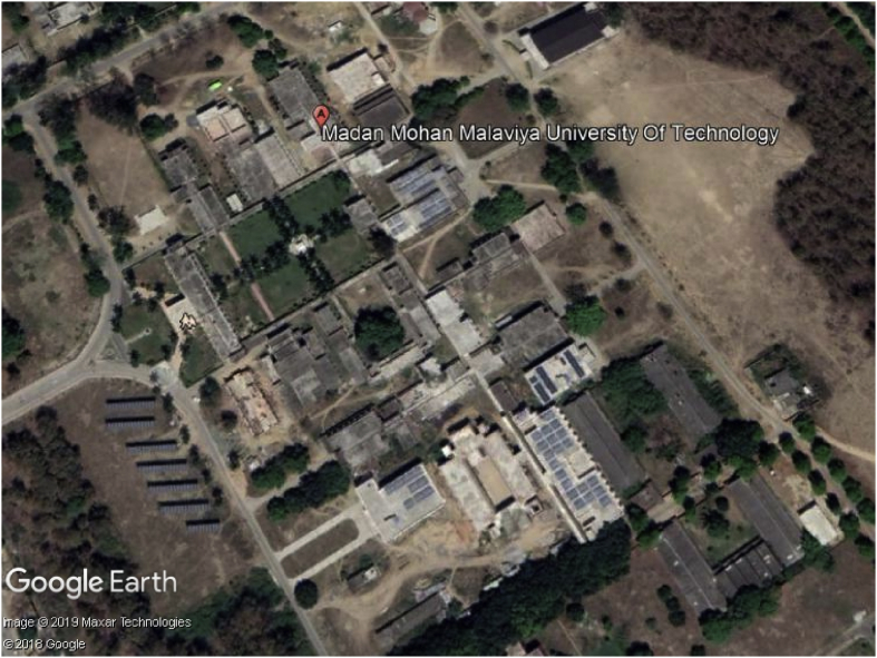
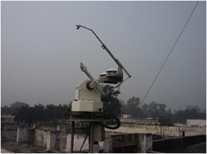
In this paper, solar radiation forecasting has been conducted for a site in Gorakhpur, India. Gorakhpur is located in the northern region of India and it is very close to Nepal. The mean annual temperature at Gorakhpur varies from 19.6 °C to 31.9 °C and the mean annual precipitation is 1,228.1 mm. The Madan Mohan Malaviya University of Technology (MMMUT) is a state university located in Gorakhpur. The solar radiation resources setup is located on the roof of the electrical engineering department of MMMUT, Gorakhpur. Site location of the setup is shown in Fig. 1. The setup is located at a latitude of 26°43′50.41″ N and a longitude of 83°26′2.8″ E. The altitude of the setup is 59 m above the sea level. A pictorial view of the setup is shown in Fig. 2. The setup was installed by the National Institute of Wind Energy (NIWE), an autonomous R&D institution that is under the Ministry of New and Renewable Energy (MNRE), Government of India [17]. The standards of the setup can be seen from [18].
Fig. 1.
Google earth image of the site location.
Fig. 2.
Pictorial view of the solar radiation resource setup.
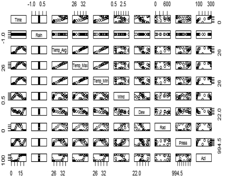
For the present study, one year (1st Jan 2017–31st Dec 2017) of data was collected using the setup shown. Nine data parameters were collected from the setup, namely minimum temperature (°C), maximum temperature (°C), average temperature (°C), wind speed (m/sec), rainfall (mm), dew point (°C), global solar radiation (W/m2), atmospheric pressure (mb), and solar azimuth (°). The setup collected the data in a minute-wise format but for proper fitting to the models, the minute-wise data were converted into hourly data. The temperature, wind, dew point, pressure and azimuth angle data were converted into hourly data by averaging the minute-wise data, whereas the rainfall and radiation data were converted into hourly data by summing the minute-wise data. 1-day, 2-day, 3-day, 4-day, 5-day, and 6-day-ahead forecasting were conducted in the present study. For this, the data from the earlier days of the month were used for model training, whereas the data from the latter days of the month were used for testing the models. For example, for 5-day-ahead forecasting in May, data from the 1st to 26th of May were used for model training and data from the 27th to 31st of May were used for model testing. Fig. 3 shows the data profile for the month of May.
Fig. 3.
Structure of data for the month of May.
3. Methodology
3.1. MARS model
The multivariate adaptive regression splines (MARS) algorithm was first introduced by Friedman in 1991 [19]. MARS is a nonlinear and nonparametric regression model. This model estimates the relationships between the dependent and independent variables by the use of piecewise linear splines. MARS simulates the model by the use of basic functions (BFs). BFs are defined in the form of pairs based on a knot to define an inflection region [20]. MARS generates a linear combination of BFs, which are shown below [19, 21]:
| (1) |
where, (j = 0, 1, 2…….n) are unknown coefficients and can be estimated by the least-square method, is a number of terms in the final model and can be estimated by the forward-backward stepwise process, andis jth basis function, which is given as:
| (2) |
where
The model is fitted based on n number of BFs that provides the lowest generalized cross-validation (GCV). The GCV can be formulated ass
| (3) |
where,
is the sum of square error andis the smoothing function.
The beauty of this model is that it does not require assumptions to establish a relationship between the input and output variables. In this model, the resulting piecewise curves enable greater flexibility because this model allows bends and thresholds which are not present in linear regression models. The MARS model fits in two stages, the first stage is the forward stage, in which functions are added and potential knots are detected to facilitate accuracy and to avoid an overfitted model. The second stage is the backward stage, in which the lower effective terms are eliminated. Details of the model can be seen in the work of Zhang and Goh [22].
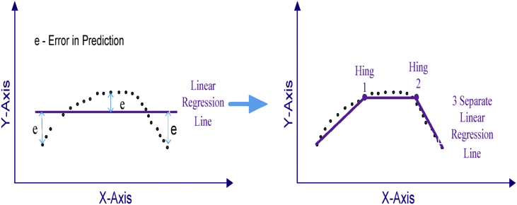
Fig. 4 shows an example of a MARS model. In this example, we can observe that if we apply a linear regression model to such data, the overall error (e) is quite high, but if we apply a MARS model containing 3 separate splines and 2 hinge functions, the resulting model has a lower overall error (e) and this matches the pattern of the data in more eloquent manner. The MARS model has been used in many applications in research, such as prediction modelling, financial management, and time series analysis [11, 23, 24]. In this paper, the MARS model was used for solar radiation forecasting.
Fig. 4.
Example of MARS model.
3.2. Classification and regression tree (CART)
The advantage of CART is that it is able to explore and highlight complex or hidden relationships in the data. The CART model is based on if-then rules. This is one of the most popular models used in machine learning for classification as well as for regression [25]. The CART model creates a single regression or classification tree by repeatedly splitting the data into groups by maintaining homogeneity in the output as much as possible using a set of decision rules that are applied to a specific explanatory variable [26]. The homogeneity in the output is measured through the residual sum of the squares, also known as the impurity of a node. First, the input variable is selected for splitting the node that maximizes the homogeneity in the child nodes that are related to the parent nodes, then other input variables are chosen as child nodes [27].
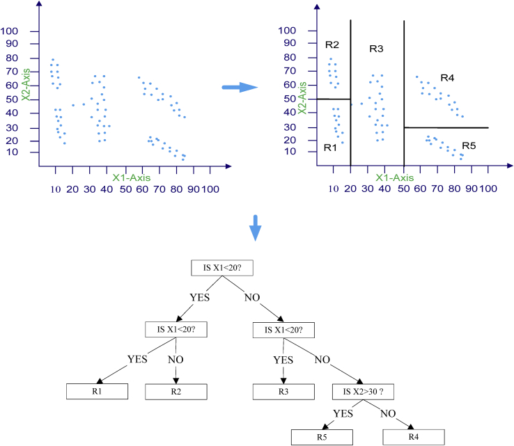
Once the optimal regression tree has been constructed, it is necessary to prune the tree to avoid overfitting. To select the optimal tree size, a cross-validation process is used. The cross-validation process helps to select the model with smallest prediction error. For better understanding, a simple example of the CART model is presented in Fig. 5, which shows the splitting of the input space X1×X2 (independent variables) into six subspaces (leaves) by the above-described algorithm.
Fig. 5.
Example of a Regression Model tree for splitting the Input Space X1×X2.
In addition, the CART model is widely used to solve regression problems in domains as diverse as engineering, medicine and the environment [28, 29, 30]. For example, A. Troncoso has used the CART model to predict wind speeds for a wind farm in northern Guadalajara, Spain [25]. Choi et al. used the CART model to predict air pollution levels for the south coast of California by using various meteorological variables as inputs to the model [31].
3.3. M5 model
The M5 model was first introduced by Quinlan in 1992 [32]. This model is based on a binary decision tree having linear regression functions at the terminal (leaf) nodes, and develops a relationship between the independent and dependent variables. The decision tree is only applicable for categorical data but this model can also be applied to quantitative data [33]. The M5 model uses two stages to fit the model. In the first stage, the data are split into subsets and form a decision tree. The splitting of the decision tree is based on treating the standard deviations of the class values that reach a node as measures of the error at the nodes and by calculating the expected reduction in this error as a result of testing each attribute at the node. The standard deviation can be calculated as:
| (4) |
where is a set of examples that reach the node, is the subset of examples that have the jth outcome of the potential set, and SD is the standard deviation.
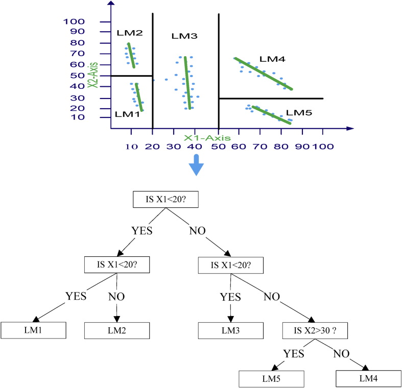
Due to the splitting, the standard deviation of a child node will be less than that of the parent node. After checking various splitting processes, the one that maximizes the expected error reduction is be chosen. The division tree has become overfitted. To overcome this overfitting, in the second stage, the overgrown tree is pruned and then the pruned sub-trees are replaced with linear regression functions [34, 35]. Fig. 6(a) shows the splitting of the input space X1×X2 (independent variables) into six subspaces (leaves) by the M5 model tree algorithm. Fig. 6(b) shows their relationships in the form of a tree diagram, in which LM1 to LM6 are at the leaf level.
Fig. 6.
Example of an M5 model tree, (a) Splitting the input space X1×X2 by the M5 model tree algorithm, (b) Diagram of the model tree with six linear regression nodes at the leaves.
The M5 tree model is analogous to the piecewise linear functions of regression trees. The advantage of the M5 model over the CART model is that the M5 model learns efficiently and can challenge and tackle problems having very high dimensionality and complexity. The M5 tree model is of smaller size than the CART model and its best trait is that the regression functions of the M5 model do not typically consist of many variables. The M5 model has also been used for many applications in recent years, such as engineering, medical and agricultural purposes. Recently, the M5 model has been successfully used for estimating reference evapotranspiration (ET0) [27], forecasting SO2 concentrations [36], pan evaporation modelling [37] and for daily river flow forecasting for the Sohu Stream, Turkey [38].
3.4. Random forest model
The random forest model is the most popular technique for regression and classification in decision tree learning. It is very efficient and, at the same time, its regression accuracy is better than the other regression methods. The random forest (RF) model was proposed by L. Breman in 1984 [39]. The random model constructs a large number of decorrelated decision trees in the training phase. After developing a number of decision trees, the output of the model is obtained by averaging the output values of all of the individual trees. For training any single tree, the learner bagging algorithm is used in the random forest model. Here, bagging repeatedly selects bootstrap samples of the training set and fits trees using the Gini impurity in these samples. After the training process, the predicted values for unseen examples are calculated by averaging the prediction results from all regression trees by:
| (5) |
By modelling different trees instead of a single tree, the random forest model presents better and more accurate predictions [14, 16]. The ranking of variables obtained with this methodology is unbiased and is more accurate than the CART results.
The random forest model is used in various classification and regression applications, such as estimations of metropolitan NO2 exposures in Japan [40], landslide susceptibility assessments in China [41], and mapping of groundwater potentials for Iranian [42] crop yield predictions [43].
3.5. Statistical indicators
All models were evaluated according to several comparison statistics, namely, the mean bias error (MBE), root mean squared error (RMSE) and the mean absolute error (MAE). The expressions for these criteria are given below:
| (6) |
| (7) |
| (8) |
where represents the error between the true value and the predicted value and n is the number of observations.
4. Results and discussion
1-day-ahead, 2-day-ahead, 3-day-ahead, 4-day-ahead, 5-day-ahead, and 6-day-ahead solar radiation forecasting was conducted for every month of 2017. The MARS, CART, M5 and random forecast machine learning models were used for this forecasting. To fit these models, nine parameters, namely, time, minimum temperature, maximum temperature, average temperature, wind speed, rainfall, dew point, atmospheric pressure and solar azimuth were taken as the input variables, and the global solar radiation was used as the output variable. These nine input variables were selected because they represent superior correction factors. The RMSEs were used to measure the deviations between the forecasted and actual values. The RMSE values represent the short-term performance of the model. Lower RMSEs indicate a more accurate model. The RMSE % is used to evaluate the performance of the model for different months with different levels of available solar radiation. The MBE provides long term correlations between the forecasted and actual values, term by term. The MBE is used to describe whether the model is under or overpredicted. A negative value for the MBE indicates that the model is underpredicted and a positive MBE indicates that the model is overpredicted. The ideal value for MBE is zero [44]. The MAE shows the absolute value of the MBE. Four models were evaluated on the basis of these three statistical indicators to observe the performances of these models under various forecasting conditions.
4.1. Performance of the MARS model
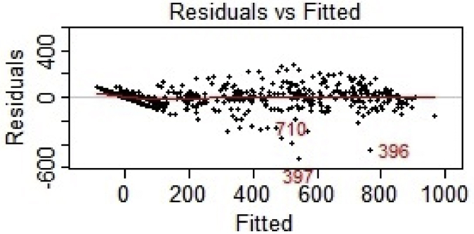
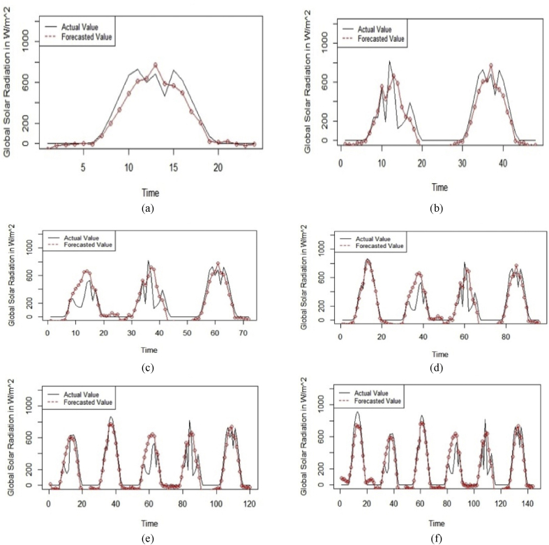
First, the MARS model was applied for 1-day-ahead to 6-day-ahead solar radiation forecasting. For fitting the MARS model, the “earth” package in the R software was used [45]. Fig. 7 presents a fitness vs. residual graph generated from the 1-day-ahead forecasting for May 2017. From Fig. 8, it can be observed that the model fits quite well and that the residuals are quite low. Fig. 8 presents the graph for (a) 1-day-ahead, (b) 2-day-ahead, (c) 3-day-ahead, (d) 4-day-ahead, (e) 5-day-ahead and (f) 6-day-ahead forecasted and actual values for May 2017. In this figure, the x-axis represents the hourly global solar radiation incidence at the surface in W/m2, and the y-axis represents time (in hours). From Fig. 8, it can be observed that this model shows good results, even for the 6-day-ahead forecasting.
Fig. 7.
MARS Model fitness graph for 1-day-ahead Forecasting on May Month.
Fig. 8.
(a) 1-day-ahead (b) 2-day-ahead (c) 3-day-ahead (d) 4-day-ahead (e) 5-day-ahead (f) 6-day-ahead Forecasted and Actual value graphs from the MARS Model for May 2017.
Table 1 is a matrix representation of the statistical errors in forecasting for various months and for various forecasting time spans. Table 1 shows that for 1-day-ahead forecasting, the lowest RMSE was seen for June, the highest RMSE was observed for January and the average RMSE for all months was 83.9%. For 2-day-ahead forecasting, the lowest RMSE was found in November, the highest RMSE was for January and the average RMSE for all months was 89.29%. For 3-day-ahead forecasting, the lowest RMSE was found for the month of October, the highest RMSE was found for May and the average RMSE for all months was 84.02%. For 4-day-ahead forecasting, the lowest RMSE was seen for October, the highest RMSE was found for January and the average RMSE for all months was 83.86%. For 5-day-ahead forecasting, the lowest RMSE was in October, the highest RMSE was in February and the average RMSE for all months was 83.39%. For 6-day-ahead forecasting, the lowest RMSE was for October, the highest RMSE was for January and the average RMSE for all months was 90.92%.
Table 1.
MARS model forecasting results.
| Jan | Feb | Mar | Apr | May | Jun | July | Aug | Sep | Oct | Nov | Dec | Avg | ||
|---|---|---|---|---|---|---|---|---|---|---|---|---|---|---|
| 1-day a-head | MBE | -39.86 | 106.66 | -4.81 | -32.55 | 35.60 | -8.97 | -0.70 | 38.81 | 22.19 | 20.11 | 3.64 | -11.16 | 10.75 |
| RMSE | 102.66 | 151.32 | 95.36 | 113.04 | 79.97 | 47.28 | 106.62 | 73.93 | 73.96 | 47.94 | 54.03 | 60.67 | 83.9 | |
| MAE | 70.45 | 106.66 | 59.65 | 50.96 | 58.69 | 39.21 | 63.36 | 50.34 | 53.94 | 37.30 | 42.60 | 45.42 | 56.55 | |
| 2-day a-head | MBE | 94.98 | 94.98 | 9.35 | -33.91 | 41.11 | -0.78 | -13.19 | -17.67 | -10.45 | 2.98 | 1.56 | -13.58 | 12.95 |
| RMSE | 143.30 | 143.30 | 67.02 | 101.79 | 123.54 | 66.94 | 94.48 | 89.05 | 78.66 | 48.48 | 46.98 | 67.97 | 89.29 | |
| MAE | 96.36 | 96.36 | 40.61 | 47.35 | 92.94 | 50.14 | 53.15 | 60.38 | 58.70 | 35.49 | 36.46 | 49.83 | 59.81 | |
| 3-day a-head | MBE | -19.38 | 80.80 | -1.94 | -23.12 | -4.79 | 6.28 | -14.09 | -39.46 | -13.04 | 9.91 | 17.22 | -4.91 | -0.54 |
| RMSE | 100.85 | 118.81 | 63.86 | 80.08 | 141.42 | 74.00 | 92.84 | 86.39 | 84.55 | 47.19 | 58.75 | 59.48 | 84.02 | |
| MAE | 63.67 | 83.89 | 38.90 | 46.01 | 99.89 | 49.29 | 54.53 | 60.96 | 69.46 | 36.08 | 44.61 | 44.56 | 57.65 | |
| 4-day a-head | MBE | 13.90 | 75.20 | -16.15 | -23.58 | 7.64 | 8.75 | 6.24 | -25.97 | -9.08 | 19.07 | 20.59 | 21.62 | 8.19 |
| RMSE | 110.73 | 119.00 | 66.26 | 79.30 | 125.15 | 78.60 | 82.41 | 80.12 | 91.54 | 48.01 | 61.49 | 63.75 | 83.86 | |
| MAE | 75.01 | 78.54 | 38.93 | 49.89 | 86.75 | 54.36 | 52.27 | 57.93 | 73.69 | 36.17 | 46.26 | 51.19 | 58.42 | |
| 5-day a-head | MBE | 5.24 | 69.29 | -22.07 | -15.47 | 6.48 | 15.14 | -24.18 | -18.33 | -5.41 | 22.31 | 25.98 | 2.28 | 5.11 |
| RMSE | 97.52 | 119.17 | 65.22 | 78.24 | 126.62 | 79.11 | 83.73 | 76.85 | 83.81 | 53.57 | 68.72 | 68.12 | 83.39 | |
| MAE | 65.15 | 74.39 | 36.98 | 53.53 | 85.68 | 58.45 | 54.86 | 57.27 | 65.35 | 40.44 | 49.90 | 51.51 | 57.79 | |
| 6-day a-head | MBE | -75.85 | 68.42 | -14.01 | 8.31 | 9.57 | 42.71 | -36.27 | -18.75 | 2.73 | 30.99 | 18.34 | 5.79 | 3.5 |
| RMSE | 174.53 | 121.04 | 61.64 | 74.43 | 117.99 | 101.88 | 87.30 | 72.13 | 94.99 | 55.60 | 66.45 | 63.07 | 90.92 | |
| MAE | 114.77 | 74.84 | 36.96 | 52.40 | 81.99 | 72.66 | 61.28 | 52.09 | 64.29 | 43.24 | 49.24 | 47.25 | 62.58 |
4.2. Performance of the CART model
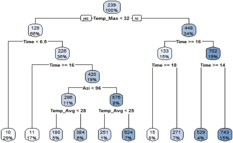
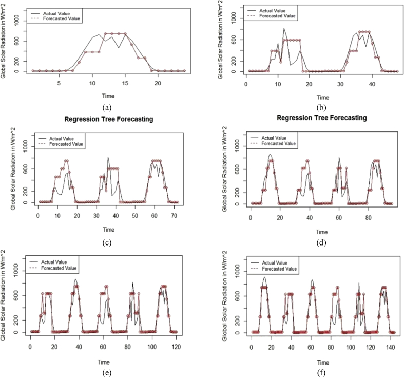
The classification and regression tree model is the basic decision tree model. To fit the MARS model, the “rpart” and “RWeka” packages of the R software were used [46, 47]. The CART model was applied for 1-day-ahead to 6-day-ahead solar radiation forecasting for all months of 2017. Fig. 9 represents the regression tree structure employed for 1-day-ahead forecasting for May. Fig. 10 presents (a) 1-day-ahead, (b) 2-day-ahead, (c) 3-day-ahead, (d) 4-day-ahead, (e) 5-day-ahead and (f) 6-day-ahead forecasting results for May 2017. The x-axis represents the hourly global solar radiation incidence on the surface in W/m2 and the y-axis represents time (in hours).
Fig. 9.
Regression Tree Structure used for 1-day-ahead Forecasting in May.
Fig. 10.
(a) 1-day-ahead (b) 2-day-ahead (c) 3-day-ahead (d) 4-day-ahead (e) 5-day-ahead (f) 6-day-ahead Forecasted and Actual value graphs from the CART Model for May 2017.
Table 2 shows a matrix representation of the various statistical errors observed from the 1-day-ahead to 6-day-ahead forecasting in various months. From Table 2, it can be observed that for the 1-day-ahead forecasting, the lowest RMSE was seen in December, the highest RMSE was observed for May and average RMSE for all months was 93.04%. For 2-day-ahead forecasting, the lowest RMSE was in November, the highest RMSE was in July and the average RMSE for all months was 93.24%. For 3-day-ahead forecasting, the lowest RMSE was in January, the highest RMSE was in July and the average RMSE for all months was 90.84%. For 4-day-ahead forecasting, the lowest RMSE was observed for January, the highest RMSE was seen in May and the average RMSE for all months was 92.91%. For 5-day-ahead forecasting, the lowest RMSE was seen in October. The highest RMSE was in May and the average RMSE for all months was 94.87%. For 6-day-ahead forecasting, the lowest RMSE was observed in October, the highest RMSE was found in January and the average RMSE for all months was 103.92%.
Table 2.
CART model forecasting results.
| Jan | Feb | Mar | Apr | May | Jun | July | Aug | Sep | Oct | Nov | Dec | Avg | ||
|---|---|---|---|---|---|---|---|---|---|---|---|---|---|---|
| 1-day a-head | MBE | -14.49 | 32.23 | 0.94 | -32.59 | 22.21 | 16.57 | -12.21 | 17.23 | 70.92 | 37.01 | 11.65 | -12.56 | 11.41 |
| RMSE | 51.79 | 117.69 | 97.35 | 121.56 | 123.02 | 62.51 | 114.84 | 73.58 | 136.76 | 111.81 | 59.93 | 45.63 | 93.04 | |
| MAE | 29.77 | 76.22 | 59.58 | 73.15 | 76.57 | 43.06 | 68.26 | 46.29 | 77.57 | 69.93 | 28.71 | 25.74 | 56.24 | |
| 2-day a-head | MBE | -16.81 | 31.38 | 17.63 | -16.78 | -12.09 | 18.34 | 22.71 | -37.75 | 46.75 | 21.49 | 29.51 | -15.13 | 7.44 |
| RMSE | 66.25 | 69.93 | 84.80 | 98.14 | 154.35 | 80.71 | 135.07 | 111.17 | 108.20 | 67.06 | 83.58 | 59.63 | 93.24 | |
| MAE | 35.37 | 41.61 | 51.59 | 58.87 | 93.62 | 54.52 | 69.76 | 65.11 | 61.39 | 46.78 | 46.78 | 31.83 | 54.77 | |
| 3-day a-head | MBE | -11.79 | 21.04 | -5.54 | 5.72 | -50.33 | 19.25 | -1.16 | -27.45 | 36.14 | 28.10 | 24.20 | -10.61 | 2.3 |
| RMSE | 60.23 | 54.50 | 100.58 | 95.04 | 159.28 | 81.38 | 118.60 | 102.13 | 94.88 | 94.85 | 74.39 | 54.21 | 90.84 | |
| MAE | 33.21 | 35.12 | 64.15 | 58.60 | 95.68 | 55.50 | 61.46 | 60.54 | 54.52 | 58.33 | 43.31 | 29.89 | 54.19 | |
| 4-day a-head | MBE | 11.12 | 34.66 | -13.36 | 9.08 | -10.62 | 36.40 | -2.96 | -20.46 | 38.96 | 27.74 | 23.54 | 4.11 | 11.52 |
| RMSE | 67.51 | 93.00 | 72.30 | 106.36 | 139.89 | 81.88 | 99.97 | 96.83 | 100.84 | 109.14 | 71.32 | 75.90 | 92.91 | |
| MAE | 40.83 | 59.97 | 45.73 | 65.59 | 81.36 | 56.77 | 59.97 | 58.56 | 58.56 | 67.37 | 43.06 | 45.42 | 56.93 | |
| 5-day a-head | MBE | -21.96 | 41.89 | -14.14 | 14.82 | -31.67 | 24.71 | 2.33 | -3.27 | 14.94 | 27.11 | 19.04 | -19.76 | 4.5 |
| RMSE | 107.64 | 100.11 | 68.69 | 104.13 | 135.60 | 84.00 | 92.21 | 103.36 | 98.32 | 60.78 | 86.66 | 96.88 | 94.87 | |
| MAE | 55.02 | 66.55 | 43.09 | 66.22 | 76.20 | 57.93 | 54.84 | 63.10 | 57.14 | 38.68 | 49.00 | 49.52 | 56.44 | |
| 6-day a-head | MBE | -16.74 | 39.17 | -46.56 | 17.75 | -20.64 | 35.96 | -4.91 | -2.00 | 9.95 | 23.15 | 16.70 | -15.06 | 3.06 |
| RMSE | 112.93 | 107.71 | 120.36 | 103.74 | 128.06 | 83.65 | 108.68 | 104.24 | 116.94 | 59.95 | 99.14 | 101.63 | 103.92 | |
| MAE | 64.30 | 74.28 | 84.96 | 67.29 | 72.63 | 56.59 | 59.85 | 61.29 | 67.15 | 38.63 | 54.93 | 57.87 | 63.31 |
4.3. Performance of the M5 model
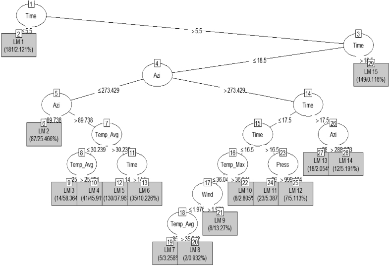
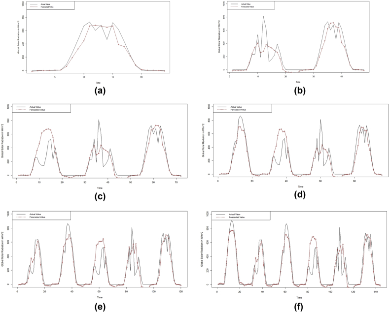
M5 is a modified version of the CART model and is also known as the leaf regression tree model. For modelling with the M5 model, the “rpart” and “RWeka” packages of R software were used [46, 47]. The M5 model was employed for 1-day-ahead to 6-day-ahead solar radiation forecasting. Fig. 11 represents the regression tree structure generated for the M5 model fitting for 1-day-ahead forecasting in May. Fig. 12 represents 1-day-head to 6-day-ahead forecasted and actual results for May. The axis labels are the same as those in Fig. 9.
Fig. 11.
Tree structure used for 1-day-ahead forecasting in May with the M5 Model.
Fig. 12.
(a) 1-day-ahead (b) 2-day-ahead (c) 3-day-ahead (d) 4-day-ahead (e) 5-day-ahead (f) 6-day-ahead forecasted and actual value graphs for the M5 model for May 2017.
Table 3 presents a matrix representation of the various errors observed in the 1-day-ahead to 6-day-ahead forecasting cases for various months. Table 3 shows that for 1-day-ahead forecasting, the lowest RMSE was in February, the highest RMSE was seen in the April and the average RMSE for all months was 70.15%. For 2-day-ahead forecasting, the lowest RMSE was in February, the highest RMSE was observed in August and the average RMSE for all months was 71.97%. For 3-day-ahead forecasting, the lowest RMSE was in February, the highest RMSE was in August and the average RMSE for all months was 76.71%. For 4-day-ahead forecasting, the lowest RMSE was observed for October, the highest RMSE was in May and the average RMSE for all months was 74.89%. For 5-day-ahead forecasting, the lowest RMSE was seen for November, the highest RMSE was in August and the average RMSE for all months was 76.11%. For 6-day-ahead forecasting, the lowest RMSE was in November, the highest RMSE was in July and the average RMSE for all months was 78.26%.
Table 3.
M5 model forecasting results.
| Jan | Feb | Mar | Apr | May | Jun | July | Aug | Sep | Oct | Nov | Dec | Avg | ||
|---|---|---|---|---|---|---|---|---|---|---|---|---|---|---|
| 1-day a-head | MBE | -19.40 | -5.06 | -15.18 | -46.18 | 26.95 | -26.74 | -4.72 | 37.32 | -22.44 | -3.86 | 23.12 | -16.30 | -6.04 |
| RMSE | 35.70 | 30.15 | 113.80 | 126.31 | 86.87 | 51.70 | 118.54 | 89.96 | 58.33 | 41.38 | 57.55 | 31.52 | 70.15 | |
| MAE | 21.48 | 20.07 | 71.89 | 64.15 | 51.77 | 41.41 | 71.03 | 57.21 | 35.56 | 25.80 | 34.06 | 18.95 | 42.78 | |
| 2-day a-head | MBE | -32.01 | 2.87 | 2.87 | -36.00 | 30.34 | -3.31 | 13.72 | -46.20 | -27.33 | -2.60 | 14.58 | -28.81 | -9.32 |
| RMSE | 63.73 | 40.79 | 40.79 | 87.07 | 120.19 | 57.23 | 108.49 | 131.56 | 61.64 | 46.96 | 47.87 | 57.36 | 71.97 | |
| MAE | 38.93 | 25.48 | 25.48 | 42.05 | 72.47 | 43.40 | 61.40 | 80.97 | 38.18 | 30.28 | 27.61 | 35.04 | 43.44 | |
| 3-day a-head | MBE | -22.86 | 11.98 | 9.47 | -34.80 | -17.08 | 4.33 | -6.97 | -60.73 | -17.51 | -2.01 | -0.61 | -20.58 | -13.11 |
| RMSE | 56.88 | 45.99 | 84.77 | 79.45 | 146.73 | 57.95 | 96.47 | 131.58 | 52.29 | 52.81 | 64.45 | 51.19 | 76.71 | |
| MAE | 35.87 | 28.52 | 47.90 | 43.79 | 85.07 | 41.89 | 54.43 | 81.65 | 34.84 | 34.22 | 38.46 | 32.28 | 46.58 | |
| 4-day a-head | MBE | 0.02 | 23.91 | -4.81 | -30.44 | 4.42 | 10.64 | -33.85 | -53.85 | -13.03 | -6.17 | 1.16 | 5.86 | -8.01 |
| RMSE | 52.32 | 60.07 | 64.27 | 74.04 | 129.39 | 65.38 | 99.03 | 120.78 | 59.13 | 51.86 | 62.30 | 60.11 | 74.89 | |
| MAE | 31.13 | 34.24 | 38.27 | 42.02 | 75.09 | 46.54 | 59.40 | 75.36 | 40.77 | 33.90 | 38.13 | 36.47 | 45.94 | |
| 5-day a-head | MBE | -27.30 | 25.47 | -9.32 | -17.94 | 0.68 | 6.56 | -40.43 | -47.72 | -11.80 | -4.16 | 7.39 | -24.57 | -11.93 |
| RMSE | 81.23 | 64.91 | 59.92 | 66.19 | 124.02 | 67.36 | 97.46 | 114.28 | 55.67 | 54.79 | 54.34 | 73.10 | 76.11 | |
| MAE | 48.57 | 37.26 | 36.09 | 37.84 | 75.29 | 48.86 | 62.84 | 67.27 | 39.82 | 35.69 | 34.48 | 43.71 | 47.31 | |
| 6-day a-head | MBE | -26.47 | 15.69 | -20.14 | -2.80 | -1.50 | -3.93 | -46.06 | -37.71 | -11.27 | -0.07 | 7.11 | -23.82 | -12.58 |
| RMSE | 77.52 | 61.16 | 67.41 | 72.12 | 119.92 | 58.78 | 105.44 | 123.45 | 65.34 | 58.17 | 60.02 | 69.77 | 78.26 | |
| MAE | 46.06 | 37.62 | 43.55 | 46.13 | 70.80 | 44.85 | 68.31 | 71.03 | 45.76 | 37.56 | 37.74 | 41.45 | 49.24 |
4.4. Performance of the random forest model
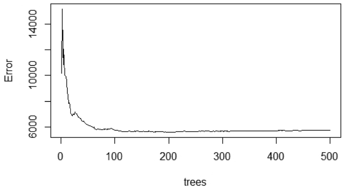
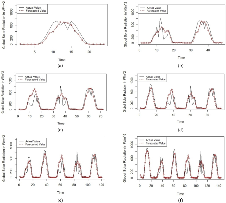
The random forest model is also a modified regression tree model, in which many regression trees are pruned in place of a single regression tree and the result is obtained by averaging all trees. 1-day-ahead to 6-day-ahead solar radiation forecasting was conducted for all months of 2017 using of the random forest model. For the regressions, the “randomForest” package of the R software was used [48]. For 1-day-ahead solar radiation forecasting in the month of May, a total of 500 trees were pruned. A graph of the errors and the numbers of trees is shown in Fig. 13. Fig. 13 shows that, by increasing the number of trees, the errors decrease but after including a sufficient number of trees, the graph flattens out. Fig. 14 depicts a graph showing the actual and forecasted values for 1-day-ahead to 6-day-ahead solar radiation forecasting for May.
Fig. 13.
Error vs. Number of Regression Tree Graph.
Fig. 14.
(a) 1-day-ahead (b) 2-day-ahead (c) 3-day-ahead (d) 4-day-ahead (e) 5-day-ahead (f) 6-day-ahead Forecasted and Actual value graph from the Random Forest Model for May 2017.
Table 4 shows a matrix representation of the various errors observed from 1-day-ahead to 6-day-ahead forecasting in various months. Table 4 shows that for 1-day-ahead forecasting, the lowest RMSE was in December, the highest RMSE was seen in April and the average RMSE of 62.88% was observed for the remaining months. For 2-day-ahead forecasting, the lowest RMSE was in October, the highest RMSE was in May and the average RMSE for the remaining months was 66.4%. For 3-day-ahead forecasting, the lowest RMSE was in October, the highest RMSE was observed for May and the average RMSE for all months was approximately 65.08%. For 4-day-ahead forecasting, the lowest RMSE was in January, the highest RMSE was observed for May and the average RMSE for all months was 60.38%. For 5-day-ahead forecasting, the lowest RMSE was in March, the highest RMSE was in May and the average RMSE for all months was 72.65%. For 6-day-ahead forecasting, the lowest RMSE was seen in October, the highest RMSE was in May and the average RMSE for all months was 78.77%.
Table 4.
Forecasting results with random forest model.
| Jan | Feb | Mar | Apr | May | Jun | July | Aug | Sep | Oct | Nov | Dec | Avg | ||
|---|---|---|---|---|---|---|---|---|---|---|---|---|---|---|
| 1-day a-head | MBE | -9.20 | 12.20 | -6.10 | -21.44 | 39.02 | -9.17 | 17.55 | 28.84 | 13.92 | 27.80 | 12.53 | -6.66 | 8.27 |
| RMSE | 24.46 | 26.50 | 93.98 | 118.01 | 104.65 | 34.00 | 117.46 | 59.28 | 58.67 | 48.83 | 46.30 | 22.47 | 62.88 | |
| MAE | 15.74 | 16.90 | 59.97 | 54.92 | 67.69 | 25.47 | 66.26 | 32.61 | 32.26 | 29.57 | 27.42 | 14.42 | 36.94 | |
| 2-day a-head | MBE | -23.13 | 20.25 | 17.72 | -16.06 | 16.36 | 2.54 | 21.19 | -30.02 | -9.04 | 7.45 | -1.92 | -20.11 | -1.23 |
| RMSE | 55.12 | 40.27 | 91.04 | 90.73 | 120.04 | 31.16 | 112.95 | 92.01 | 56.75 | 16.12 | 40.69 | 49.91 | 66.4 | |
| MAE | 28.14 | 26.01 | 61.28 | 41.92 | 73.50 | 21.91 | 60.48 | 50.53 | 35.16 | 9.84 | 27.31 | 25.43 | 38.46 | |
| 3-day a-head | MBE | -18.97 | 22.64 | 4.96 | -6.61 | -22.97 | 11.84 | 4.71 | -39.51 | -7.80 | 7.01 | 0.04 | -16.78 | -5.12 |
| RMSE | 53.25 | 44.80 | 81.63 | 76.05 | 133.85 | 48.16 | 94.67 | 93.76 | 52.76 | 16.62 | 39.06 | 46.32 | 65.08 | |
| MAE | 30.51 | 27.55 | 54.59 | 35.38 | 82.85 | 29.35 | 51.59 | 54.40 | 33.95 | 9.70 | 27.06 | 26.97 | 38.66 | |
| 4-day a-head | MBE | 0.95 | 28.55 | -3.89 | -0.21 | -0.80 | 21.73 | -25.55 | -30.40 | -1.51 | 11.51 | 0.47 | 0.47 | 0.11 |
| RMSE | 24.82 | 52.92 | 29.25 | 69.21 | 121.94 | 64.79 | 95.63 | 83.82 | 65.74 | 26.62 | 35.67 | 54.19 | 60.38 | |
| MAE | 13.63 | 32.66 | 18.15 | 35.62 | 76.43 | 40.68 | 58.77 | 49.86 | 40.67 | 15.17 | 23.70 | 30.88 | 36.35 | |
| 5-day a-head | MBE | -38.45 | 34.55 | -4.58 | 8.42 | 6.19 | 20.91 | -23.42 | -23.43 | -4.44 | 20.56 | 2.20 | -34.45 | -3 |
| RMSE | 104.26 | 64.72 | 27.13 | 68.60 | 118.39 | 67.24 | 88.75 | 87.07 | 62.89 | 39.20 | 49.76 | 93.80 | 72.65 | |
| MAE | 60.31 | 41.01 | 16.54 | 39.29 | 75.72 | 43.25 | 55.04 | 53.90 | 40.18 | 22.65 | 32.81 | 54.21 | 44.58 | |
| 6-day a-head | MBE | -30.21 | 32.95 | -35.30 | 28.01 | 5.89 | 23.75 | -22.20 | -23.94 | -7.70 | 26.15 | -1.66 | -26.98 | -2.6 |
| RMSE | 96.50 | 67.47 | 90.14 | 86.50 | 109.43 | 67.72 | 90.44 | 81.30 | 65.85 | 48.85 | 54.88 | 86.17 | 78.77 | |
| MAE | 52.97 | 46.81 | 61.54 | 54.45 | 68.07 | 44.33 | 54.90 | 51.69 | 42.04 | 29.47 | 35.22 | 47.86 | 49.11 |
4.5. Comparison of various models
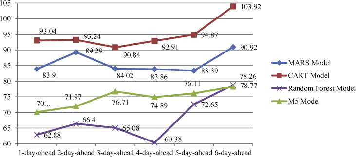
In this section, a comparison of the forecasting outcomes obtained from the different models is made. All four models were compared on the basis of their average RMSEs generated during the 1-day-ahead to 6-day-ahead solar radiation forecasting scenarios. The root mean square error (RMSE) value is the most significant statistical indicator for regression. Averaging of the results was done in such a way that, for generating the average RMSEs for 1-day-ahead forecasting, the results of the 1-day-ahead forecasting in the months of January to December were averaged. Fig. 15 shows the average RMSE graph for the forecasting outcomes as obtained from the various models considered. Fig. 15 shows that, in all cases, the random forest model produced the lowest RMSEs, the M5 model produced the second lowest RMSEs, the MARS model produced the third lowest RMSEs and the CART model produced the greatest RMSEs.
Fig. 15.
Comparison of the MARS, regression tree, M5 and random forest models.
We conclude that in this case study, the random forest model produced the best results among all models considered. The M5 model generated better results than the MARS and CART models. The MARS model produced better results than the CART model and inferior results compared to the M5 and random forest models. The CART model had the worst results among all models considered.
4.6. Validation of results
Although these statistical errors are sufficient to compare the performances of the various models, they do not indicate whether the forecasted results were statistically significant. The t-static error provides information of whether the results are at a significant confidence level. The t-static error is formulated as:
| (9) |
Lower t-static errors mean better model performances. The standard t-table provides the standard t-static error values (tα/2 at α level of significance and (n-1) degrees of freedom) to check the significance of the results. Those models that presented lower t (calculated) values than the standard t (tabulated) values are statistically significant [49].
Table 5 presents the t-static errors from the various models and the standard critical t-static values at the 95% confidence level. Table 5 shows that all models presented lower t-static errors than the standards in all cases. This means that all results were statistically significant. It can also be observed that in the months of January, February and December (winter season), the t-static errors were higher because, in the northern region of India, fog deposition is high and the availability of solar radiation is lower and naturally varies.
Table 5.
t-static Errors from the Various Models and the Standard t-static Error Values.
| Jan | Feb | Mar | Apr | May | Jun | July | Aug | Sep | Oct | Nov | Dec | Standard t-static error values at 95% confidence level [50] | |
|---|---|---|---|---|---|---|---|---|---|---|---|---|---|
| MARS Model | |||||||||||||
| 1 Day a-head | 1.114 | -1.647 | 0.059 | 0.412 | -0.438 | 0.101 | 0.009 | -0.516 | -0.289 | -0.242 | -0.066 | 0.414 | 2.069 |
| 2 Day a-head | 1.508 | -1.892 | -0.163 | 0.547 | -0.762 | 0.012 | 0.273 | 0.330 | 0.201 | -0.049 | -0.041 | 0.626 | 2.013 |
| 3 Day a-head | 0.772 | -1.874 | 0.043 | 0.450 | 0.113 | -0.123 | 0.381 | 0.892 | 0.317 | -0.203 | -0.570 | 0.227 | 1.994 |
| 4 Day a-head | -0.577 | -1.908 | 0.416 | 0.518 | -0.195 | -0.197 | -0.193 | 0.686 | 0.258 | -0.449 | -0.793 | -0.924 | 1.984 |
| 5 Day a-head | -0.241 | -1.918 | 0.633 | 0.382 | -0.190 | -0.385 | 0.783 | 0.548 | 0.177 | -0.586 | -1.157 | -0.111 | 1.98 |
| 6 Day a-head | -0.859 | -1.965 | 0.431 | -0.232 | -0.298 | -1.251 | 1.328 | 0.631 | -0.096 | -0.892 | -0.900 | -0.294 | 1.976 |
| M5 | |||||||||||||
| 1 Day a-head | 0.851 | 0.066 | 0.201 | 0.592 | -0.333 | 0.294 | 0.064 | -0.507 | 0.271 | 0.047 | -0.433 | 0.817 | 2.069 |
| 2 Day a-head | 1.510 | -0.052 | -0.270 | 0.600 | -0.608 | 0.052 | -0.311 | 1.285 | 0.484 | 0.043 | -0.385 | 1.510 | 2.013 |
| 3 Day a-head | 1.014 | -0.271 | -0.228 | 0.668 | 0.421 | -0.084 | 0.205 | 1.285 | 0.389 | 0.041 | 0.019 | 1.014 | 1.994 |
| 4 Day a-head | -0.001 | -0.634 | 0.134 | 0.664 | -0.121 | -0.239 | 1.037 | 1.325 | 0.342 | 0.148 | -0.042 | -0.276 | 1.984 |
| 5 Day a-head | 1.238 | -0.745 | 0.288 | 0.440 | -0.021 | -0.239 | 1.316 | 1.293 | 0.360 | 0.110 | -0.312 | 1.238 | 1.98 |
| 6 Day a-head | 1.255 | -0.486 | 0.657 | 0.077 | 0.047 | 0.109 | 1.642 | 1.188 | 0.386 | 0.002 | -0.335 | 1.255 | 1.976 |
| Random Forest Model | |||||||||||||
| 1 Day a-head | 0.395 | -0.161 | 0.081 | 0.275 | -0.488 | 0.101 | -0.246 | -0.376 | -0.182 | -0.339 | -0.227 | 0.377 | 2.069 |
| 2 Day a-head | 1.162 | -0.369 | -0.340 | 0.271 | -0.329 | -0.039 | -0.493 | 0.541 | 0.165 | -0.119 | 0.049 | 1.124 | 2.013 |
| 3 Day a-head | 0.839 | -0.518 | -0.121 | 0.130 | 0.573 | -0.228 | -0.144 | 0.541 | 0.175 | -0.140 | -0.001 | 0.829 | 1.994 |
| 4 Day a-head | -0.039 | -0.756 | 0.106 | 0.005 | 0.022 | -0.486 | 0.802 | 0.764 | 0.040 | -0.269 | -0.017 | -0.022 | 1.984 |
| 5 Day a-head | 1.721 | -1.015 | 0.139 | -0.209 | -0.198 | -0.530 | 0.787 | 0.671 | 0.138 | -0.538 | -0.095 | 1.709 | 1.98 |
| 6 Day a-head | 1.429 | -1.048 | 1.178 | -0.779 | -0.191 | -0.670 | 0.828 | 0.780 | 0.263 | -0.765 | 0.078 | 1.421 | 1.976 |
| Regression Tree Model | |||||||||||||
| 1 Day a-head | 0.620 | -0.423 | -0.012 | 0.427 | -0.269 | -0.187 | 0.156 | -0.215 | -1.010 | -0.456 | -0.204 | 0.617 | 2.069 |
| 2 Day a-head | 0.865 | -0.575 | -0.321 | 0.283 | 0.224 | -0.284 | -0.513 | 0.659 | -0.937 | -0.358 | -0.814 | 0.865 | 2.013 |
| 3 Day a-head | 0.510 | -0.477 | 0.124 | -0.114 | 1.171 | -0.372 | 0.034 | 0.593 | -0.859 | -0.584 | -0.794 | 0.510 | 1.994 |
| 4 Day a-head | -0.476 | -0.926 | 0.347 | -0.208 | 0.281 | -0.813 | 0.093 | 0.509 | -1.077 | -0.656 | -0.892 | -0.193 | 1.984 |
| 5 Day a-head | 0.954 | -1.240 | 0.411 | -0.374 | 0.925 | -0.611 | -0.080 | 0.093 | -0.456 | -0.724 | -0.818 | 0.954 | 1.98 |
| 6 Day a-head | 0.771 | -1.265 | 1.508 | -0.489 | 0.631 | -0.998 | 0.182 | 0.066 | -0.332 | -0.678 | -0.775 | 0.771 | 1.976 |
4.7. Discussion
A close examination of the results shows that all models presented good results. When viewing the differences between the 1-day-ahead forecasting results and the 6-day-ahead forecasting results, we observe that in the case of random forest forecasting, the differences between the RMSEs of the 1-day-ahead and the RMSEs of the 6-day-ahead forecasting were 15.89%, which were within acceptable limits. This shows that if we increase the day-ahead span for forecasting, acceptable results would be found. Moreover, a longer day-ahead forecasting period was beneficial. If we want to estimate the availability of solar radiation up to 6 days in advance, we can estimate its value accurately (within standard prescribed limits). These results can be useful for various applications, such as in solar power availability calculations, atmospheric energy-balance studies, analyses of the thermal loads on buildings, farming aspects and solar-dependent industries. For example, for power bidding by an ISO, a solar power plant must bid its rate and the amount of power to be injected into the grid at 1–6 days before on an hourly basis. The plant has a solar radiation measurement facility and can calculate the ratio by which the solar radiation is converted to available power. By having this information available, a plant can accurately predict values for solar power on an hourly basis. Hence, these results are very useful for power bidding up to 6 days before the power needs to be transmitted.
It can also be observed that the month is also a significant factor for forecasting in the northern region of India. In the summer season, clear solar radiation is available that the models were able to accurately predict. However, in the winter season, the solar radiation is lower and is non-uniform in nature; due to these factors, the models were not able to predict accurate results. In the rainy season, the maximum variations are sometimes seen when clear non-dusty skies are present, which facilitate high solar radiation that is otherwise available due to a cloudy atmosphere, for which low solar radiation is present; because of these effects, the models were not able to provide very good fits and contained lower prediction accuracies. In the northern region of India, in general, the winter season is from November to February, the summer season is from March to June and the rainy season is from July to October. In this paper, for the graphical representation of the actual and predicted values, the results for May were shown because of the maximum variations present in the actual solar radiation (This can be easily observed in the graph of actual values shown in Fig. 8), and if the models are able to fit in such variable data, then the model can easily fit the datasets for other months.
5. Conclusions
The performances of the CART, MARS, M5 and random forest models have been analysed for solar radiation forecasting in this case study. The model performances were examined on an hourly basis for 1-day-ahead to 6-day-ahead solar radiation forecasting for the site location at Gorakhpur, India. Forecasting was performed considering all months of 2017 so that the performance of forecasting could be evaluated in a more detailed manner. Nine metrological variables were taken as inputs to build the models and the results were compared through several comparative statistics, including the mean bias error (MBE), the root mean squared error (RMSE) and the mean absolute error (MAE). The outcomes of this case study are given below:
-
•
All four models provided sufficiently accurate results for 1-day-ahead to 6-day-ahead forecasting.
-
•
To check the feasibility of the results, t-static tests were also carried out. From the t-test errors, it was found that the results from the various forecasting models were statistically significant at the 95% confidence level.
-
•
When increasing the day-ahead span, the errors did not increase rapidly. Hence, these models were applicable for up to 6-day-ahead forecasting.
-
•
Forecasting errors were higher in the cloudy season because the variations in solar radiation were due more to clouds, whereas in the winter and summer seasons, the forecasting errors were low because the variations in solar radiation were lower due to the clear skies.
-
•
The order of the performance results is random forest > M5>MARS > CART (best to worst)
-
•
The results suggested that the random forest model can be used as an alternative to the CART, MARS, and M5Tree models for modelling solar radiation.
-
•
Hourly solar radiation forecasting will be helpful for estimations of the available solar power during every hour of the day. Such forecasting results are certainly beneficial for independent system operators (ISO) in their bidding processes.
Declarations
Author contribution statement
Rachit Srivastava: Conceived and designed the experiments; Performed the experiments; Wrote the paper.
A. N. Tiwari: Analyzed and interpreted the data.
V. K. Giri: Contributed reagents, materials, analysis tools or data.
Funding statement
The authors received no funding from an external source.
Competing interest statement
The authors declare no conflict of interest.
Additional information
No additional information is available for this paper.
References
- 1.Yang X., Xu M., Xu S., Han X. Day-ahead forecasting of photovoltaic output power with similar cloud space fusion based on incomplete historical data mining. Appl. Energy. 2017;206:683–696. [Google Scholar]
- 2.Voyant C. Machine learning methods for solar radiation forecasting: a review. Renew. Energy. 2017;105:569–582. [Google Scholar]
- 3.Espinar B., Aznarte J.L., Girard R., Moussa a.M., Kariniotakis G. vol. 33. 2010. Photovoltaic Forecasting: a state of the art; pp. 250–255. (5th Eur. PV-Hybrid Mini-Gird Conf.). [Google Scholar]
- 4.Kraas B., Schroedter-Homscheidt M., Madlener R. Economic merits of a state-of-the-art concentrating solar power forecasting system for participation in the Spanish electricity market. Sol. Energy. 2013;93:244–255. [Google Scholar]
- 5.Paulescu M., Paulescu E., Gravila P., Badescu V. Weather modeling and forecasting of PV systems operation. Green Energy Technol. 2013 [Google Scholar]
- 6.Perez R., Kivalov S., Schlemmer J., Hemker K., Renné D., Hoff T.E. Validation of short and medium term operational solar radiation forecasts in the US. Sol. Energy. 2010;84(12):2161–2172. [Google Scholar]
- 7.Marquez R., Coimbra C.F.M. Forecasting of global and direct solar irradiance using stochastic learning methods, ground experiments and the NWS database. Sol. Energy. 2011 [Google Scholar]
- 8.Moreno A., Gilabert M.A., Martínez B. Mapping daily global solar irradiation over Spain: a comparative study of selected approaches. Sol. Energy. 2011 [Google Scholar]
- 9.Ben Taieb S., Bontempi G., Atiya A.F., Sorjamaa A. A review and comparison of strategies for multi-step ahead time series forecasting based on the NN5 forecasting competition. Expert Syst. Appl. 2012 [Google Scholar]
- 10.Long H., Zhang Z., Su Y. Analysis of daily solar power prediction with data-driven approaches. Appl. Energy. 2014 [Google Scholar]
- 11.Keshtegar B., Mert C., Kisi O. Comparison of four heuristic regression techniques in solar radiation modeling: kriging method vs RSM, MARS and M5 model tree. Renew. Sustain. Energy Rev. 2018;81:330–341. [Google Scholar]
- 12.Wang L. Prediction of solar radiation in China using different adaptive neuro-fuzzy methods and M5 model tree. Int. J. Climatol. 2017;37(3):1141–1155. [Google Scholar]
- 13.Zamo M., Mestre O., Arbogast P., Pannekoucke O. A benchmark of statistical regression methods for short-term forecasting of photovoltaic electricity production, part I: deterministic forecast of hourly production. Sol. Energy. 2014;105:792–803. [Google Scholar]
- 14.Tso G.K.F., Yau K.K.W. Predicting electricity energy consumption: a comparison of regression analysis, decision tree and neural networks. Energy. 2007;32(9):1761–1768. [Google Scholar]
- 15.Kostylev V., Pavlovski A. 1st International Workshop on the Integration of Solar Power into Power Systems. Aarhus; Denmark: 2011. Solar power forecasting performance - towards industry standards. [Google Scholar]
- 16.Rs. Team . RStudio, Inc.; Boston, MA: 2016. “RStudio: Integrated Development for R,” [Online] RStudio, Inc., Boston, MA.http://www.rstudio.com URL. [Google Scholar]
- 17.(NIWE) National Institute of Wind Energy, “CWETSolar.” [Online]. Available: http://www.cwetsolar.com/. [Accessed: 28-Nov-2017].
- 18.Kumar A. Field experiences with the operation of solar radiation resource assessment stations in India. Energy Procedia. 2013;49:2351–2361. [Google Scholar]
- 19.Friedman J.H., Adaptive M., Splines R. Multivariate adaptive regression splines. Ann. Stat. 1991;19(1):1–67. [Google Scholar]
- 20.Mansouri I., Ozbakkaloglu T., Kisi O., Xie T. Predicting behavior of FRP-confined concrete using neuro fuzzy, neural network, multivariate adaptive regression splines and M5 model tree techniques. Mater. Struct. Constr. 2016;(–16):1. [Google Scholar]
- 21.Meyer H., Kühnlein M., Appelhans T., Nauss T. Comparison of four machine learning algorithms for their applicability in satellite-based optical rainfall retrievals. Atmos. Res. 2016;169:424–433. [Google Scholar]
- 22.Zhang W.G., Goh A.T.C. Multivariate adaptive regression splines for analysis of geotechnical engineering systems. Comput. Geotech. 2013 [Google Scholar]
- 23.Kisi O., Parmar K.S., Soni K., Demir V. Modeling of air pollutants using least square support vector regression, multivariate adaptive regression spline, and M5 model tree models. Air Qual. Atmos. Health. 2017;10(7):873–883. [Google Scholar]
- 24.Heddam S., Kisi O. Modelling daily dissolved oxygen concentration using least square support vector machine, multivariate adaptive regression splines and M5 model tree. J. Hydrol. 2018 [Google Scholar]
- 25.Troncoso A., Salcedo-Sanz S., Casanova-Mateo C., Riquelme J.C., Prieto L. Local models-based regression trees for very short-term wind speed prediction. Renew. Energy. 2015 [Google Scholar]
- 26.Arnett F.C. The american rheumatism association 1987 revised criteria for the classification of rheumatoid arthritis. Arthritis Rheum. 1988;31(3):315–324. doi: 10.1002/art.1780310302. [DOI] [PubMed] [Google Scholar]
- 27.Rahimikhoob A. Comparison between M5 model tree and neural networks for estimating reference evapotranspiration in an arid environment. Water Resour. Manag. 2014 [Google Scholar]
- 28.Tsiros I.X., Dimopoulos I.F., Chronopoulos K.I., Chronopoulos G. Estimating airborne pollutant concentrations in vegetated urban sites using statistical models with microclimate and urban geometry parameters as predictor variables: a case study in the city of Athens Greece. J. Environ. Sci. Health – Part A Toxic/Hazard. Subst. Environ. Eng. 2009 doi: 10.1080/10934520903263256. [DOI] [PubMed] [Google Scholar]
- 29.Aertsen W., Kint V., de Vos B., Deckers J., van Orshoven J., Muys B. Predicting forest site productivity in temperate lowland from forest floor, soil and litterfall characteristics using boosted regression trees. Plant Soil. 2012 [Google Scholar]
- 30.Juárez I., Mira-McWilliams J., González C. Important variable assessment and electricity price forecasting based on regression tree models: classification and regression trees, Bagging and Random Forests. IET Gener., Transm. Distrib. 2015 [Google Scholar]
- 31.Choi W., Paulson S.E., Casmassi J., Winer A.M. “Evaluating meteorological comparability in air quality studies: classification and regression trees for primary pollutants in California’s South Coast Air Basin. Atmos. Environ. 2013 [Google Scholar]
- 32.Quinlan J.R. Learning with continuous classes. Mach. Learn. 1992;92:343–348. [Google Scholar]
- 33.Mitchell T.M. 1997. Machine Learning. [Google Scholar]
- 34.Abdelkader S.S., Grolinger K., Capretz M.A.M. Proceedings - 2015 IEEE 14th International Conference on Machine Learning and Applications, ICMLA 2015. 2016. Predicting energy demand peak using M5 model trees; pp. 509–514. [Google Scholar]
- 35.Zhang X., Zhang X., Fang F. Chinese Control Conference. CCC; 2017. Power forecasting of solar photovoltaic power systems based on similar day and M5’ model trees; pp. 9238–9243. [Google Scholar]
- 36.Kisi O., Parmar K.S., Soni K., Demir V. Modeling of air pollutants using least square support vector regression, multivariate adaptive regression spline, and M5 model tree models. Air Qual. Atmos. Health. 2017 [Google Scholar]
- 37.Kisi O. Pan evaporation modeling using least square support vector machine, multivariate adaptive regression splines and M5 model tree. J. Hydrol. 2015 [Google Scholar]
- 38.Taghi Sattari M., Pal M., Apaydin H., Ozturk F. M5 model tree application in daily river flow forecasting in Sohu Stream, Turkey. Water Resour. 2013 [Google Scholar]
- 39.Breiman L. Random forest. Mach. Learn. 2001;45:5–32. [Google Scholar]
- 40.Araki S., Shima M., Yamamoto K. Spatiotemporal land use random forest model for estimating metropolitan NO2 exposure in Japan. Sci. Total Environ. 2018 doi: 10.1016/j.scitotenv.2018.03.324. [DOI] [PubMed] [Google Scholar]
- 41.Hong H., Pourghasemi H.R., Pourtaghi Z.S. Landslide susceptibility assessment in Lianhua County (China): a comparison between a random forest data mining technique and bivariate and multivariate statistical models. Geomorphology. 2016 [Google Scholar]
- 42.Rahmati O., Pourghasemi H.R., Melesse A.M. Application of GIS-based data driven random forest and maximum entropy models for groundwater potential mapping: a case study at Mehran Region, Iran. Catena. 2016 [Google Scholar]
- 43.Jeong J.H. Random forests for global and regional crop yield predictions. PLoS One. 2016 doi: 10.1371/journal.pone.0156571. [DOI] [PMC free article] [PubMed] [Google Scholar]
- 44.Moustris K.P., Ziomas I.C., Paliatsos A.G. 3-day-ahead forecasting of regional pollution index for the pollutants NO2, CO, SO2, and O3using artificial neural networks in athens, Greece. Water, Air, Soil Pollut. 2010 [Google Scholar]
- 45.Milborrow S. 2009. Earth: Multivariate Adaptive Regression Spline Models.http://CRAN.R-project.org/package=earth URL. R. Packag. version, pp. 2–4, 2016. [Google Scholar]
- 46.Therneau T., Atkinson B., Ripley B. 2015. Rpart: Recursive Partitioning and Regression Trees. R Package Version 4.1--10. [Google Scholar]
- 47.Hornik K., Zeileis A., Hothorn T., Buchta C. 2002. RWeka: an R Interface to Weka, R Package Version 0.2-14.http://CRAN.R-project.org URL. [Google Scholar]
- 48.Liaw A., Wiener M.R.P. 2008. The Random forest Package: Breiman and Cutler’s Random Forests for Classification and Regression. [Google Scholar]
- 49.Besharat F., Dehghan A.A., Faghih A.R. Empirical models for estimating global solar radiation: a review and case study. Renew. Sustain. Energy Rev. 2013 [Google Scholar]
- 50.Dougherty C. Oxford University Press; 2011. Introduction to Econometrics. [Google Scholar]


