

SUMMARY
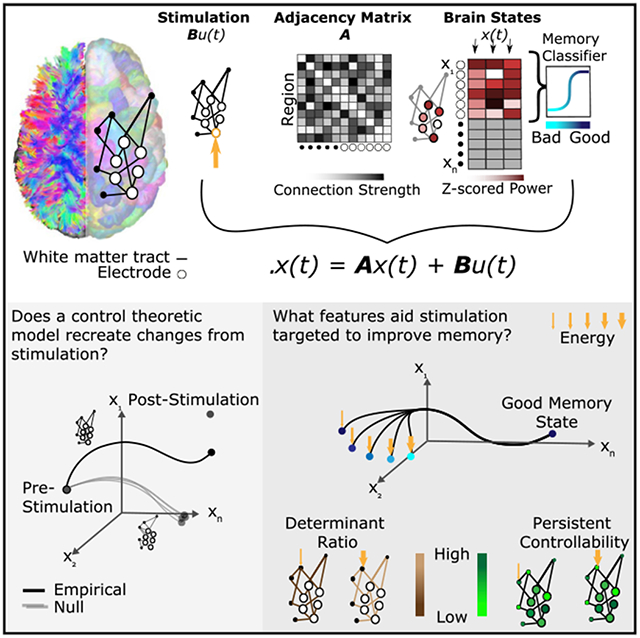
Optimizing direct electrical stimulation for the treatment of neurological disease remains difficult due to an incomplete understanding of its physical propagation through brain tissue. Here, we use network control theory to predict how stimulation spreads through white matter to influence spatially distributed dynamics. We test the theory’s predictions using a unique dataset comprising diffusion weighted imaging and electrocorticography in epilepsy patients undergoing grid stimulation. We find statistically significant shared variance between the predicted activity state transitions and the observed activity state transitions. We then use an optimal control framework to posit testable hypotheses regarding which brain states and structural properties will efficiently improve memory encoding when stimulated. Our work quantifies the role that white matter architecture plays in guiding the dynamics of direct electrical stimulation and offers empirical support for the utility of network control theory in explaining the brain’s response to stimulation.
Graphical Abstract
In Brief
Stiso et al. report evidence that network control theory can explain the propagation of electrical stimulation through the human brain and quantify how white matter connectivity is crucial for driving spatially distributed changes in activity. Furthermore, they use network control theory to predict stimulation outcome in specific cognitive contexts.
INTRODUCTION
Direct electrical stimulation has demonstrated clinical utility in detecting brain abnormalities during surgery (Li et al., 2011) and in mitigating symptoms of epilepsy, essential tremor, and dystonia (Sironi, 2011; Perlmutter and Mink, 2006; Lozano and Lipsman, 2013). Apart from clinical diagnosis and treatment, direct electrical stimulation has also been used to isolate the areas that are responsible for complex higher-order cognitive functions, including language (Jones et al., 2011; Mani et al., 2008), semantic memory (Shimotake et al., 2015), and face perception (Parvizi et al., 2012). An open and important question is whether such stimulation can be used to reliably enhance cognitive function, and if so, whether stimulation parameters (e.g., intensity, location) can be optimized and personalized based on individual brain anatomy and physiology. While some studies demonstrate enhancements in spatial learning (Lee et al., 2017) and memory (Ezzyat et al., 2018; Laxton et al., 2010; Ezzyat et al, 2017; Kucewicz et al., 2018; Suthana et al., 2012) following direct electrical stimulation, others show decrements (Jacobs et al., 2016; Kim et al., 2018b) (for a review, see Kim et al., 2016). Such conflicting evidence is also present in the literature on other types of stimulation, including transcranial magnetic stimulation. Proposed explanations range from variations in stimulation intensity (Reichenbach et al., 2011) to individual differences in brain connectivity (Downar et al., 2014).
A key challenge in circumscribing the utility of stimulation for cognitive enhancement or clinical intervention is the fact that we do not have a fundamental understanding of how an arbitrary stimulation paradigm applied to one brain area alters the distributed neural activity in neighboring and distant brain areas (Johnson et al., 2013; Laxton et al., 2010; Lozano and Lipsman, 2013). Models of stimulation propagation through brain tissue range in complexity and biophysical realism (McIntyre et al., 2004b) from those that only model the region being targeted to those that use finite element models to expand predictions throughout different tissue types (Yousif and Liu, 2009), including both gray matter and white matter (Kim et al., 2011). Even in the simpler simulations of the effects of stimulation on a local cell population, there are challenges in accounting for the orientation of cells and the distance from the axon hillock, which can lead to strikingly different circuit behaviors (McIntyre et al., 2004b). In the more expansive studies of the effects of stimulation across the brain, it has been noted empirically that minute differences in electrode location can generate substantial differences in which white matter pathways are directly activated (Lujan et al., 2013; Riva-Posse et al., 2014) and that the white matter connectivity of an individual can predict the behavioral effects of stimulation (Horn et al., 2017; Ellmore et al., 2009). These differences are particularly important in predicting the response to therapy, given recent observations that stimulation to white matter may be particularly efficacious in treating depression (Riva-Posse et al., 2013) and epilepsy (Toprani and Durand, 2013). Despite these critical observations, a first-principles intuition regarding how the effects of stimulation may depend on the pattern of white matter connectivity present in a single human brain has remained elusive.
Network control theory provides a potentially powerful approach for modeling direct electrical stimulation in humans (Tang and Bassett, 2017). Building on recent advances in physics and engineering, network control theory characterizes a complex system as composed of nodes interconnected by edges (Newman, 2010), and then specifies a model of network dynamics to determine how external input affects the time-varying activity of the nodes (Liu et al., 2011). Drawing on canonical results from linear systems and structural controllability (Kailath, 1980), this approach was originally developed in the context of technological, mechanical, and other man-made systems (Pasqualetti et al., 2014), but has notable relevance for the study of natural processes from cell signaling (Cornelius et al., 2013) to gene regulation (Zañudo et al., 2017). In applying such a theory to the human brain, one first represents the brain as a network of nodes (brain regions) interconnected by structural edges (white matter tracts) (Bassett and Sporns, 2017), and then one posits a model of system dynamics that specifies how control input affects neural dynamics via propagation along the tracts (Gu et al., 2015). Formal approaches built on this model address questions of where control points are positioned in the system (Gu et al., 2015; Tang et al., 2017; Muldoon et al., 2016; Wu-Yan et al., 2018), as well as how to define spatiotemporal patterns of control input to move the system along a trajectory from an initial state to a desired final state (Gu et al., 2017; Betzel et al., 2016). Intuitively, these approaches may be particularly useful in probing the effects of stimulation (Muldoon et al., 2016) and pharmacogenetic activation or inactivation (Grayson et al., 2016) for the purposes of guiding transitions between cognitive states or treating abnormalities of brain network dynamics such as epilepsy (Ching et al., 2012; Ehrens et al., 2015; Taylor et al., 2015), psychosis (Braun et al., 2018), or bipolar disorder (Jeganathan et al., 2018). However, this intuition has not yet been validated with direct electrical stimulation data.
Here, we posit a simple theory of brain network control, and we test its biological validity and utility in combined electrocorticography (ECoG) and diffusion weighted imaging (DWI) data from patients with medically refractory epilepsy undergoing evaluation for resective surgery. For each subject, we constructed a structural brain network in which nodes represented regions of the Lausanne atlas (Cammoun et al., 2012) and edges represented quantitative anisotropy between these regions estimated from diffusion tractography (Yeh et al., 2013) (Figure 1A). Upon this network, we stipulated a noise-free, linear, continuoustime, and time-invariant model of network dynamics (Gu et al., 2015; Betzel et al., 2016; Tang et al., 2017; Gu et al., 2017; Kim et al., 2018a) from which we built predictions about how regional activity would deviate from its initial state in the presence of exogenous control input to any given node. Using ECoG data acquired from the same individuals during an extensive direct electrical stimulation regimen (Figure 1B), we test these theoretical predictions by representing (1) regional activity as the power of an electrode in a given frequency band, (2) the pre-stimulation brain state as the power before stimulation, and (3) the poststimulation brain state as the power after stimulation (Figure 1C). After quantifying the relative accuracy of our theoretical predictions, we next use the model to make more specific predictions about the control energy required to optimally guide the brain from a pre-stimulation state to a specific target state. Here, we select a target state associated with successful memory encoding, although the model could be applied to any desired target. We quantify successful encoding states using subject-level power-based biomarkers of good memory encoding extracted with a multivariate classifier from ECoG data collected during a verbal memory task (Ezzyat et al., 2017). Finally, we investigate how certain topological (Kim et al., 2018a) and spatial (Roberts et al., 2016) properties of the network of a subject alter its response to direct electrical stimulation, and we ask whether that response is also modulated by control properties of the area being stimulated (Gu et al., 2015; Muldoon et al., 2016). Essentially, our study posits and empirically tests a simple theory of brain network control, demonstrating its utility in predicting response to direct electrical stimulation.
Figure 1. Schematic of Methods.
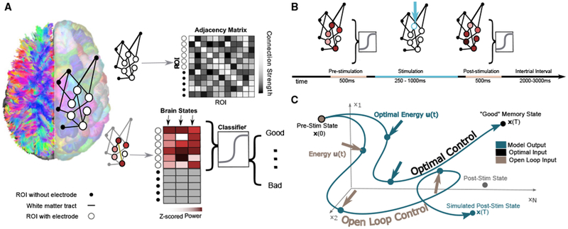
(A) Depiction of network construction and definition of brain state. (Left) We segment subjects’ diffusion weighted imaging data into N = 234 regions of interest using a Lausanne atlas (Cammoun et al., 2012). We treat each region as a node in a whole-brain network, irrespective of whether the region contains an electrode. Edges between nodes represent mean quantitative anisotropy (Yeh et al., 2013) along the streamlines connecting them. (Right, top) We summarize the network in an N×N adjacency matrix. (Right, bottom) A brain state is defined as the N×1 vector comprising activity across the N regions. Any element of the vector corresponding to a region with an electrode is defined as the band-limited power of ECoG activity measured by that electrode. Each brain state is also associated with an estimated probability of being in a good memory state, using a previously validated machine learning classifier approach (Ezzyat et al., 2017).
(B) Schematic of a single stimulation trial. First, ECoG data are collected for 500 ms. Then, stimulation is applied to a given electrode for 250–1,000 ms. Finally, ECoG data are again collected after the stimulation.
(C) Schematic of the open loop and optimal control paradigms. In the open loop design, energy u(t) is applied in silico at the stimulation site to the initial, prestimulation brain state x(0). The system will travel to some other state x(T), as stipulated by our model of neural dynamics, and we will measure the similarity between that predicted state and the empirically observed post-stimulation state. In the optimal control design, the initial brain state x(0) has some position in space that evolves over time toward a predefined target state x(T). At every time point, we calculate the optimal energy (u(t)) required at the stimulating electrode to propel the system to the target state.
RESULTS
Our model assumes the time-invariant network dynamics
| (Equation 1) |
where the time-dependent state x is an N×1 vector (N = 234) whose ith element gives the band-specific ECoG power in sensor i if i contained an electrode (xi = 1 otherwise); A is the N×N adjacency matrix estimated from DWI data; and B is an N×N matrix that selects the control set κ = u1,…,up, where p is the number of regions that receive exogenous control input (in most cases, p = 1). In our data, the stimulation site was typically the temporal lobe or cingulate (see Figure S1; Table S1 for further details regarding electrode location). The input is constant in time and given by u(t) = β × I × log(ω) × (Δt), where I is the empirical stimulation amplitude in amperes (range, 0.5–3 mA), ω is the empirical stimulation frequency in hertz (range, 10–200 Hz), and Δt is the number of simulated samples (here, 950) divided by the empirical stimulation duration (range, 250–1,000 ms) in seconds. Note that since our model is in arbitrary time units with no clear mapping onto physical units of time (i.e., seconds), we incorporate the duration of stimulation into the energy term — following the intuition that longer stimulation sessions add more total energy—rather than incorporating it into the number of time units. The free parameter β scales the input to match the units of x. Biologically, β reflects the relation between activity in a cell population and the current from an electrode, which in turn can be influenced by the orientation of the cells, the proximity of the cell body or axons to the electrode, and the quality of the electrode (McIntyre et al., 2004a) (see STAR Methods). This model formalizes the hypothesis that white matter tracts constrain how stimulation affects brain state and that those effects can be quantified using network control theory.
Predicting Post-stimulation States by Open Loop Control
We begin by exercising the model to determine whether our theory accurately predicts changes in brain state induced by direct electrical stimulation. Specifically, we simulate Equation 1 to predict how stimulation alone (independent of other ongoing intrinsic dynamics) will alter brain state, given the structural adjacency matrix A and the initial state x(0) comprising the ECoG power at every node recorded pre-stimulation (xi = 1 if node i is a region without electrodes and the Z scored power otherwise; see Figure S3 for further details). For each stimulation event, we calculate the Pearson’s correlation coefficient between the empirically observed post-stimulation state of regions of interest (ROIs) with electrode coverage (an electrode by frequency matrix) and the predicted post-stimulation state at every time point in the simulated trajectory x(t). Furthermore, xi = 1 if node i is a region without electrodes, and the Z scored power otherwise (including stimulating and non-stimulating electrodes). To measure the capacity of the model simulation to predict the poststimulation state, we measure the maximum correlation achieved across the model simulation time of a.u. Since there is no clear mapping of stimulated time steps onto physical units of time (i.e., seconds), we chose a number of time steps that were sufficient to allow correlation values to stabilize (Figure S1). In Figure S1, we provide evidence that results are highly consistent across different time step sizes as long as this stability has been reached. Accordingly, we compute a maximum correlation value across simulated time points between the model prediction and the empirically observed post-stimulation state for each stimulation trial (mean = 0.036, SD = 0.019; Figure 2A). We observe that the mean of the maximum correlation values is significantly greater than zero (t test N = 11, t = 5.83, p = 3.31 × 10⁻⁵). We note that this correlation represents the impact of stimulation alone on linear dynamics and does not take into account any other incoming stimuli from the surrounding environment or any ongoing cognitive or metabolic processes, nonlinear dependencies, or inter-frequency interactions (Canolty and Knight, 2010; Buzsáki et al., 2012; Peterson and Voytek, 2017). Complementing this estimate, we were also interested in the time point (measured in a.u.) at which the trial reached its largest magnitude correlation (positive or negative) before decaying toward zero. In our model, the white matter networks define the dynamics of how brain states evolve in time. In addition to affecting the amount that each region changes its activity, the pattern of connections also affects the dynamics of brain states, and how quickly input to the system will dissipate. If more time points are required (and the peak time is large), then energy needs longer to spread, and it needs to spread across higher-order connections compared to when the peak time is small. We observed that the time at which the peak magnitude occurred differed across trials, having a mean of 298 a.u. with an SD of 114 a.u. (Figure 2B).
Figure 2. Post-stimulation Brain State Depends on White Matter Network Architecture.
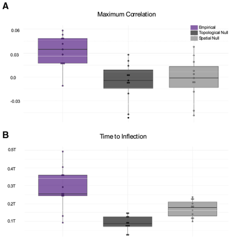
(A) Boxplots depicting the average maximum correlation between the empirically observed post-stimulation state and the predicted post-stimulation state at everytime point in the simulated trajectory x(t) for N = 11 subjects. Boxplots indicatethe median (solid horizontal black line) and quartiles ofthe data. Each data point represents a single subject, averaged over all of the trials (with different stimulation parameters).
(B) Boxplots depicting the average time to reach the peak magnitude (positive or negative) correlation between the empirically observed post-stimulation state and the theoretically predicted post-stimulation state at every time point in the simulated trajectory x(t). Time is measured in a.u. Color indicates theoretical predictions from Equation 1, where A is (1) the empirical network (purple) estimated from the diffusion imaging data, (2) the topological null network (dark charcoal), and (3) the spatial null network (light charcoal).
See also Figures S1 and S2.
To determine the influence of network geometry on our model predictions, we compared the empirical observations to those obtained by replacing A in the simulation with one of two null model networks, each designed to independently remove specific geometric features of the structural network (see Figure S5 for examples). First, for each trial, we constructed a topological null, a randomly rewired network that preserved the edge distribution, degree distribution, number of nodes, and number of edges. Second, we constructed a spatial null, a randomly rewired network that preserved the edge distribution, and the relation between edge strength and Euclidean distance. If the observed correlations are due to unique features of human white matter tracts (and not the number edges and their strength or patterns of connectivity that arise from the spatial embedding of the brain), then we would expect smaller correlations from the null models. Similarly, if the observed peak correlation times are due to the need for energy to spread to unique higher-order connections in human white matter networks, we would expect earlier peak times in the null models. Using a repeated-measures ANOVA, we find a significant main effect across null models (F(2,20) = 20.6, p = 1.37 × 10⁵), and the time at which the maximum correlation values occur (F(2,20) = 21.78, p = 9.50 × 10⁻⁶). We then performed post hoc analyses and found that the topological null produced significantly weaker maximum correlations between the empirically observed post-stimulation state and the simulated states (paired t test: N = 11, t = 4.82, uncorrected p = 7.04 × 10⁻⁴), which also peaked significantly earlier in time than the true data (N = 11, t = 6.68, uncorrected p = 5.47 × 10⁻⁵). The spatial null model also produced significantly weaker maximum correlations between the empirically observed post-stimulation state and the predicted post-stimulation states (permutation test N = 11, t = 4.27, uncorrected p = 1.65 × 10⁻³), which also occurred significantly earlier in time than that observed in the true data (N = 11, t = 2.83, uncorrected p = 0.018). We observed consistent results in individual subjects (after correcting for multiple comparisons, and with medium to large effect sizes) (Figure S2), across all of the frequency bands (Figure S2), with different values of β (Figure S1), and when using a smaller resolution atlas (Figure S2) for whole-brain parcellation. The only exception was that the spatial null models did not peak significantly earlier than the empirical models after Bonferroni correction for individual frequency bands (Figure S2). Considering individual variability in DWI estimates, we next asked whether our model would more accurately predict transitions with an individual’s own connectivity, compared to the connectivity of another subject in the same cohort. We did not find a significant difference (paired t test N = 11, t = −0.40, p = 0.70), indicating that our model generalizes across the subjects in this cohort and does not either depend or capitalize upon individual differences in connectivity. Overall, these observations support the notion that structural connections facilitate a rich repertoire of system dynamics following cortical stimulation and directly constrain the dynamic propagation of stimulation energy in the human brain in a manner that is consistent with a simple linear model of network dynamics.
Simulating State Transitions by Optimal Network Control
We next sought to use the model to better understand the principles constraining brain state transitions in the service of cognitive function and their response to exogenous perturbations in the form of direct electrical stimulation. Building on the network dynamics stipulated in Equation 1, we used an optimal control framework to calculate the optimal amount of external input u to deliver to the control set K containing the stimulating electrode, driving the system from a specific pre-stimulation state toward a target post-stimulation state (Figure 1C). Put differently, rather than predicting the brain state changes associated with empirical stimulation for input as we did with our open-loop control model, the optimal control model will analytically solve for the optimal input to get to a specific state. Because this model will necessarily reach the target state that is specified, the optimal control model is better suited to make theoretical predictions about where and when to stimulate rather than to predict state changes based on a certain stimulation paradigm. Here, the specific (or target) post-stimulation state was defined as a period with a high probability of successfully encoding a memory and was operationalized using a previously validated classifier constructed from ECoG data from the same subjects during the performance of a verbal memory task (Ezzyat et al., 2017) (Figure 1A). We use this target state as a simple, data-driven estimate of a single behaviorally relevant state for illustrative purposes rather than as an exhaustive account of successful memory processes. To determine the optimal input, we use a cost function that minimizes both the energy and the difference of the current state from the target state:
| (Equation 2) |
where xT is the target state, S is a diagonal N×N matrix that selects a subset of states to constrain (here, S is the identity and all diagonal entries are equal to 1), ρ is the importance of the input penalty relative to the state penalty, T is the time allotted for the simulation, and the prime indicates a matrix transposition (see Figure S3 and STAR Methods for details about parameter selection). Since the input u(t) is being solved for rather than defined by the user, we do not differentiate between the different stimulation parameters used in different trials. We note that optimizing the cost function in Equation 2 necessarily identifies simulated optimal control trajectories from the pre-stimulation state to a good memory state reasonably close to the target (final distance from target mean = 0.12, SD = 0.06) with minimal error (range from 3.65×10⁻⁵ to 5.19 × 10⁻⁴).
We begin by addressing the hypothesis that greater energy should be required to reach the target state when it is farther from the initial state. We operationalize this notion by defining distance in four different ways. We define distance as the Frobenius norm of the difference between initial and target states. We fit a linear mixed effects model to the integral of the input squared, or energy (here, Bu) in every trial, treating the Frobenius norm distance between initial and final state as a fixed effect, and treating subject as a random effect. We find that the distance between the initial and the final state is positively related to the energy required for the transition (β = 8.3 × 10⁻³, t(7,547) = 18.11, p < 2 × 10⁻¹⁶) (Figure 3A). Although this result is fairly intuitive, it is also important to consider other measurements of distance that are more informed by biological intuitions about the energy landscape of the brain. Second, we define distance by the memory capacity in the initial state. It is important to keep in mind that this memory state is defined by a previously trained and validated classifier and not by task performance during stimulation. We fit a linear mixed effects model to the integral of the input squared in every trial, treating the probability of the initial state of successfully encoding a memory as a fixed effect and treating subject as a random effect. We find that the probability of the initial state of successfully encoding a memory is negatively related to the energy required for the transition (β = −0.18, t(7,547) = 14.4, p < 2 × 10⁻¹⁶). We also find that the probability of the initial state of successfully encoding a memory explains variance in the energy required for the transition independent of the Frobenius norm distance (linear mixed effects model including both distance measures: initial probability t(7,547) = −7.09, p = 1.47 × 10⁻¹²; Frobenius norm t(7,547) = 12.98, p < 2 × 10⁻¹⁶) (Figure 3B). These findings suggest that states that begin closer to the target require less energy to reach the target. Third, we define distance as the observed change in memory state resulting from stimulation. We fit a linear mixed effects model to the input squared in every trial, treating the change in memory state as a fixed effect and treating subject as a random effect. We find that the change in memory state is positively related to the energy required for the transition (β = 9.5 × 10⁻², t(7,547) = 8.43, p < 2 × 10⁻¹⁶) (Figure 3C). These results were consistent across two alternate sets of optimal control parameters (Figure S4).
Figure 3. Longer-Distance Trajectories Require More Stimulation Energy.
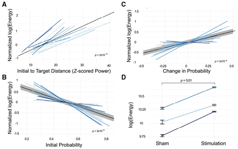
(A) The normalized energy required to transition between the initial state and the post-stimulation state, as a function of the Frobenius norm between the initial state and the post-stimulation state. The black solid line represents the best linear fit (with gray representing standard error) and is provided simply as a guide to the eye (β = 8.3 × 10⁻³, t = 18.11, p < 2 × 10⁻¹⁶). Normalization is also performed to enhance visual clarity.
(B) The energy required to transition to a good memory state, as a function of the initial probability of being in a good memory state (β = −0.18, t = −14.4, p < 2 × 10⁻¹⁶).
(C) The energy required to transition to a good memory state as a function of the empirical change in memory state resulting from stimulation (β = 9.5 × 10⁻², t = 8.43, p < 2 × 10⁻¹⁶).
(D) In N = 3 experimental sessions that included both sham and stimulation trials, we calculated the energy required to reach the post-stimulation state or the post-sham state, rather than a target good memory state. Here, we show the difference in energy required for sham state transitions in comparison to stimulation state transitions (paired t test, N = 3, p = 0.01). Error bars indicate SEMs across trials. Across all four panels, different shades of blue indicate different experimental sessions and subjects (N = 16).
See also Figure S4.
This set of results serves as a basic validation that transitions between nearby brain states will generally require less energy than transitions between distant states. This finding holds whether distance is defined in terms of the difference in Frobenius norm between matrices of regional power or in terms of the estimated probability to support the cognitive process of memory encoding. In specificity analyses, we also determined whether these relations were expected in appropriate random network null models. We observed that the relations were significantly attenuated in theoretical predictions from Equation 1, where A is either the topological null network (N = 7,547, p = 6.1 × 10⁻⁴) or the spatial null network (N = 7,547, p = 0.0017) (Figure S4). We also found that the largest differences between the empirical relations and those expected in the null networks were observed in the context of biological measures of distance (e.g., initial probability, change in probability), with only modest differences seen in the statistical measure of distance (the Frobenius norm).
As a fourth and final test of the biological relevance of these findings, we considered sham trials, in which no stimulation was delivered, as compared to stimulation trials. We expect that the state that the brain reaches after stimulation is farther away from the initial state than the state that the brain reaches naturally at the conclusion of a sham trial. We first examine this expectation in the context of the Frobenius norm distance discussed above. We observed that two out of the three experimental sessions that included sham stimulation displayed significantly larger distances (measured by the Frobenius norm) between pre-and post-stimulation states for stimulation conditions than for sham conditions (permutation test, N > 192, p < 6.8 × 10⁻³ for all subjects). We next tested whether more energy would be required to simulate the transition from the initial pre-stimulation state to the post-stimulation state than from the initial pre-sham state to the post-sham state. We found consistently greater energy for stimulation trials compared to sham trials in all of the datasets (paired t test, N = 3, p = 0.01; Figure 3D). We further confirmed this finding with a non-parametric permutation test assessing differences in the distribution of energy values across trials for sham conditions and the distribution of energy values across trials for stimulation conditions (permutation test, N > 192, p < 2 × 10⁻¹⁶ for all subjects). These observations support the notion that transitions between nearby brain states occur without stimulation (sham) and require little predicted energy, whereas transitions between distant brain states occur with stimulation and require greater predicted energy.
The Role of Network Topology in Stimulation-Based Control
While it is natural to posit that the distance between brain states is an important constraint on the ease of a state transition, there are other important principles that are also likely to play a critical role. Paramount among them is the architecture of the network available for the transmission of control signals. We therefore turn to the question of which features of the network predict the amount of energy required for each transition from the prestimulation state to a good memory state. To address this question, we considered the empirical networks as well as the topological and spatial null model networks discussed earlier. We find that the optimal control input energy required for these state transitions differs across network types (one-way repeated-measures ANOVA F(2,20) = 14.75, p = 1.06 × 10⁻⁴). In post hoc testing, we found that the optimal control energy was significantly different between the empirical network and the topological null network (paired t test: N = 11, t = 3.64, p = 4.6 × 10⁻³) (Figure 4A), but not between the empirical network and the spatial null network (N = 11, t = − 1.80, p = 0.10). This observation suggests that the spatial embedding that characterizes both the real network and the spatial null network may increase the difficulty of control. In supplemental analyses (Figure S5), we test two additional spatially embedded null models that further preserve degree distribution and strength sequence, and we find similar average energies to the empirical and spatial null models discussed here (see Figure S5). We hypothesized that the difference in optimal control energy could be mechanistically explained by the determinant ratio, a recently proposed metric quantifying the trade-off between connection strength (facilitating control) and connection homogeneity (hampering control) (Kim et al., 2018a). A network with a high determinant ratio will have weak, homogeneous connections between the control nodes and nodes being controlled. We found that across all of the networks, the determinant ratio explains a significant amount of variance in energy after accounting for network type (linear mixed effects model with network type and determinant ratio as fixed effects: χ2(2, N = 33) = 13.3, p = 2.65 × 10⁻⁵) (Figure 4B). These results support the notion that spatial embedding could impose energy barriers by compromising the trade-off between the strength and homogeneity of connections emanating from the stimulating electrode (see Figure S5 for extensions to other spatially embedded null models).
Figure 4. Topological and Spatial Constraints on the Energy Required for Stimulation-Based Control.
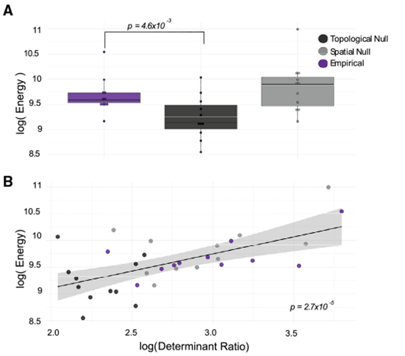
(A) Average input energy required for each transition from the pre-stimulation state to a good memory state, as theoretically predicted from Equation 1, where A is (1) the empirical network (purple) estimated from the diffusion imaging data, (2) the topological null network (dark charcoal), and (3) the spatial null network (light charcoal) for N = 11 subjects.
(B) The relation between the determinant ratio and the energy required for the transition from the pre-stimulation state to a good memory state. The color scheme is identical to that used in (A). The p value is from a paired t test: N = 11, t = 3.64, p = 4.6 × 10⁻³.
See also Figure S5.
Characteristics of Efficient Regional Controllers
Thus far, we have seen that the distance of the state transition and the architecture of the network available for the transmission of control signals both affect the energy required. However, neither of these factors address the potential importance of anatomical characteristics specific to the region being stimulated. Such regional effects are salient in the 1 subject (S8, 3 stimulation sessions across 7 unique electrodes) in our patient sample who had multiple empirical stimulation sites spanning the same number of ROIs. Since both sites span the same number of ROIs, we know that any differences in energy cannot be due to differences in the size of the control set used in the stimulation. In this patient, we found that transitions from the observed initial state to a good memory state required significantly greater energy when stimulation was delivered to electrodes in the middle temporal region than when stimulation was delivered to the inferior temporal region (permutation test, N = 555, p < 2 × 10⁻¹⁶) (Figure 5A). We hypothesized that this sensitivity to anatomical location could be mechanistically explained by regional persistent and transient modal controllability, which quantify the degree to which specific eigenmodes of the dynamics of the network can be influenced by input applied to that region (Figure S6). Energetic input to nodes with high persistent controllability will result in large perturbations to slowly decaying modes of the system, while energetic input to nodes with high transient controllability will result in large perturbations to quickly decaying modes of the system.
Figure 5. Role of Local Topology Around the Region Being Stimulated.
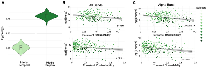
(A) Transitions from the observed initial state to a good memory state required significantly greater energy when affected by the middle temporal sensors than when affected by the inferior temporal sensors.
(B) Relation between persistent (χ2 = 3.89, p = 0.049) (top) or transient (χ2 = 1.69, p = 0.19) (bottom) controllability of the stimulated region and the energy predicted from optimal transitions from the initial state to a good memory state. We only allow energy to be injected into a single electrode-containing region, and we consider a broadband state matrix.
Every color is a subject (N = 11) and every dot is a different simulated stimulation site.
(C) As in (B), but when considering the α band state vector only (persistent controllability: χ2 = 13.8, p = 2.00 × 10⁻⁴; transient controllability: χ2 = 11.4, p = 7.5 × 10⁻⁴).
See also Figure S6.
To test our hypothesis, we simulated optimal trajectories from the initial state to a good memory state while only allowing energy to be injected into a single electrode-containing region (irrespective of whether empirical stimulation was applied there). We then compared the energy predicted from these simulations to the regional controllability. We found a significant relation between persistent (but not transient) modal controllability of the region being stimulated and the input energy of the state transition (linear mixed effects model accounting for subject: persistent controllability χ2(1,374) = 3.89, p = 0.049, transient controllability χ2(1,374) = 1.69, p = 0.19) (Figure 5B). We note that the strength of the region being stimulated was not a significant predictor of energy (linear mixed effects model χ2(1,374) = 3.5, p = 0.061), although there is only a small difference between the predictive power of strength and persistent controllability. In addition, in the one subject who had two empirical stimulation locations, we observed that the middle temporal stimulation site with larger energy requirements had smaller persistent controllability (0.058) than the inferior temporal site with smaller energy (0.072). Given this modest effect for broadband state transitions, we next asked whether the influence of regional controllability varied based on the specific frequency band being controlled. Notably, we found that both transient and persistent controllability showed strong relations to energy in the α band (linear mixed effects model: persistent controllability χ2(1,374) = 13.8, p = 2.00 × 10⁻⁴, transient controllability χ2(1,374) = 11.4, p = 7.5 × 10⁻⁴; Bonferroni corrected for multiple comparisons across frequency bands) (Figure 5C). Persistent controllability alone also showed a statistically significant relation for the high γ band (linear mixed effects model: persistent controllability χ2(1,374) = 12.2,p = 4.67 × 10⁻⁴)(Figure S6). These findings suggest that the local white matter architecture of the stimulated regions can support the selective control of slowly damping dynamics.
Effective Prediction of Energy Requirements
In the previous section, we presented a series of analyses with the goal of elucidating what aspects of brain state and white matter connectivity affect the energy requirements predicted by our model in an effort to better understand the network-wide effects of direct electrical stimulation. Here, we conclude by synthesizing these results into a single model to predict the energy requirements of a stimulation paradigm, given the persistent controllability of the region to be stimulated, the determinant ratio of the network to be controlled, and the probability of encoding a memory at the time of stimulation (Figure 6A). We fit a random forest model to predict energy given these inputs from our data, and we compared the performance of this model to the performance of a distribution of 1,000 models in which the association between energy values and predictors was permuted uniformly at random. We found that our model had an out-of-bag mean squared error of 9.28 × 10⁻³, which was substantially lower than the null distribution (mean = 9.62×10⁻³ and SD = 2.97 × 10⁻⁵). We also found that our model explained 93.2% of the variance in the predicted energy of the state transition. Random forest models also produce a measure of variable importance, which represents the degree to which including these variables tends to reduce the prediction error. We found that the determinant ratio was the most important (increased node purity = 627), followed by the persistent controllability (320), followed by the initial probability of encoding a memory (23.0). Broadly, these results suggest that the energy requirements for a specific state transition can be accurately predicted given the simple features of the connectome and the current brain state.
Figure 6. Network Topology and Brain State Predict Energy Requirements.
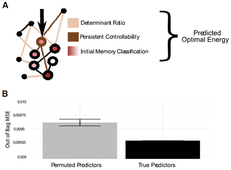
(A) Schematic of the three topology and state features included in the random forest model that we built to predict energy requirements. Network-level effects (tan) are captured by the determinant ratio, regional effects (brown) are captured by persistent controllability, and state-dependent effects (red) are captured by the initial memory state.
(B) Comparison of the out-of-bag mean squared error for a model in which each subject’s (N = 11) determinant ratio, persistent controllability, and initial memory state are used to predict their required energy. We compared the performance of this model to the performance of a distribution of N = 1,000 models in which the association between energy values and predictors was permuted uniformly at random.
DISCUSSION
While direct electrical stimulation has great therapeutic potential, its optimization and personalization remain challenging, in part due to a lack of understanding of how focal stimulation affects the state of both neighboring and distant regions. Here, we use network control theory to test the hypothesis that the effect of direct electrical stimulation on brain dynamics is constrained by the white matter connectivity of an individual. By stipulating a simplified noise-free, linear, continuous-time, and time-invariant model of neural dynamics, we demonstrate that time-varying changes in the pattern of ECoG power across brain regions is better predicted by the true white matter connectivity of an individual than either topological or spatial network null models. We build on this observation by positing a model for exact brain state transitions in which the energy required for the state transition is minimized, as is the length of the trajectory through the available state space. We use this model to make theoretical predictions about how white matter architecture and brain states make stimulation to these specific states easier. We demonstrate that transitions between more distant states are predicted to require greater energy than transitions between nearby states; these results are particularly salient when distance is defined based on differences in the probability with which a cross-regional pattern of ECoG power supports memory encoding. In addition to the distance between initial and target states, we find that regional and global characteristics of the network topology predict the energy required for the state transition: networks with smaller determinant ratios (stronger, less homogeneous connections) and stimulation regions with higher persistent controllability tend to demand less energy. Finally, we demonstrate that these two topological features in combination with the initial brain state explain 93% of the variance in required energy across subjects. Overall, our study supports the notion that control theoretic models of brain network dynamics provide biologically grounded, individualized hypotheses of response to direct electrical stimulation by accounting for how white matter connections constrain state transitions.
A Role for Network Control Theory in Modern Neuroscience
Developing theories, models, and methods for the control of neural systems is not a new goal in neuroscience. Whether in support of basic science (e.g., seminal experiments from Hodgkin and Huxley) or in support of clinical therapies (e.g., technological development in brain-machine interfaces or deep brain stimulation), efforts to control neural activity have produced a plethora of experimental tools with varying levels of complexity (Schiff, 2011). Building on these empirical advances, the development of a theory for the control of distributed circuits is a logical next step. Network control theory is one particularly promising option. In assimilating brain state and connectivity in a mathematical model (Schiff, 2011), network control theory offers a first-principles approach to modeling neural dynamics, predicting its response to perturbations, and optimizing those perturbations to produce a desired outcome. In cellular neuroscience, network control theory has offered predictions of the functional role of individual neurons in Caenorhabditis elegans, and those predictions have been validated by perturbative experiments (Yan et al., 2017). While the theory has also offered predictions in humans (Gu et al., 2015; Muldoon et al., 2016; Ching et al., 2012; Taylor et al., 2015; Jeganathan et al., 2018), these predictions have not been validated in accompanying perturbative experiments. Here, we address this gap by examining the utility of network control theory in predicting empirically recorded brain states and by validating the fundamental assumption that state transitions are constrained by the white matter connectivity of an individual. The work provides theoretical support for emerging empirical observations that structural connectivity can predict the behavioral effects of stimulation (Horn et al., 2017; Ellmore et al., 2009), thus constituting an important first step in establishing the promise and utility of control theoretic models of brain stimulation.
The Principle of Optimal Control in Brain State Transitions
By positing a model for optimal brain state transitions, we relate expected energy expenditures to a simple, validated estimate of memory encoding, directly relating the theory to a desired behavioral feature. This portion of the investigation was made possible by an important modeling advance addressing the challenge of simulating a trajectory whose control is dominated by a single node—the stimulating electrode. This type of control is an intuitive way to model stimulation, in which one wishes to capture changes resulting from a single input source. However, prior work has demonstrated that while the brain is theoretically controllable from a single point, the amount of energy required can be so large as to make the control strategy impractical (Gu et al. (2015). Here, we extend prior models of optimal control (Betzel et al., 2016; Gu et al., 2017) by relaxing the input matrix B such that it allows large input to stimulated regions, but also allows small, randomly generated amounts of input at other nodes in the network. This approach greatly lowers the error of the calculation and also produces narrowly distributed trajectories for the same inputs (see STAR Methods).
Topological Influencers of Control
Beyond the distance of the state transition, we found that both local and global features of the network topology were important predictors of control energy. In line with previous work investigating controllability radii (Menara et al., 2018), energy requirements were lower for randomly rewired networks. Both empirical and topological graphs share the common feature of modularity (Chen et al., 2013), which is destroyed in random topological null models (Roberts et al., 2016). Prior theoretical work has demonstrated that modularity is one way in which to decrease the energy of control by decreasing the determinant ratio, a quantification of the relation between the strength and heterogeneity of direct connections from the controlling node to others (Kim et al., 2018a). Here, we confirmed that the determinant ratio accurately predicted the required energy, while leaving a small amount of variance unexplained. We expected that this unexplained variance could be somewhat accounted for by features of the local network topology surrounding the stimulated node (Tang et al., 2017). Consistent with our expectation, we found that persistent controllability was the only significant predictor of energy across all frequency bands, indicating a specific role of slow modes in these state transitions. The effect was particularly salient in two bands with consistent (yet different) activity patterns in memory encoding—the α band and the high γ band (Fell et al., 2011; Buzsáki and Moser, 2013). Future avenues for research could include a comprehensive investigation of whether and why different regional topologies facilitate the control of frequency bands with distinct characteristic changes.
Clinical Implications
Our study represents a first step toward developing a control theoretic model to answer two pressing questions in optimizing direct electrical stimulation to meet clinical needs: (1) what changes in the brain after a specified stimulation event and (2) which regions are most effective to stimulate. Network control is by no means the only candidate model for answering these questions (McIntyre et al., 2004b; Yousif and Liu, 2009; Kim et al., 2011). Nevertheless, it is a particularly promising model in that it can account for global changes to focal events, is generalizable across any initial and target brain state, and is specific to each individual and his or her white matter architecture. The linear model of dynamics only captures a small amount of variance observed after stimulation, but stands to benefit from an expansion of the model to nonlinear models of dynamics, to time-varying changes in connectivity, and to field spread of stimulation. We also show that the optimal control energy for a given transition captures intuitions about the energy landscape of the brain despite being based on simplified linear dynamics. This metric was then used to identify features of white matter architecture that could facilitate control. Investigation into whether metrics could be incorporated into existing multimodal predictions of stimulation outcome is a logical next step in developing a tool for the clinical selection of stimulation regions. Finally, an evaluation of long-term efficacy of specific stimulation paradigms informed by principles of network control is warranted and would benefit from work in non-human animal models in which precise measurements of plasticity are accessible.
Methodological Considerations
Primary Data
As with any model of complex biological systems, our results must be interpreted in the context of the underlying data. First, we note that DWI data provide an incomplete picture of white matter organization, and even state-of-the-art tractography algorithms can identify spurious connections (Thomas et al., 2014). As higher resolution imaging, reconstruction, and tractography methods emerge, it will be important to replicate the results we report here. Second, while ECoG data provide high temporal resolution, it is collected from patients with epilepsy and results may not generalize to a healthy population (Parvizi and Kastner, 2018). However, it is worth noting that recent work has shown that tissue damage resulting from recurrent seizures can be minimal (Rossini et al., 2017), and most electrodes are not placed in epileptic tissue (Parvizi and Kastner, 2018). Nevertheless, this population can display atypical physiological signatures of memory (Glowinski, 1973), as well as atypical white matter connectivity (Gross et al., 2006). It will be important to extend this work to non-invasive techniques accessible to healthy individuals.
Modeling Assumptions
Our results must also be interpreted in light of model assumptions. First, we consider a relaxed input matrix to ensure that state transitions are primarily influenced by the set of stimulating electrodes and, to a lesser extent, non-stimulating electrodes. This choice is not a true representation of single-point control, but instead reflects the fact that the system is constantly modulated by endogenous sources (Gu et al., 2017; Betzel et al., 2016). Second, our model uses a time-invariant connectivity matrix. While DWI data are relatively stable over short timescales, repeated stimulation can result in dynamic changes in plasticity that are not captured here (Malenka and Bear, 2004).
Lastly, we note that our model assumes linear network dynamics. While the brain is not a linear system, such simplified approximations can predict features of fMRI data (Honey et al., 2007), predict the control response of nonlinear systems of coupled oscillators (Feldt Muldoon et al., 2013), and more generally provide enhanced interpretability over nonlinear models (Kim and Bassett, 2019). Nevertheless, considering control in nonlinear models of neural dynamics will constitute an important next step for two reasons. First, nonlinear models of brain dynamics can capture a richer repertoire of brain states that is more consistent with the repertoire observed in neural data (Jirsa et al., 2014; Jirsa and Haken, 1996; Breakspear et al., 2003; Messé et al., 2014, 2015; Hansen et al., 2015). Second, nonlinear approaches offer distinct types of control strategies. Specifically, linear control is frequently used to examine the transition between an initial state and a final state. Yet, some hypotheses about neural function may benefit from nonlinear control approaches such as feedback vertex set control (Zañudo et al., 2017; Cornelius et al., 2013) that allow one to examine the transition from one manifold of activity to another (Slotine and Li, 1991; Sontag, 2013). Such attractor-based control seems intuitively appropriate for the study of complex behaviors that are not well characterized by a single pattern of activity, but rather by a different trajectory through many states. Despite some progress, nonlinear approaches still lag far behind linear control approaches in their applicability and capability, and thus further theoretical work is needed (Slotine and Li, 1991; Sontag, 2013).
Defining Brain States
In our model, a brain state represents the Z scored power across electrodes in eight logarithmically spaced frequency bands from 1 to 200 Hz. This choice was guided by (1) the goal of maintaining consistency with the brain states on which the memory classifier was trained and (2) the fact that power spectra are well-documented behavioral analogs for memory (Ezzyat et al., 2017; Fell et al., 2011; Buzsáki and Moser, 2013). However, since many power calculations require convolution with a sine wave, power is insensitive to non-sinusoidal and phase-dependent features of the signal (Schalket al., 2017; Cole et al., 2017; Vinck et al., 2011). It would be interesting to explore transitions in other state spaces, such as instantaneous voltage (Schalk et al., 2017). Lastly, it is important to note that our algorithm controls each frequency band independently, although incorporating inter-frequency coupling (Peterson and Voytek, 2017; Bonnefond et al., 2017; Canolty and Knight, 2010) could be an interesting direction for future work. These considerations involving brain state also affect the interpretation of our target state as a good memory state. While our selection of target state does not exhaustively sample patterns of brain activity in which successful encoding can occur and only makes claims about a narrow range of all memory processes (encoding specifically), for the purposes of exploring the utility of network control theory in modeling direct stimulation, this classifier provides an important, if relatively narrow, behavioral link.
Conclusions and Future Directions
Our study begins to explore the role of white matter connectivity in guiding direct electrical stimulation, with the goal of driving brain dynamics toward states with a high probability of memory encoding. We demonstrate that our model of targeted direct electrical stimulation tracks well with biological intuitions and is influenced by both regional and global topological properties of underlying white matter connectivity. Overall, we show that our control theoretic model is a promising method that has the potential to inform hypotheses about the outcome of direct electrical stimulation.
STAR★METHODS
LEAD CONTACT AND MATERIALS AVAILABILITY
Raw data can be obtained upon request from http://memory.psych.upenn.edu/Request_RAM_Public_Data_access. This study did not generate any new data outside of the RAM project. Original code used in this project can be found at https://github.com/jastiso/NetworkControl. Further information and requests for resources should be directed to and will be fulfilled by the Lead Contact, Danielle Bassett (dsb@upenn.edu).
EXPERIMENTAL MODEL AND SUBJECT DETAILS
Subject Details
Electrocorticography and diffusion weighted imaging data were collected on eleven subjects (age 32 ± 10 years, 63.6% male and 36.4% female) as part of a multi-center project designed to assess the effects of electrical stimulation on memory-related brain function. Data were collected at Thomas Jefferson University Hospital and the Hospital of the University of Pennsylvania. The research protocol was approved by the institutional review board (IRB approval number 820553) at each hospital and informed consent was obtained from each participant.
Electrocorticography – ECoG
Electrophysiological data were collected from electrodes implanted subdurally on the cortical surface as well as deep within the brain parenchyma. In each case, the clinical team determined the placement of the electrodes to best localize epileptogenic regions. Subdural contacts were arranged in both strip and grid configurations with an inter-contact spacing of 10 mm. Depth electrodes had 8-12 contacts per electrode, with 3.5 mm spacing.
Electrodes were anatomically localized using separate processing pipelines for surface and depth electrodes. To localize depth electrodes we first labeled hippocampal subfields and medial temporal lobe cortices in a pre-implant, 2 mm thick, coronal T2-weighted MRI using the automatic segmentation of hippocampal subfields (ASHS) multi-atlas segmentation method (Yushkevich et al., 2015). We additionally used whole brain segmentation to localize depth electrodes not in medial temporal lobe cortices. We next co-registered a post-implant CT with the pre-implant MRI using Advanced Normalization Tools (ANTs) (Avants et al., 2008). Electrodes visible in the CT were then localized within subregions of the medial temporal lobe by a pair of neuroradiologists with expertise in medial temporal lobe anatomy. The neuroradiologists performed quality checks on the output of the ASHS/ANTs pipeline. To localize subdural electrodes, we first extracted the cortical surface from a pre-implant, volumetric, T1-weighted MRI using Freesurfer (Fischl et al., 2004). We next co-registered and localized subdural electrodes to cortical regions using an energy minimization algorithm. For patient imaging in which automatic localization failed, the neuroradiologists performed manual localization of the electrodes.
Intracranial data were recorded using one of the following clinical electroencephalogram (EEG) systems (depending on the site of data collection): Nihon Kohden EEG-1200, Natus XLTek EMU 128, or Grass Aura-LTM64. Depending on the amplifier and the preference of the clinical team, the signals were sampled at either 500 Hz, 1000 Hz or 1600 Hz and were referenced to a common contact placed either intracranially, on the scalp, or on the mastoid process. Intracranial electrophysiological data were filtered to attenuate line noise (5 Hz band-stop fourth order Butterworth, centered on 60 Hz). To eliminate potentially confounding large-scale artifacts and noise on the reference channel, we re-referenced the data using a bipolar montage. To do so, we identified all pairs of immediately adjacent contacts on every depth electrode, strip electrode, and grid electrode, and we took the difference between the signals recorded in each pair. The resulting bipolar timeseries was treated as a virtual electrode and used in all subsequent analysis. We performed spectral decomposition of the signal into 8 logarithmically spaced frequencies from 3 to 180 Hz. Power was estimated with a Morlet wavelet, in which the envelope of the wavelet was defined with a Gaussian kernel that allowed for 5 oscillations of the frequency of interest (one of 8, from 3-180 Hz). This kernel was then convolved with 500 ms epochs of ECoG data before and after stimulation to obtain estimates of power. The resulting time-frequency data were then log-transformed, and z-scored within session and within frequency band across events.
Diffusion Weighted Imaging – DWI
Diffusion imaging data were acquired from either the Hospital for the University of Pennsylvania (HUP), or Jefferson University Hospital. At HUP, all scans were acquired on a 3T Siemens TIM Trio scanner with a 32-channel phased-array head coil. Each data acquisition session included both a DWI scan as well as a high-resolution T1-weighted anatomical scan. The structural scan was conducted with an echo planar diffusion weighted technique acquired with iPAT using an acceleration factor of 2. The diffusion scan had a b value of 2000 s/mm2 and TE/TR = 117/4180 ms. The slice number was 92. Field of view read was 210 mm and slice thickness was 1.5 mm. Acquisition time per DWI scan was 8:26 min. The anatomical scan was a high-resolution 3D T1-weighted sagittal whole-brain image using an MPRAGE sequence. It was acquired with TR = 2400 ms; TE = 2.21 ms; flip angle = 8 degrees; 208 slices; 0.8 mm thickness. At Jefferson University Hospital, all scans were acquired on a 3T Philips Acheiva scanner. Each data acquisition session included both a DWI scan as well as a high-resolution T1-weighted anatomical scan. The diffusion scan was 61-directional with a b value of 3000 s/mm2 and TE/TR = 7517/98 ms, in addition to 1 b0 images. Matrix size was 96 × 96 with a slice number of 52. Field of view was 230 × 130 × 230 mm2 and slice thickness was 2.5 mm. Acquisition time per DWI scan was just over 9 min. The anatomical scan was a high-resolution 3D T1-weighted sagittal whole-brain image using an MPRAGE sequence. It was collected in sagittal orientation with in-plane resolution of 256 × 256 and 1 mm slice thickness (isotropic voxels of 1 mm3, 170 slices, TR = 650 ms, TE = 3.2 ms, Field of view 256 mm, flip angle 8 degrees, SENSE factor = 1, duration = 5 min).
Diffusion volumes were skull-stripped using FSL’s BET, v5.0.10. Volumes were subsequently corrected for eddy currents and motion using FSL’s EDDY tool, v.5.0.10 (Andersson and Sotiropoulos, 2016). Anatomical scans were processed with FreeSurfer v6.0.0. Surface reconstructions were used to generate subject-specific parcellations based on the Lausanne atlas from the Connectome Mapper Toolbox (Daducci et al., 2012). Each parcel was then individually warped into the subject’s native diffusion space. Using DSI-Studio, orientation density functions (ODFs) within each voxel were reconstructed from the corrected scans using GQI (Yeh et al., 2013). We then used the reconstructed ODFs to perform a whole-brain deterministic tractography using the derived QA values in DSI-Studio (Yeh et al., 2013). We generated 1,000,000 streamlines per subject, with a maximum turning angle of 35 degrees and a maximum length of 500 mm (Cieslak and Grafton, 2014). We hold the number of streamlines between participants constant (Griffa et al., 2013).
METHOD DETAILS
Stimulation Protocol
During each stimulation trial, we delivered stimulation using charge-balanced, biphasic, rectangular pulses with a pulse width of 300 μs. We cycled over the following parameters in consecutive trials: pulse frequency (10–200 Hz), pulse amplitude (0.5–3.0 mA), stimulation duration (0–1 s), and inter-stimulation interval (2.75–3.25 s). These stimulation parameter ranges were chosen to be well below the accepted safety limits for charge density, and ECoG was continuously monitored for after-discharges by a trained neurologist. Some subjects (N = 8) only received stimulation to one set of regions, while other received stimulation to multiple sets of regions (N = 3) (Table S1) Each subjects stimulating electrodes are shown in Figure S7. Most electrodes were in the temporal lobe, with some in the cingulate and frontal lobe.
Memory State Classification and Good Memory State Definition
Prior to collecting the data used in this study, each subject had a memory classifier trained based on their performance during a verbal memory task. The input data that we used was the spectral power averaged across the time dimension for each word encoding epoch (0–1600ms relative to word onset). Each subject’s personalized classifier was then used to return a likelihood of being in a good memory state for each pre- and post-stimulation recording. For more information about the classifier and the task design, see Ezzyat et al. (2017). A good memory state was defined for each subject using this classifier output. The target state was defined as the average of the top 5% of states with the largest probabilities (returned from the classifier) associated with them. The threshold of 5% was chosen as the smallest threshold that reliably included sufficient trials in the average (minimum number of trials was 192). The probabilities associated with these final target states ranged from 0.61 to 0.74.
The Mathematical Model - Open Loop Control
We use network control theory to model the effect of stimulation on brain dynamics because it accounts for systems level properties of brain states alongside external input. The theory requires us to stipulate a model of brain dynamics as well as a formulation of the network connecting brain areas whose time-varying state in response to stimulation we wish to understand. As described in the main manuscript, we use a linear time invariant model:
| (3) |
where x(t) is a N×1 vector that represents the brain state at a given time, and N is the number of regions (N = 234). More specifically x(t) is the z-scored power at time t in m regions containing electrodes. The N-m regions without electrodes are assigned an initial and target state equal to 1. In the network adjacency matrix A, each ijth element gives the quantitative anisotropy between region i and region j. Note that we scale A by dividing it by its largest eigenvector and then we subtract the identity matrix; these choices assure that A is stable.
The N×1 input vector u(t) represents the input required to control the system. Lastly, B is the N×N input matrix whose diagonal entries select the regions that will receive input, and this set of selected regions is referred to as the control set κ. Here B will be selected to assure that the input energy is concentrated at the stimulating electrode; to increase the computational tractability of the control calculation, B will also be selected to include additional control points. Specifically, if i represents the index of the stimulating electrode, then B(i,i) = 1. If j is the index of a region containing a different electrode, then B(j,j) = 0. Lastly, if k is the index of a region that does not contain an electrode, then B(k,k) = α, where α is randomly drawn from a normal distribution with mean 5 × 10⁻⁴ and standard deviation 5 × 10⁻⁵. The distribution was chosen specifically to give a narrow range of values with a relative standard deviation of 10%, and a mean that was small enough to allow stimulation control to dominate the dynamics, but large enough to improve the computational tractability of the problem.
The Mathematical Model - Optimal Control
Our longterm goal is to use the model described above to predict optimal parameters for stimulation. To take an initial step toward that goal, we seek to estimate the optimal energy required to reach a state that is beneficial for cognition, and we therefore define the following optimization problem:
| (4) |
where xT is the target state, T is the control horizon, a free parameter that defines the finite amount of time given to reach the target state, and ρ is a free parameter that weights the input constraint. We also define S to be equal to the identity matrix, in order to constrain all nodes to physiological activity values. The input matrix B was defined to allow input that was dominated by the stimulation ROI. More specifically, rather than being characterized by binary state values, regions without electrodes were given a value of approximately 5×10⁻⁵ at their corresponding diagonal entry in B. This additional input ensured that the calculation of optimal energy was computationally tractable (which is not the case for input applied to a very small control set). With these definitions, two constraints emerge from our optimization problem. First, (xT − x(t))TS(xT − x(t)) constrains the trajectories of a subset of nodes by preventing the system from traveling too far from the target state. Second, ρuκ(t)Tuκ constrains the amount of input used to reach the target state, a requirement for biological systems, which are limited by metabolic demands and tissue sensitivities.
To compute an optimal u* that induces a transition from the initial state Sx(0) to the target state Sx(T), we define the Hamiltonian as
| (5) |
According to the Pontryagin minimization principle, if is a solution with the optimal trajectory x*, then there exists a p* such that
From Equations 4, 5, and 6, we can derive that
| (6) |
| (7) |
such that the only unknown is now p*. Next, we can rewrite Equations 4 and 8 as
| (8) |
Let us define
so that Equation 9 can be rewritten as
| (9) |
which can be solved as
| (10) |
Let
| (11) |
and
| (12) |
Then, by fixing t = T, we can rewrite Equation 10 as
| (13) |
From this expression we can obtain
| (14) |
Moreover, if we let , then as a known result in optimal control theory (Bryson, 1996), . Therefore,
| (15) |
We can now solve for p*(0) as follows:
| (16) |
where [·]+ indicates the Moore-Penrose pseudoinverse of a matrix. Now that we have obtained p*(0), we can use it and x* (or x(0))to solve for via forward integration. To solve for , we simply take p* from our solution for and solve Equation 7.
Parameter Selection
Our optimal control framework has three free parameters: γ, the scaling of the matrix A, ρ, the relative importance of the input constraint over the distance constraint, and T, the control horizon, or amount of time given for the system to converge. Intuitively, γ, which is only applied after the matrix has been scaled to be stable, controls the timescale of the dynamics of the system: large values down-weight the smaller eigenmodes, causing them to damp out more quickly. Very large values of this parameter tend to increase the computational complexity of estimating the matrix exponentials. Lower values of the parameter ρ corresponds to relaxing the constraint on minimal energy, leading to larger energies but lower error values. The final parameter T determines how quickly the system is required to converge. Small values of T will make the system difficult to control, and likely lead to larger error and energy. Moderately large values of T will give the system more time to converge, and will typically lower the error. However, very large values of T will also increase the difficulty of calculating the matrix exponentials, and will lead to high error values.
Because we lack strong, biologically motivated hypotheses to help us in choosing values for these parameters, we explored a range of values for all three parameters, and found the set that produced the smallest error in the optimal control calculation. We chose this approach rather than the alternative of fitting the model to resting state data for two reasons. First, solving optimal control problems can easily become computationally intractable for large matrices with sparse control sets, both of which are features of our model. This inherent difficulty decreases our confidence in fitting the model to resting state data, and increases the expected uncertainty in parameter estimates derived therefrom. Second, since we are explicitly modeling exogenous control and our parameters relate directly to that exogenous input, we expect that the parameters that best fit resting state data would be very different from those that best fit stimulation data. For each parameter, we first calculated the error of the simulations for parameter values that were logarithmically spaced between 0.001 and 100. We then selected a subspace of those parameter values that produced small error values. From this subspace, we calculated the z-score of each error value, and we identified the region in the three-dimensional space in which the z-score was less than or equal to − 1. We then took the average coordinate in this space across subjects, and the 3 parameter values specified by this coordinate became our parameter set of interest for all main analyses presented in our study. This process is illustrated in Figure S3. Specifically, the parameters selected were γ = 4, T = 0.7, and ρ = 0.3. For the purposes of reliability and reproducibility, here in the supplement we also report several results for key analyses when using two different sets of parameters that also produced low error. The two additional sets used were γ = 7, T = 0.4, and ρ = 0.1, and γ = 3, T = 0.9, and ρ = 0.5.
QUANTIFICATION AND STATISTICAL ANALYSIS
Post-Stimulation State Correlations - Open Loop Control
We simulated stimulation to a given region in the Lausanne atlas from the observed pre-stimulation state (x(i) is the z-scored power if i is a region with an electrode, x(i) = 1 otherwise). We then calculated the two-dimensional Pearson’s correlation coefficient between the empirically observed post-stimulation state and the predicted post-stimulation state at time points t = 5 to t = T in the simulated trajectory x(t). The time points t < 5 were excluded to prevent the initial state, or the trajectory very near to it, from being considered as the peak. We calculated two statistics of interest: the maximum correlation reached and the time at which the largest magnitude (positive or negative) correlation occurred.
Metrics for Energy and Simulation Error - Optimal Control
We calculated trajectories for each of 8 logarithmically spaced frequency bands spanning 1 to 200 Hz, and then we combined them into a single state matrix for most analyses reported in the main manuscript. Then we calculated distances between the initial and final states using only the m-p regions that had variable states.
Energy:
To quantify differences in trajectories, and the ease of controlling the system, we calculated a single measure of energy for every trajectory. We used a measure of total energy that incorporates the weights of B in addition to the energy u:
| (17) |
Our decision to define B as a weighted, rather than binary matrix made the problem of optimal control much more tractable, but also necessitated the incorporation of B into the calculation of energy for a more representative estimate. Trajectories were simulated for each frequency band, and these trajectories were combined into a single state matrix for all analyses, unless otherwise specified (e.g., as in Figure 5C and in some frequency band specific figures in the Supplementary Materials). More specifically, comparisons of brain state were calculated as the two-dimensional Pearson’s correlation coefficient between simulated region-by-frequency matrices and empirical region-by-frequency matrices (Figure 2). Only regions with electrodes were included in correlations, as they were the only regions with initial state measurements. Energy in all optimal control analyses was calculated in each band independently, and then summarized in a region-by-frequency matrix at each time point (Figures 3, 4, 5, and 6). A single measure of energy for a trial was calculated by integrating the Frobenius norm of the energy matrix over time.
Numerical Error:
Because optimal control is a computationally difficult problem, we also calculate the numerical error associated with each computation. The numerical error is calculated as
| (18) |
Network Statistics
To probe the role of graph architecture in the energy required for optimal control trajectories, we calculated the determinant ratio, which is defined as the ratio of the strength to the homogeneity of the connections between the first degree driver (anything with a non-zero entry in B) and the non-driver (anything with a zero entry in B) (Kim et al., 2018a). This metric was derived assuming that a system has a greater number of driver nodes than non-driver nodes, and that the initial and final states are distributed around zero. Quantitatively, the trade-off between strength and homogeneity is embodied in the ratio between the determinant of the Gram matrix of all driver to non-driver connections, and the determinant of that same matrix with each non-driver node removed iteratively. The gram matrix here is the inner product of the vectors giving connections from driver nodes to and non-driver nodes. More specifically, if C is the Gram matrix of all driver to non-driver connections, and Ck is the matrix of all connections from driver nodes to all but the kth non-driver node, the determinant ratio is defined by . Since the calculation of the determinant of large matrices can be computationally challenging, we use the equivalent estimate of the trace of the inverse of the Gram matrix, Trace(C−1), to calculate the average determinant ratio (see Kim et. al. for a full derivation) (Kim et al., 2018a).
To understand the expected differences in stimulation-induced dynamics based on which region is actually being stimulated, we calculated two network control statistics: the persistent modal controllability and the transient modal controllability. Intuitively, the persistent (transient) controllability is high in nodes where the addition of energy will result in large perturbations to the slow (fast) modes of the system (Gu et al., 2015). Typically, modal controllability is computed from the eigenvector matrix V = [vij] of the adjacency matrix A. The jth mode of the system is poorly controllable from node i if the entry for Vij is small. Modal controllability is then calculated as . We adapt this discrete-time estimate to continuous-time by defining modal controllability to be . Here, δt is the time step of the trajectory and eλj(A)δt is the conversion from continuous to discrete eigenvalues of the system. Persistent (transient) modal controllability are computed in the same way, but using only the 10% largest (smallest) eigenvalues of the system. We chose 10% as a strict (allowing few modes to be considered) cutoff, that also showed a large amount of variance across nodes for both metrics (Figure S6).
Here we complement the regional metric analysis reported in the main manuscript by also testing two additional metrics: average controllability and communicability. Intuitively, average controllability is proportional to the average input energy needed for a certain set of nodes to drive the system to all possible target states (though this was only proven mathematically using a full control set). This metric is interpreted as a node’s ability to push the network to many easy-to-reach states (Gu et al., 2015). Average controllability is proportional to the , where , the inverse of the controllability Gramian, is defined as . Here, Bκ identifies a specific control set κ. Following prior work, we calculate average controllability as Trace(Wκ), because the inverse is often poorly conditioned (Gu et al., 2015).
Intuitively, communicability is a measure of how well a node communicates with every other node in the network. It is similar to network efficiency (Latora and Marchiori, 2001), but considers all paths and walks between two nodes, rather than only the shortest paths. This feature is useful because, biologically, non-shortest paths (such as thalamocortical loops) can be important in many computations (Crofts and Higham, 2009). The metric is weighted such that shorter paths carry more weight. Specifically, we calculated weighted communicability as G = eD−1/2AD−1/2 and the average communicability for each node as . Here N is the number of nodes in the network, and D is the diagonal weighted degree matrix where Di,i = di. We have chosen a measure of communicability where longer paths are weighted by a factor of 1/k! because it is a standard measure in the field, and because it can be justified by arguments from statistical mechanics (Crofts and Higham, 2009); however other weighting schemes could also be used.
Null Models
We compared the empirically observed values – of the maximum correlation reached and the time at which the largest magnitude correlation occurred – to those expected under two null models: (i) a topological null model that preserved only the number of edges, their total strength and their degree distribution, and (ii) a spatially embedded null model that preserved the edge distribution, and the relationship between edge strength and edge distance. Instantiations of the topological null model were generated using the Brain Connectivity Toolbox (Rubinovand Sporns, 2010). The rewiring algorithm begins by randomly choosing two pairs of edges (i→j and k→l) and continues by swapping their origin and termination points (i→k and j→l). Here, we performed 2×10⁴ bidirectional edge swaps per network. Instantiations of the spatially embedded model were generated using code from Roberts et al. (2016). The rewiring algorithm begins by calculating the Euclidean distance between the average coordinates of all regions in the Lausanne atlas, and continues by removing the effect of distance on the mean and variance of the edge weights, randomly rewiring, and then adding the effect of distance back to the newly rewired graph. For both topological and spatial null model analyses, a new random graph was generated for every trial (minimum number of trials was 192). Null models were created from the stabilized rather than raw versions of the structural matrices, and – in the optimal control analyses – were also scaled by a parameter γ to reduce the error of the calculation.
To further explore the role of spatial embedding in optimal control efficiency, we tested two additional null models: (i) a spatially embedded null model that also preserves the degree distribution, and (ii) a spatially embedded null model that further preserves the strength sequence. Exemplar spatially embedded null model graphs were generated using code from Roberts et al. (2016). Similarly to the spatially embedded null model described above, all calculations for the additional spatially embedded null model graphs begin with a calculation of the Euclidean distance between the average coordinates of all regions in the Lausanne atlas. Next, we remove the effect of distance on the mean and variance of the edge weights. Pairs of edges are then swapped uniformly at random, and the effects of distance are added back in to the matrix. While these measures of Euclidean distance ignore the curvilinear character of white matter tracts, the true fiber length and the Euclidean distance are highly correlated (Roberts et al., 2016). In the strength distribution preserving null model, both the row and column sums are then iteratively updated to converge to the empirical strength distribution. The strength sequence preserving null model graph was defined similarly, but with a convergence to the strength sequence rather than to the strength distribution. The strength distance relationships were then added back into the graph. More details about these processes can be found in Roberts et al. (2016). For these analyses, a new exemplar null model graph was generated for every trial (minimum number of trials was 192). Null models were created from stable matrices, scaled by the parameter γ. Examples of null models used in the main text and supplement are shown in Figure S5. Note that with the exception of the randomly rewired null model, other models look qualitatively similar to empirical connectivity matrices.
Random Forest Models
Random forest models are constructed by averaging predictions over a large number of decision trees (here: 500), where each branch in the tree splits one of the predictors into two groups, the means of which are used as a predicted value for observations in each branch (Liaw and Wiener, 2002). Splits are selected to reduce prediction error. Random forest models rely on bootstrapping data for each split, and a random selection of the variable to split on to avoid overfitting the data. Out-of-bag mean squared error is calculated as the prediction error of the samples that were not included in bootstrapped selection for each tree, and therefore are samples that the model has not been trained on (Liaw and Wiener, 2002). For our last analysis, we built a random forest model that included one global predictor, one regional predictor, and one state predictor. To test the efficacy of this model, we also simulated 1000 null models, where each subject’s true energy on every trial was predicted using predictors from a different subject. All three predictors came from the same, different subject. One of these predictors (the initial probability) changed on a trial-by-trial basis, while the others did not. Since subjects have a different number of trials, a bootstrapped sample of probabilities equal to the size of the true subject’s energy was taken from each randomly matched subject to generate the random probability predictors. Models were implemented in R with the randomForest package (https://cran.r-project.org/web/packages/randomForest/randomForest.pdf) (Liaw and Wiener, 2002). Five-hundred trees were used with mtry = 1 for each model.
DATA AND SOFTWARE AVAILABILITY
Code for simulations and select metrics is available at https://github.com/jastiso/NetworkControl. Data will be made available upon request.
Supplementary Material
KEY RESOURCES TABLE
| REAGENT or RESOURCE | SOURCE | IDENTIFIER |
|---|---|---|
| Deposited Data | ||
| Raw ECoG data | This Paper | http://memory.psych.upenn.edu/Request_RAM_Public_Data_access |
| Memory state classifications | Ezzyat et al., 2018 | http://memory.psych.upenn.edu/Request_RAM_Public_Data_access |
| Raw DTI data | This paper | http://memory.psych.upenn.edu/Request_RAM_Public_Data_access |
| Software and Algorithms | ||
| MATLAB | Mathworks | RRID: SCR_001622 https://www.mathworks.com/ |
| R | R Development Core Team | RRID:SCR_000036 http://cran.r-project.org/manuals.html |
| Freesurfer | Dale, Fischl, & Sereno, 1999 | RRID:SCR_001847; https://surfer.nmr.mgh.harvard.edu/ |
| DSI Studio | Yeh et al., 2013 | RRID:SCR_009557 http://dsi-studio.labsolver.org |
| Brain Connectivity Toolbox | Rubinov and Sporns, 2010 | RRID: SCR_004841 http://sites.google.com/site/bctnet/ |
| Network control tools | This paper | https://github.com/jastiso/NetworkControl |
Highlights.
Tools from network control theory are extended to model empirical brain stimulation
A model of stimulation spreading along axon bundles predicts changes in activity
The model posits how brain activity and connectivity facilitate targeted stimulation
ACKNOWLEDGMENTS
This work was supported by the Alfred P. Sloan Foundation, the John D. and Catherine T. MacArthur Foundation, the Office of Naval Research, NIH R01 NS099348, and the ISI Foundation, in addition to National Science Foundation (NSF) BCS-1441502 and BCS-1631550 (all to D.S.B.). Data collection was supported by the Defense Advanced Research Projects Agency (DARPA) Restoring Active Memory (RAM) program (cooperative agreement N66001-14-2-4032). We thank Yousseff Ezzyat, Dan Rizzuto, Michael Kahana, and other members of the Kahana lab for guidance and providing classifier output, and Michael Sperling and others at the Hospital of the University of Pennsylvania and Jefferson University Hospital for subject recruitment and stimulation monitoring. We thank Blackrock Microsystems for providing neural recording and stimulation equipment. The views, opinions, and/or findings contained in this material are those of the authors and should not be interpreted as representing the official views or policies of the Department of Defense or the U.S. government. We are indebted to the patients and their families for their participation and support.
Footnotes
SUPPLEMENTAL INFORMATION
Supplemental Information can be found online at https://doi.org/10.1016/j.celrep.2019.08.008.
DECLARATION OF INTERESTS
The authors declare no competing interests.
REFERENCES
- Andersson JLR, and Sotiropoulos SN (2016). An integrated approach to correction for off-resonance effects and subject movement in diffusion MR imaging. Neuroimage 125, 1063–1078. [DOI] [PMC free article] [PubMed] [Google Scholar]
- Avants BB, Epstein CL, Grossman M, and Gee JC (2008). Symmetric diffeomorphic image registration with cross-correlation: evaluating automated labeling of elderly and neurodegenerative brain. Med. Image Anal 12, 26–41. [DOI] [PMC free article] [PubMed] [Google Scholar]
- Bassett DS, and Sporns O (2017). Network neuroscience. Nat. Neurosci 20, 353–364. [DOI] [PMC free article] [PubMed] [Google Scholar]
- Betzel RF, Gu S, Medaglia JD, Pasqualetti F, and Bassett DS (2016). Optimally controlling the human connectome: the role of network topology. Sci. Rep 6, 30770. [DOI] [PMC free article] [PubMed] [Google Scholar]
- Bonnefond M, Kastner S, and Jensen O (2017). Communication between Brain Areas Based on Nested Oscillations. Eneuro 4, ENEURO.0153-16.2017. [DOI] [PMC free article] [PubMed] [Google Scholar]
- Braun U, Schaefer A, Betzel RF, Tost H, Meyer-Lindenberg A, and Bassett DS (2018). From maps to multi-dimensional network mechanisms of mental disorders. Neuron 97, 14–31. [DOI] [PMC free article] [PubMed] [Google Scholar]
- Breakspear M, Terry JR, and Friston KJ (2003). Modulation of excitatory synaptic coupling facilitates synchronization and complex dynamics in a biophysical model of neuronal dynamics. Network 14, 703–732. [PubMed] [Google Scholar]
- Bryson AE (1996). Optimal Control-1950 to 1985. IEEE Control Syst. 16, 26–33. [Google Scholar]
- Buzsáki G, and Moser EI (2013). Memory, navigation and theta rhythm in the hippocampal-entorhinal system. Nat. Neurosci 16, 130–138. [DOI] [PMC free article] [PubMed] [Google Scholar]
- Buzsáki G, Anastassiou CA, and Koch C (2012). The origin ofextracellular fields and currents-EEG, ECoG, LFP and spikes. Nat. Rev. Neurosci 13, 407–420. [DOI] [PMC free article] [PubMed] [Google Scholar]
- Cammoun L, Gigandet X, Meskaldji D, Thiran JP, Sporns O, Do KQ, Maeder P, Meuli R, and Hagmann P (2012). Mapping the human connectome at multiple scales with diffusion spectrum MRI. J. Neurosci. Methods 203, 386–397. [DOI] [PubMed] [Google Scholar]
- Canolty RT, and Knight RT (2010). The functional role of cross-frequency coupling. Trends Cogn. Sci 14, 506–515. [DOI] [PMC free article] [PubMed] [Google Scholar]
- Chen Y, Wang S, Hilgetag CC, and Zhou C (2013). Trade-off between multiple constraints enables simultaneous formation of modules and hubs in neural systems. PLoS Comput. Biol 9, e1002937. [DOI] [PMC free article] [PubMed] [Google Scholar]
- Ching S, Brown EN, and Kramer MA (2012). Distributed control in a mean-field cortical networkmodel: implicationsforseizuresuppression. Phys. Rev. E Stat. Nonlin. Soft Matter Phys 86, 021920. [DOI] [PubMed] [Google Scholar]
- Cieslak M, and Grafton ST (2014). Local termination pattern analysis: a tool for comparing white matter morphology. Brain Imaging Behav. 8, 292–299. [DOI] [PubMed] [Google Scholar]
- Cole SR, van der Meij R, Peterson EJ, de Hemptinne C, Starr PA, and Voytek B (2017). Nonsinusoidal Beta Oscillations Reflect Cortical Pathophysiology in Parkinson’s Disease. J. Neurosci 37, 4830–4840. [DOI] [PMC free article] [PubMed] [Google Scholar]
- Cornelius SP, Kath WL, and Motter AE (2013). Realistic control of network dynamics. Nat. Commun 4, 1942. [DOI] [PMC free article] [PubMed] [Google Scholar]
- Crofts JJ, and Higham DJ (2009). A weighted communicability measure applied to complex brain networks. J. R. Soc. Interface 6, 411–414. [DOI] [PMC free article] [PubMed] [Google Scholar]
- Daducci A, Gerhard S, Griffa A, Lemkaddem A, Cammoun L, Gigandet X, Meuli R, Hagmann P, and Thiran JP (2012). The connectome mapper: an open-source processing pipelineto mapconnectomeswith MRI. PLoS One 7, e48121. [DOI] [PMC free article] [PubMed] [Google Scholar]
- Dale AM, Fischl B, and Sereno MI (1999). Cortical surface-based analysis: I Segmentation and surface reconstruction. NeuroImage 9, 179–194. [DOI] [PubMed] [Google Scholar]
- Downar J, Geraci J, Salomons TV, Dunlop K, Wheeler S, McAndrews MP, Bakker N, Blumberger DM, Daskalakis ZJ, Kennedy SH, et al. (2014). Anhedonia and reward-circuit connectivity distinguish nonresponders from responders to dorsomedial prefrontal repetitive transcranial magnetic stimulation in major depression. Biol. Psychiatry 76, 176–185. [DOI] [PubMed] [Google Scholar]
- Ehrens D, Sritharan D, and Sarma SV (2015). Closed-loop control of a fragile network: application to seizure-like dynamics of an epilepsy model. Front. Neurosci 9, 58. [DOI] [PMC free article] [PubMed] [Google Scholar]
- Ellmore TM, Beauchamp MS, O’Neill TJ, Dreyer S, and Tandon N (2009). Relationships between essential cortical language sites and subcortical pathways. J. Neurosurg 111, 755–766. [DOI] [PubMed] [Google Scholar]
- Ezzyat Y, Kragel JE, Burke JF, Levy DF, Lyalenko A, Wanda P, O’Sullivan L, Hurley KB, Busygin S, Pedisich I, et al. (2017). Direct Brain Stimulation Modulates Encoding States and Memory Performance in Humans. Curr. Biol 27, 1251–1258. [DOI] [PMC free article] [PubMed] [Google Scholar]
- Ezzyat Y, Wanda PA, Levy DF, Kadel A, Aka A, Pedisich I, Sperling MR, Sharan AD, Lega BC, Burks A, et al. (2018). Closed-loop stimulation of temporal cortex rescues functional networks and improves memory. Nat. Commun 9, 365. [DOI] [PMC free article] [PubMed] [Google Scholar]
- Feldt Muldoon S, Soltesz I, and Cossart R (2013). Spatially clustered neuronal assemblies comprise the microstructure of synchrony in chronically epileptic networks. Proc. Natl. Acad. Sci. USA 110, 3567–3572. [DOI] [PMC free article] [PubMed] [Google Scholar]
- Fell J, Ludowig E, Staresina BP, Wagner T, Kranz T, Elger CE, and Axmacher N (2011). Medial temporal theta/alpha powerenhancement precedes successful memory encoding: evidence based on intracranial EEG. J. Neurosci 31, 5392–5397. [DOI] [PMC free article] [PubMed] [Google Scholar]
- Fischl B, van der Kouwe A, Destrieux C, Halgren E, Ségonne F, Salat DH, Busa E, Seidman LJ, Goldstein J, Kennedy D, et al. (2004). Automatically parcellating the human cerebral cortex. Cereb. Cortex 14, 11–22. [DOI] [PubMed] [Google Scholar]
- Glowinski H (1973). Cognitive deficits in temporal lobe epilepsy. An investigation of memory functioning. J. Nerv. Ment. Dis 157, 129–137. [DOI] [PubMed] [Google Scholar]
- Grayson DS, Bliss-Moreau E, Machado CJ, Bennett J, Shen K, Grant KA, Fair DA, and Amaral DG (2016). The Rhesus Monkey Connectome Predicts Disrupted Functional Networks Resulting from Pharmacogenetic Inactivation of the Amygdala. Neuron 91, 453–466. [DOI] [PMC free article] [PubMed] [Google Scholar]
- Griffa A, Baumann PS, Thiran JP, and Hagmann P (2013). Structural connectomics in brain diseases. Neuroimage 80, 515–526. [DOI] [PubMed] [Google Scholar]
- Gross DW, Concha L, and Beaulieu C (2006). Extratemporal white matter abnormalities in mesial temporal lobe epilepsy demonstrated with diffusion tensor imaging. Epilepsia 47, 1360–1363. [DOI] [PubMed] [Google Scholar]
- Gu S, Pasqualetti F, Cieslak M, Telesford QK, Yu AB, Kahn AE, Medaglia JD, Vettel JM, Miller MB, Grafton ST, and Bassett DS (2015). Controllability of structural brain networks. Nat. Commun 6, 8414. [DOI] [PMC free article] [PubMed] [Google Scholar]
- Gu S, Betzel RF, Mattar MG, Cieslak M, Delio PR, Grafton ST, Pasqualetti F, and Bassett DS (2017). Optimal trajectories of brain state transitions. Neuroimage 148, 305–317. [DOI] [PMC free article] [PubMed] [Google Scholar]
- Hansen EC, Battaglia D, Spiegler A, Deco G, and Jirsa VK (2015). Functional connectivity dynamics: modeling the switching behavior of the resting state. Neuroimage 105, 525–535. [DOI] [PubMed] [Google Scholar]
- Honey CJ, Kötter R, Breakspear M, and Sporns O (2007). Network structure of cerebral cortex shapes functional connectivity on multiple time scales. Proc. Natl. Acad. Sci. USA 104, 10240–10245. [DOI] [PMC free article] [PubMed] [Google Scholar]
- Horn A, Reich M, Vorwerk J, Li N, Wenzel G, Fang Q, Schmitz-Hubsch T, Nickl R, Kupsch A, Volkmann J, et al. (2017). Connectivity predicts deep brain stimulation outcome in Parkinson disease. Ann. Neurol 82, 67–78. [DOI] [PMC free article] [PubMed] [Google Scholar]
- Jacobs J, Miller J, Lee SA, Coffey T, Watrous AJ, Sperling MR, Sharan A, Worrell G, Berry B, Lega B, et al. (2016). Direct Electrical Stimulation of the Human Entorhinal Region and Hippocampus Impairs Memory. Neuron 92, 983–990. [DOI] [PubMed] [Google Scholar]
- Jeganathan J, Perry A, Bassett DS, Roberts G, Mitchell PB, and Breakspear M (2018). Fronto-limbic dysconnectivity leads to impaired brain network controllability in young people with bipolar disorder and those at high genetic risk. Neuroimage Clin. 19, 71–81. [DOI] [PMC free article] [PubMed] [Google Scholar]
- Jirsa VK, and Haken H (1996). Field Theory of Electromagnetic Brain Activity. Phys. Rev. Lett 77, 960–963. [DOI] [PubMed] [Google Scholar]
- Jirsa VK, Stacey WC, Quilichini PP, Ivanov AI, and Bernard C (2014). On the nature of seizure dynamics. Brain 137, 2210–2230. [DOI] [PMC free article] [PubMed] [Google Scholar]
- Johnson MD, Lim HH, Netoff TI, Connolly AT, Johnson N, Roy A, Holt A, Lim KO, Carey JR, Vitek JL, and He B (2013). Neuromodulation for brain disorders: challenges and opportunities. IEEE Trans. Biomed. Eng 60, 610–624. [DOI] [PMC free article] [PubMed] [Google Scholar]
- Jones SE, Mahmoud SY, and Phillips MD (2011). A practical clinical method to quantify language lateralization in fMRI using whole-brain analysis. Neuroimage 54, 2937–2949. [DOI] [PubMed] [Google Scholar]
- Kailath T (1980). Linear Systems (Prentice-Hall; ). [Google Scholar]
- Kim JZ, and Bassett DS (2019). Linear dynamics & control of brain networks. https://arxiv.org/abs/1902.03309. [Google Scholar]
- Kim D, Jun SC, and Kim HI (2011). Computational study of subdural and epidural cortical stimulation of the motor cortex. Conf. Proc. IEEE Eng. Med. Biol. Soc 2011, 7226–7229. [DOI] [PubMed] [Google Scholar]
- Kim K, Ekstrom AD, and Tandon N (2016). A network approach for modulating memory processes via direct and indirect brain stimulation: toward a causal approach for the neural basis of memory. Neurobiol. Learn. Mem 134 (PtA), 162–177. [DOI] [PubMed] [Google Scholar]
- Kim JZ, Soffer JM, Kahn AE, Vettel JM, Pasqualetti F, and Bassett DS (2018a). Role of graph architecture in controlling dynamical networks with applications to neural systems. Nat. Phys 14, 91–98. [DOI] [PMC free article] [PubMed] [Google Scholar]
- Kim K, Schedlbauer A, Rollo M, Karunakaran S, Ekstrom AD, and Tandon N (2018b). Network-based brain stimulation selectively impairs spatial retrieval. Brain Stimul. 11, 213–221. [DOI] [PMC free article] [PubMed] [Google Scholar]
- Kucewicz MT, Berry BM, Miller LR, Khadjevand F, Ezzyat Y, Stein JM, Kremen V, Brinkmann BH, Wanda P, Sperling MR, et al. (2018). Evidence for verbal memory enhancement with electrical brain stimulation in the lateral temporal cortex. Brain 141, 971–978. [DOI] [PubMed] [Google Scholar]
- Latora V, and Marchiori M (2001). Efficient Behavior of Small-World Networks. Phys. Rev. Lett 87, 198701. [DOI] [PubMed] [Google Scholar]
- Laxton AW, Tang-Wai DF, McAndrews MP, Zumsteg D, Wennberg R, Keren R, Wherrett J, Naglie G, Hamani C, Smith GS, and Lozano AM (2010). A phase I trial of deep brain stimulation of memory circuits in Alzheimer’s disease. Ann. Neurol 68, 521–534. [DOI] [PubMed] [Google Scholar]
- Lee DJ, Izadi A, Melnik M, Seidl S, Echeverri A, Shahlaie K, and Gurkoff GG (2017). Stimulation of the medial septum improves performance in spatial learning following pilocarpine-induced status epilepticus. Epilepsy Res. 130, 53–63. [DOI] [PubMed] [Google Scholar]
- Li F, Deshaies EM, Allott G, Canute G, and Gorji R (2011). Direct cortical stimulation but not transcranial electrical stimulation motor evoked potentials detect brain ischemia during brain tumor resection. Am. J. Electroneurodiagn. Technol 51, 191–197. [PubMed] [Google Scholar]
- Liaw A, and Wiener M (2002). Classification and Regression by randomForest. R News 2/3, 18–22. [Google Scholar]
- Liu YY, Slotine JJ, and Barabasi AL (2011). Controllability of complex networks. Nature 473, 167–173. [DOI] [PubMed] [Google Scholar]
- Lozano AM, and Lipsman N (2013). Probing and regulating dysfunctional circuits using deep brain stimulation. Neuron 77, 406–424. [DOI] [PubMed] [Google Scholar]
- Lujan JL, Chaturvedi A, Choi KS, Holtzheimer PE, Gross RE, Mayberg HS, and McIntyre CC (2013).Tractography-activation models applied to subcallosal cingulate deep brain stimulation. Brain Stimul. 6, 737–739. [DOI] [PMC free article] [PubMed] [Google Scholar]
- Malenka RC, and Bear MF (2004). LTP and LTD: an embarrassment of riches. Neuron 44, 5–21. [DOI] [PubMed] [Google Scholar]
- Mani J, Diehl B, Piao Z, Schuele SS, Lapresto E, Liu P, Nair DR, Dinner DS, and Lüders HO (2008). Evidence for a basal temporal visual language center: cortical stimulation producing pure alexia. Neurology 71, 1621–1627. [DOI] [PubMed] [Google Scholar]
- McIntyre CC, Savasta M, Kerkerian-Le Goff L, and Vitek JL (2004a). Uncovering the mechanism(s) ofaction ofdeep brain stimulation: activation, inhibition, or both. Clin. Neurophysiol 115, 1239–1248. [DOI] [PubMed] [Google Scholar]
- McIntyre CC, Savasta M, Walter BL, and Vitek JL (2004b). How does deep brain stimulation work? Present understanding and future questions. J. Clin. Neurophysiol 21, 40–50. [DOI] [PubMed] [Google Scholar]
- Menara T, Katewa V, Bassett DS, and Pasqualetti F (2018). The Structured Controllability Radius of Symmetric (Brain) Networks. doi: 10.23919/ACC.2018.8431724. [DOI] [Google Scholar]
- Messé A, Rudrauf D, Benali H, and Marrelec G (2014). Relating structure and function in the human brain: relative contributions of anatomy, stationary dynamics, and non-stationarities. PLoS Comput. Biol 10, e1003530. [DOI] [PMC free article] [PubMed] [Google Scholar]
- Messé A, Benali H, and Marrelec G (2015). Relating structural and functional connectivity in MRI: a simple model for a complex brain. IEEE Trans. Med. Imaging 34, 27–37. [DOI] [PubMed] [Google Scholar]
- Muldoon SF, Pasqualetti F, Gu S, Cieslak M, Grafton ST, Vettel JM, and Bassett DS (2016). Stimulation-Based Control of Dynamic Brain Networks. PLoS Comput. Biol 12, e1005076. [DOI] [PMC free article] [PubMed] [Google Scholar]
- Newman MEJ (2010). Networks: An Introduction (Oxford University Press; ). [Google Scholar]
- Parvizi J, and Kastner S (2018). Human Intracranial EEG: Promises and Limitations. Nat. Neurosci 21, 474–483. [DOI] [PMC free article] [PubMed] [Google Scholar]
- Parvizi J, Jacques C, Foster BL, Witthoft N, Rangarajan V, Weiner KS, and Grill-Spector K (2012). Electrical stimulation of human fusiform face-selective regions distorts face perception. J. Neurosci 32, 14915–14920. [DOI] [PMC free article] [PubMed] [Google Scholar]
- Pasqualetti F, Zampieri S, and Bullo F (2014). Controllability metrics, limitations and algorithms for complex networks. IEEE Trans. Control Netw. Syst 1, 40–52. [Google Scholar]
- Perlmutter JS, and Mink JW (2006). Deep brain stimulation. Annu. Rev. Neurosci 29, 229–257. [DOI] [PMC free article] [PubMed] [Google Scholar]
- Peterson EJ, and Voytek B (2017). Alpha oscillations control cortical gain by modulating excitatory-inhibitory background activity. bioRxiv. 10.1101/185074. [DOI] [Google Scholar]
- Reichenbach A, Whittingstall K, and Thielscher A (2011). Effects of transcranial magnetic stimulation on visual evoked potentials in a visual suppression task. Neuroimage 54, 1375–1384. [DOI] [PubMed] [Google Scholar]
- Riva-Posse P, Holtzheimer PE, Garlow SJ, and Mayberg HS (2013). Practical considerations in the development and refinement of subcallosal cingulate white matter deep brain stimulation for treatment-resistant depression. World Neurosurg. 30, S27.e25–S27.e34. [DOI] [PubMed] [Google Scholar]
- Riva-Posse P, Choi KS, Holtzheimer PE, McIntyre CC, Gross RE, Chaturvedi A, Crowell AL, Garlow SJ, Rajendra JK, and Mayberg HS (2014). Defining critical white matter pathways mediating successful subcallosal cingulate deep brain stimulation for treatment-resistant depression. Biol. Psychiatry 76, 963–969. [DOI] [PMC free article] [PubMed] [Google Scholar]
- Roberts JA, Perry A, Lord AR, Roberts G, Mitchell PB, Smith RE, Calamante F, and Breakspear M (2016). The contribution of geometry to the human connectome. Neuroimage 124 (Pt A), 379–393. [DOI] [PubMed] [Google Scholar]
- Rossini L, Garbelli R, Gnatkovsky V, Didato G, Villani F, Spreafico R, Deleo F, Lo Russo G, Tringali G, Gozzo F, et al. (2017). Seizure activity per se does not induce tissue damage markers in human neocortical focal epilepsy. Ann. Neurol 32, 331–341. [DOI] [PubMed] [Google Scholar]
- Rubinov M, and Sporns O (2010). Complex network measures of brain connectivity: uses and interpretations. Neuroimage 52, 1059–1069. [DOI] [PubMed] [Google Scholar]
- Schalk G, Marple J, Knight RT, and Coon WG (2017). Instantaneous voltage as an alternative to power- and phase-based interpretation of oscillatory brain activity. Neuroimage 157, 545–554. [DOI] [PMC free article] [PubMed] [Google Scholar]
- Schiff SJ (2011). Neural Control Engineering: The Emerging Intersection between Control Theory and Neuroscience (MIT Press; ). [DOI] [PMC free article] [PubMed] [Google Scholar]
- Shimotake A, Matsumoto R, Ueno T, Kunieda T, Saito S, Hoffman P, Kikuchi T, Fukuyama H, Miyamoto S, Takahashi R, et al. (2015). Direct exploration of the role of the ventral anterior temporal lobe in semantic memory: Cortical stimulation and local field potential evidence from subdural grid electrodes. Cereb. Cortex 25, 3802–3817. [DOI] [PMC free article] [PubMed] [Google Scholar]
- Sironi VA (2011). Origin and evolution ofdeep brain stimulation. Front. Integr. Nuerosci 5, 42. [DOI] [PMC free article] [PubMed] [Google Scholar]
- Slotine J-JE, and Li W (1991). Applied Nonlinear Control (Pearson; ). [Google Scholar]
- Sontag ED (2013). Mathematical Control Theory: Deterministic Finite-Dimensional Systems.https://pdfs.semanticscholar.org/fac6/5d27c83dd9645cfb769e74440ed5fcdaee16.pdf.
- Suthana N, Haneef Z, Stern J, Mukamel R, Behnke E, Knowlton B, and Fried I (2012). Memoryenhancement and deep-brain stimulation ofthe entorhinal area. N. Engl. J. Med 366, 502–510. [DOI] [PMC free article] [PubMed] [Google Scholar]
- Tang E, and Bassett DS (2017). Control of dynamics in brain networks. arXiv 10.1103/RevModPhys.90.031003. [DOI]
- Tang E, Giusti C, Baum GL, Gu S, Pollock E, Kahn AE, Roalf DR, Moore TM, Ruparel K, Gur RC, et al. (2017). Developmental increases in white matter network controllability support a growing diversity of brain dynamics. Nat. Commun 3, 1252. [DOI] [PMC free article] [PubMed] [Google Scholar]
- Taylor PN, Thomas J, Sinha N, Dauwels J, Kaiser M, Thesen T, and Ruths J (2015). Optimal control based seizure abatement using patient derived connectivity. Front. Neurosci 9, 202. [DOI] [PMC free article] [PubMed] [Google Scholar]
- Thomas C, Ye FQ, Irfanoglu MO, Modi P, Saleem KS, Leopold DA, and Pierpaoli C (2014). Anatomical accuracy of brain connections derived from diffusion MRI tractography is inherently limited. Proc. Natl. Acad. Sci. USA 111, 16574–16579. [DOI] [PMC free article] [PubMed] [Google Scholar]
- Toprani S, and Durand DM (2013). Fiber tract stimulation can reduce epileptiform activity in an in-vitro bilateral hippocampal slice preparation. Exp. Neurol 240, 28–43. [DOI] [PMC free article] [PubMed] [Google Scholar]
- Vinck M, Oostenveld R, van Wingerden M, Battaglia F, and Pennartz CM (2011). An improved index of phase-synchronization for electrophysiological data in the presence of volume-conduction, noise and sample-size bias. Neuroimage 55, 1548–1565. [DOI] [PubMed] [Google Scholar]
- Wu-Yan E, Betzel RF, Tang E, Gu S, Pasqualetti F, and Bassett DS (2018). Benchmarking measures of network controllability on canonical graph models. J. Nonlinear Sci 10.1007/s00332-018-9448-z. [DOI] [Google Scholar]
- Yan G, Vértes PE, Towlson EK, Chew YL, Walker DS, Schafer WR, and Barabasi AL (2017). Network control principles predict neuron function in the Caenorhabditis elegans connectome. Nature 550, 519–523. [DOI] [PMC free article] [PubMed] [Google Scholar]
- Yeh FC, Verstynen TD, Wang Y, Fernández-Miranda JC, and Tseng WYI (2013). Deterministic diffusion fiber tracking improved by quantitative anisotropy. PLoS One 3, e80713. [DOI] [PMC free article] [PubMed] [Google Scholar]
- Yousif N, and Liu X (2009). Investigating the depth electrode-brain interface in deep brain stimulation using finite element modelswith graded complexity in structure and solution. J. Neurosci. Methods 134, 142–151. [DOI] [PMC free article] [PubMed] [Google Scholar]
- Yushkevich PA, Pluta JB, Wang H, Xie L, Ding SL, Gertje EC, Mancuso L, Kliot D, Das SR, and Wolk DA (2015). Automated volumetry and regional thickness analysis of hippocampal subfields and medial temporal cortical structures in mild cognitive impairment. Hum. Brain Mapp 36, 258–287. [DOI] [PMC free article] [PubMed] [Google Scholar]
- Zañudo JGT, Yang G, and Albert R (2017). Structure-based control of complex networks with nonlinear dynamics. Proc. Natl. Acad. Sci. USA 114, 7234–7239. [DOI] [PMC free article] [PubMed] [Google Scholar]
Associated Data
This section collects any data citations, data availability statements, or supplementary materials included in this article.
Supplementary Materials
Data Availability Statement
Code for simulations and select metrics is available at https://github.com/jastiso/NetworkControl. Data will be made available upon request.