Distinguishing stimulus and response codes in theta oscillations in prefrontal areas during inhibitory control of automated responses

Abstract

Response inhibition mechanisms are mediated via cortical and subcortical networks. At the cortical level, the superior frontal gyrus, including the supplementary motor area (SMA) and inferior frontal areas, is important. There is an ongoing debate about the functional roles of these structures during response inhibition as it is unclear whether these structures process different codes or contents of information during response inhibition. In the current study, we examined this question with a focus on theta frequency oscillations during response inhibition processes. We used a standard Go/Nogo task in a sample of human participants and combined different EEG signal decomposition methods with EEG beamforming approaches. The results suggest that stimulus coding during inhibitory control is attained by oscillations in the upper theta frequency band (∼7 Hz). In contrast, response selection codes during inhibitory control appear to be attained by the lower theta frequency band (∼4 Hz). Importantly, these different codes seem to be processed in distinct functional neuroanatomical structures. Although the SMA may process stimulus codes and response selection codes, the inferior frontal cortex may selectively process response selection codes during inhibitory control. Taken together, the results suggest that different entities within the functional neuroanatomical network associated with response inhibition mechanisms process different kinds of codes during inhibitory control. These codes seem to be reflected by different oscillations within the theta frequency band. Hum Brain Mapp 38:5681–5690, 2017. © 2017 Wiley‐Liss, Inc.

INTRODUCTION

Executive functions comprise a set of processes that are particularly important for overcoming automated response tendencies [Diamond, 2013]. Response inhibition mechanisms, which are employed to overcome automated response tendencies, are mediated by a network that is constituted of areas in the superior frontal gyrus (SFG), including the supplementary motor area (SMA), inferior frontal areas as well as subcortical structures [Bari and Robbins, 2013]. Currently, the role of these response network entities during inhibitory control is under debate [Aron et al., 2015; Hampshire and Sharp, 2015]. For example, several lines of evidence have suggested a specific “braking” function of the inferior prefrontal cortex [Aron et al., 2015]. Yet, the role of the SMA during inhibitory control is less clear and it has been suggested that “braking” in the context of inhibitory control is only one of several control processes that are supported by the inferior frontal cortex [Duncan, 2010; Hampshire and Sharp, 2015]. Generally speaking, it is unclear whether distinct functional neuroanatomical structures in the cortical response inhibition network process different codes or contents of information during response inhibition. The different codes may be related to stimulus processing and response selection mechanisms during inhibitory control.

Similar to other cognitive control processes [Cavanagh and Frank, 2014], response inhibition mechanisms are mediated via oscillations in the theta frequency band [Beste et al., 2017, 2011; Dippel et al., 2016; Huster et al., 2013; Isabella et al., 2015; Quetscher et al., 2015]. A possible reason why theta oscillations are important is that a large‐amplitude low‐frequency temporal scheme is ideal for organizing activities across large spatial distances [Buzsáki and Draguhn, 2004] and for integrating sensory and response‐related information during cognitive control [Cavanagh and Frank, 2014; Hoffmann and Beste, 2015; Nigbur et al., 2011; Töllner et al., 2017]. Both stimulus and response selection codes may therefore be evident in theta frequency oscillations during inhibitory control. Despite the fact that research on inhibitory control has traditionally focused on response selection mechanisms [Aron et al., 2014; Bari and Robbins, 2013], several lines of evidence suggest that stimulus processing mechanisms are also important to consider [Boehler et al., 2009; Chmielewski and Beste, 2016a, 2016b] and are better suited to predict response inhibition performance than the classically investigated response selection mechanisms [Boehler et al., 2009; Stock et al., 2016]. Therefore, both stimulus and response‐related processes are important to consider. If the inferior prefrontal cortex had a specific “braking” function [Aron et al., 2015] it could be hypothesized that only response selection, but not stimulus codes, should be processed by theta oscillations in this area. As inferior frontal areas show more remote connections to visual areas than the SMA [Hagmann et al., 2008], the SMA may be more relevant for processing stimulus codes via theta oscillations. Distinguishable codes may therefore show specific associations with distinct functional neuroanatomical structures in the response inhibition network.

We examined the above questions using a Go/Nogo task. We combined different signal decomposition methods with beamforming approaches for EEG data. Using residue iteration decomposition (RIDE), we dissociated stimulus and response selection processes (codes) in the neurophysiological signal [Mückschel et al., 2017 ; Ouyang et al., 2011]. RIDE decomposes EEG data into several component clusters with dissociable functional relevance [Ouyang et al., 2011, 2015a]: the S‐cluster refers to stimulus‐related processes (like perception and attention), the R‐cluster refers to response‐related processes (like motor preparation/execution) and the C‐cluster refers to intermediate processes between S and R (like response selection) [Ouyang et al., 2011]. Time‐frequency analyses were then applied to the single trial RIDE‐decomposed data to examine whether theta band activity is evident in the S and the C‐clusters; that is, whether theta oscillations contain stimulus and response codes. Using beamforming approaches, the functional neuroanatomical structures processing these codes via theta oscillations were delineated.

METHODS

Participants

In total n = 38 volunteers (18 females, mean age 24.1; range 20–27) took part in the study. All participants were right‐handed and reported no history of neurological or psychiatric disorders. All participants were students of the local university and received course credits or a financial reimbursement for their participation. The study was approved by the ethics committee of the Medical Faculty of the TU Dresden and conducted in accordance with the Declaration of Helsinki.

Task

The participants were seated at a distance of ∼70 cm from a 24 inch flat screen in a dimly lit room. All participants performed a Go/Nogo type sustained attention to response (SART) (Robertson et al., 1997) paradigm. Digits “1” to “9” were presented in random order on the screen. Participants were instructed to respond by pushing the “enter” button of a custom keyboard when any digit except for “3” was shown (“GO” trials). Whenever the digit “3” was presented, the participants had to inhibit the button press (“NOGO” trial). Participants were instructed to respond as fast and accurately as possible. Each digit was presented on the screen for 250 ms and was followed by a mask the duration of which randomly varied between 1,100 ms and 1,600 ms. The paradigm comprised 480 GO and 60 NOGO trials (ratio 8:1) which were presented in a randomized order. The ratio of 8:1 (GO:NOGO trails) was chosen to increase demands on response inhibition processes [Dippel et al., 2016, 2017]. All digits were presented in the center of the screen and in white Arial font on a black uniform background. As described by Dippel et al. [2016], the font size of all digits (67, 80, 93, 107, or 120pt) was pseudo‐randomized to prevent the influence of perceptual factors, like bottom‐up attentional processes, on response inhibition.

EEG Recording and Preprocessing

Continuous EEG activity was recorded with a 500 Hz sampling rate using 60‐channel EEG equipment (Brainamp DC, BrainProducts). The recording reference was located at electrode site Fpz. Impedances were kept below 5 kΩ. EEG data processing and analysis were conducted using Matlab (version 8.3.0.532, MathWorks) and the Matlab toolbox FieldTrip [Oostenveld et al., 2010]. First, the EEG data were band‐pass filtered using filter boundaries of 1 and 80 Hz (IIR filter). Additionally, a 50 Hz notch filter was applied (48db/oct). Next, the EEG data were segmented into intervals that ranged from 3.5 seconds before visual stimulus onset until 3.5 seconds thereafter. This was separately done for GO and NOGO trials. Only correct trials were included in the analysis; that is, GO trials with a response and NOGO trials without a response within a time window of 100–1,500 ms after the onset of target stimulus presentation. These steps were followed by a first manual artifact rejection to remove gross technical and movement‐related artifacts. Physiological artifacts such as eye blinks, saccades and pulse artifacts were corrected for by means of an independent component analysis (RUNICA, logistic Infomax algorithm), which is implemented in the FieldTrip toolbox. Bad/missing channels were restored using a FieldTrip‐based spline interpolation. All channels were baseline‐corrected with the baseline interval at −500 to −300 ms. Then, the data were re‐referenced to an average reference. After averaging on the single‐subject level, the electrodes used for the quantification of event‐related potentials (ERPs) (P1 and N1: P9/P10, N2 and P3: Cz) were selected in a data‐driven manner based on scalp topographies. ERPs were quantified as the mean amplitude within an ERP specific time window (P1: 90–120 ms; N1 150–180 ms; N2 270–310 ms; P3 480–520 ms) for each single subject. The choice of electrodes and time windows was statistically validated as described by Mückschel et al. [2014]. For this, the above time intervals were taken and the mean amplitude within the defined search intervals was determined for each of the 60 electrodes. Then, a Bonferroni correction for multiple comparisons (critical threshold, P = 0.0007) was used to compare each electrode against the average of all other electrodes. Only electrodes that displayed significantly larger mean amplitudes (i.e., negative for the N‐ potentials and positive for the P‐potentials) than the average were chosen. This procedure revealed the same electrodes as previously chosen by visual inspection.

Residue Iteration Decomposition

To dissociate stimulus and response selection processes (codes) in the EEG signal, RIDE was applied after the re‐referencing step. The idea behind RIDE is that an ERP consists of different components with variable inter‐component delays [Ouyang et al., 2015a]. Based thereon, RIDE decomposes single‐trial ERPs into components with static latency and components with variable latency. Based on their timing and timing variability properties, these components are associated with various stages of cognitive processing. RIDE is a temporal decomposition method based on an iteration procedure showing robust results [Ouyang et al., 2015a]. RIDE makes use of latency variability only to separate component clusters irrespective of their scalp distributions and waveforms [Ouyang et al., 2015a]. For this purpose, the decomposition is separately conducted for each single electrode [Ouyang et al., 2015b]. The RIDE decomposition was performed following established procedures [Mückschel et al., 2017; Ouyang et al., 2011; Verleger et al., 2014] by using the RIDE toolbox and manual available on http://cns.hkbu.edu.hk/RIDE.htm. The aim of the RIDE algorithm is to disentangle the superposition of stimulus‐related (S), response‐related, and central © component clusters. The time markers (“latencies”) used for deriving the S‐cluster (“LS”) are the time points of stimulus onset and for the R‐cluster (“LR”) the time points of the response onset. In contrast to this, the time markers for deriving C (“LC”) are estimated and iteratively improved. Hence, the latency of the C‐cluster may be initially estimated in each single trial as reflecting some global waveform [Verleger et al., 2014]. According to Ouyang et al. [2013], who already conducted the RIDE decomposition on a NOGO task, the R‐cluster cannot be determined for correctly inhibited NOGO trials due to the lack of a motor response/RTs. Therefore, the decomposition model does not contain an R‐cluster. Any response‐related processes (like motor preparation/execution) are hence represented by the C‐cluster.

RIDE uses a time window function to initially estimate the latency of the C and R‐cluster RIDE component. Each time window is assumed to mostly cover the range within which each component is supposed to occur. For the current study, the S‐cluster was determined in a time window from −200 ms prior to stimulus onset to 400 ms after stimulus onset. The C‐cluster was determined in the time window from 100 to 800 ms after stimulus onset. Using the provided time markers, RIDE decomposes ERP components in an iterative way, applying L1‐norm minimization (i.e., obtaining median waveforms). For details on the iteration procedure, please refer to Ouyang et al. [2015a]. The iteration is performed to improve the estimation of the components until they converge (criterion: smaller than 10⁻³ difference for the values of two successive iterations). For the current study, each trial was decomposed into two clusters (S and C). Full details on the RIDE method can be found in Ouyang et al. [2011, 2015a,b].

Time Frequency Transformation

On the basis of the single trial time‐domain and RIDE‐decomposed data, a time‐frequency transformation (TFT) was conducted employing Morlet wavelets (w) in the time domain to different frequencies (f):

$$w\left(t,f\right)=A\exp \left(\frac{{-t}^2}{2{\sigma }_t^2}\right)\mathrm{e}\mathrm{x}\mathrm{p}\hspace{0.17em}\left(2i\pi ft\right)$$

where $t$ is time, $A={\left({\sigma }_t\sqrt{\pi }\right)}^{-1/2}$, ${\sigma }_t$ is the wavelet duration, and $i=\sqrt{-1}$. We used a ratio of $\frac{f_0}{{\sigma }_f}=5$ for analysis and TF plots where $f_0$ is the central frequency and ${\sigma }_f$ is the width of the Gaussian shape in the frequency domain. The time frequency analysis was performed on undecomposed single trial ERP data as well as for the RIDE‐decomposed single trial S‐cluster data and the single trial C‐cluster data. After that, the total wavelet power in the S‐cluster and the C‐cluster data were calculated. In order to identify the electrodes and time‐window of significant theta band activity in a data driven manner, cluster‐based permutation tests were computed as implemented in FieldTrip [Maris and Oostenveld, 2007]. By means of the Monte Carlo method, the reference distribution of the permutation test was approximated using 1,000 random draws. The power within the identified time window (300–400 ms) for each frequency band of interest (ERP data: 5 Hz; RIDE data: 4, 7 Hz) was tested against an equally sized baseline interval. The cluster‐based permutation test therefore relies on dependent sample t‐tests comparing every channel and frequency band within the specified time window.

Beamforming

Source reconstruction on the basis of the time‐frequency decomposed data was performed using a dynamic imaging of coherent sources (DICS) beamformer. Beamforming analysis was conducted using fieldtrip as previously published by Mückschel et al. [2016]. This was done for the time‐frequency decomposed normal EEG data and for the time‐frequency decomposed RIDE data. The DICS beamformer was applied to average‐referenced data (Gross et al., 2001). A pre‐stimulus interval from −900 to −100 ms was selected as the baseline interval. To obtain the power and cross spectral density matrix, a multitaper frequency transformation was conducted. The frequencies of interest for beamforming analysis were chosen in a data‐driven approach. For the source reconstruction applied to the undecomposed data, 5 Hz (smoothing window ± 1.67) was chosen as the central frequency due to the observed power peak around 5 Hz. We validated this by computing the difference of NOGO and GO trial power (please refer to Supporting information Fig. SB). For this difference plot, the power peak is located at 5.25 Hz at 320 ms. Based thereon, we chose 5 Hz as the central theta frequency which best reflects the observed theta band activity.

To compare the undecomposed data to the RIDE cluster data, we conducted an additional source reconstruction with central frequencies of 4 Hz and 7 Hz for the undecomposed data (please refer to the supplemental Figure A). For the source reconstruction analysis of the RIDE‐decomposed cluster data, the central frequencies of 4 Hz (± 1.33) and 7 Hz (± 2.33) were chosen to represent the lower and upper theta frequency band, respectively. The two frequencies were visually identified on the basis of time frequency plots and validated using cluster‐based permutation tests. According to the data‐driven approach, the 4 and 7 Hz frequencies show only little overlap between their smoothing windows. Therefore, the source estimations obtained for the 4 and 7 Hz frequencies are less biased by the respective other frequency band while still reflecting activity in the theta frequency band. For source estimation, DICS beamforming was performed using Fieldtrip's implemented forward model and the MNI brain template. For details on the forward model construction, the reader is kindly referred to Oostenveld et al. [2003]. The time‐frequency window chosen for beamforming analysis was based on the cluster analysis findings of theta band activity at about 400 ms. To ensure that the DICS beamformer was only applied to significant TF intervals of at least three full cycles per core frequency of interest, a time window of 800 ms ranging from 0 to 800 ms after stimulus onset was used. After the realignment of the employed EEG electrodes to the forward model, the leadfield matrix was computed by partitioning the forward model's brain volume into grids with 10 mm resolution. Next, the leadfield matrix was calculated for each grid point. A common spatial filter based on all conditions with the regularization parameter set to 5% was separately applied to each condition to estimate the power of the sources.

Statistics

For statistical analyses, time‐domain ERPs were compared between GO and NOGO trials using dependent samples t‐tests. Dependent samples t‐tests were also used to compare the mean theta power of electrode clusters that were identified using non‐parametric cluster‐based permutation tests. As indicated by Shapiro‐Wilk tests and confirmed by visual inspection, all analyzed variables were normally distributed (all W > 0.91; df = 37; P > 0.095). In the results section, the reported mean values are followed by the standard deviation.

RESULTS

For GO trials, the average RT was 401.8 ms (± 80.9 ms). In 6.2% (± 8.5) of GO trials, the participants failed to respond within the defined response window. For NOGO trials, false alarms occurred in 18.1% (±16.7) of the trials.

The time domain data showing the ERP components is given in Figure 1A.

Figure 1.

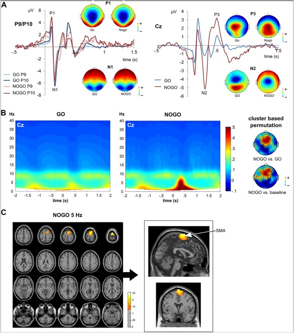
ERPs, TFT, and source reconstruction for GO and NOGO trials. (A) ERP data for GO und NOGO trials, shown in blue and red colors, respectively. Time point 0 denotes the onset of target stimulus presentation. The scalp topography plots show the voltage distribution across the scalp for each ERP component separately. Red colors denote positive potentials, blue colors denote negative potentials. Left: P1 and N1 ERPs at electrodes P9 and P10. Right: N2 and P3 ERPs at electrode Cz. (B) TFT power plots for GO and NOGO trials at electrode Cz. The y‐axis denotes frequency, the x‐axis denotes the time in ms relative to the stimulus onset. The scalp plots show the results of the non‐parametric cluster based permutation tests (5 Hz, 350–450 ms), by contrasting NOGO against GO trial activity or against baseline activity. Red colors denote positive power differences;, blue colors denote negative power differences. Electrodes belonging to significant positive clusters of electrodes are marked with a red cross. (C) Results of the DICS beamforming source reconstruction for NOGO trials at a central frequency of 5 Hz. The colors denote the difference of source power estimate ratios to baseline activity. All colors denote positive differences, that is, stronger activity compared with baseline activity. [Color figure can be viewed at http://wileyonlinelibrary.com]

The P1 ERP amplitude was significantly larger in NOGO trials (4.42 µV ± 2.77) than in GO trials (2.70 µV ± 2.09), as shown by a dependent samples t‐test (t[37] = −9.99; P < 0.001). In contrast, the N1 ERP was more negative in GO trials (–5.64 µV ± 3.40) than in NOGO trials (–4.54 µV ± 3.91) (t[37] = −3.90; P < 0.001). As indicated by a significant t‐test (t[37] = 5.98; P < 0.001), the N2 was larger, that is, more negative, in NOGO trials (–1.89 µV ± 2.79) than in GO trials (–0.77 µV ± 0.91). Additionally, the P3 ERP amplitude was significantly more positive in NOGO trials (0.76 µV/m² ± 1.56) than in GO trials (0.18 µV ± 0.83) (t[37] = −7.31; P < 0.001). There were no latency effects (all P ≥ 0.4). The results of the consecutive TFT analysis are shown in Figure 1B. As can be seen in Figure 1B, there was an activity peak in NOGO trials around 300–400 ms after target stimulus onset, which covered the theta frequency band from 4 to 7 Hz, with a power peak at about 5 Hz (4.75 Hz at 340 ms). This theta activity was not evident in the GO condition (refer Figure 1B; for a difference plot, please refer to Supporting information Fig. SB). To validate this difference in theta power, non‐parametric cluster‐based permutation tests were conducted, which contrasted NOGO and GO condition for the frequency range of 4–6 Hz. This test revealed a positive fronto‐central cluster of electrodes including electrodes Cz, FCz, and Fz (P < 0.002; see topoplots in Fig. 1B). Additionally, the theta activity increase in NOGO trials was compared with a baseline interval, revealing a positive fronto‐central cluster of electrodes (P < 0.002; refer to topoplots in Fig. 1B). Next, beamforming source reconstruction techniques were applied to analyze the source of the theta burst in the NOGO condition, which had a central frequency of 5 Hz (see Fig. 1C). The beamformer revealed that the estimated sources for the theta activity increase were located in a cluster of medial frontal regions including the left and right SFG (peak MNI coordinates in mm: −10/–9/80) and the SMA (0/1/80). To incorporate the whole theta frequency range from 4 to 7 Hz and to enable a comparison with the RIDE cluster analysis, beamforming source reconstruction was also applied to central frequencies at 4 and 7 Hz. The identified sources were similar to those of the 5Hz central frequency and comprised the SMA (4 and 7 Hz) and SFG (4 Hz) (please refer to the Supporting Information Fig. SA).

To dissociate stimulus and response selection processes in the EEG signal, the RIDE decomposition algorithm was applied to the time‐domain data. The results of the RIDE decomposition are shown in Figure 2A.

Figure 2.

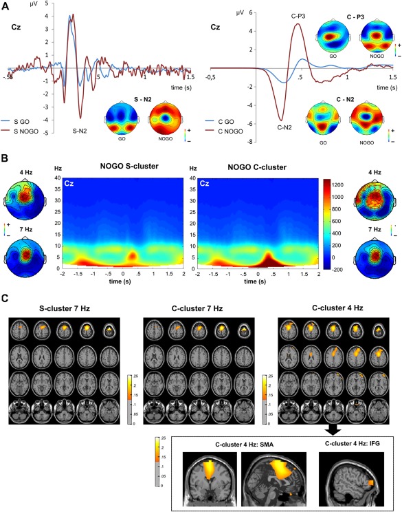
RIDE‐decomposed S‐ and C‐cluster data. (A) Waveforms showing the S‐cluster (left) and C‐cluster (right) decomposition of GO and NOGO trial data at electrode Cz. GO und NOGO trials are shown in blue and red colors, respectively. Time point 0 denotes the stimulus onset. The scalp topography plots separately show the voltage distribution across the scalp for each potential that resembles one of the ERPs from the undecomposed analysis. Red colors denote positive potentials, blue colors denote negative potentials. (B) TFT power plot for NOGO trials in the S‐cluster and C‐cluster at electrode Cz. The y‐axis denotes frequency, the x‐axis denotes the time in ms relative to the stimulus onset. The scalp plots separately show the results of the non‐parametric cluster based permutation tests for the S‐ and C‐cluster. The theta frequency power at 4 and 7 Hz in the time range of 350–450 ms was compared against baseline activity. Red colors denote positive power differences, blue colors denote negative differences. Electrodes belonging to significant positive clusters of electrodes are marked with a red cross. (C) Results of the DICS beamforming source reconstruction for the NOGO trial S‐ (4 and 7 Hz) and C‐cluster (4 Hz). The colors denote the difference of source‐power estimate ratios to baseline activity. All colors denote positive differences, that is, stronger activity compared with baseline activity. [Color figure can be viewed at http://wileyonlinelibrary.com]

The applied model decomposed the ERP data into an S‐cluster and a C‐cluster (see Fig. 2A). Based on visual inspection, both clusters showed a negative potential in the time window of the N2 ERP, but only the C‐cluster showed a positive potential in the time window of the P3. The consecutive analysis focused on NOGO trials only because we were mainly interested in inhibitory control processes. A TFT was applied to both clusters on NOGO trials. For the C‐cluster, strong theta band activity was found at about 300–400 ms after target stimulus presentation, with a maximum in the lower theta frequency band at about 4 Hz (power peak at 4 Hz, 371 ms), but extending to the upper theta frequency band (∼7 Hz). This matches the undecomposed data showing activity in the theta frequency from 4 to 7 Hz. For the S‐cluster, strong theta band activity was however also found at about 300–400 ms, but here, the power maximum was in the upper theta frequency band at about 7 Hz (7 Hz, 308 ms; for a difference plot please refer to Supporting Information Fig. SC). To validate these differences, cluster‐based permutation tests were conducted, which compared the 4 and 7 Hz theta activity in the time window of 300–400 ms for S‐ and C‐cluster separately. Additionally, theta activity was compared between S‐ and C‐cluster for 4 and 7 Hz frequency band separately. The results are depicted in Figure 2B. For all comparisons, a positive fronto‐central cluster of electrodes, including electrodes Cz and FCz, emerged (all P ≤ 0.024, see Figure 2B). Dependent‐samples t‐tests were used to compare the mean power of all electrodes within the identified electrodes cluster between the RIDE S‐cluster and C‐cluster for 4 and 7 Hz separately. For the 4 Hz frequency band, the power was significantly larger in the C‐cluster cluster (776.60 ± 604.08) than in the S‐cluster (560.02 ± 285.01) (t[37] = 2.98; P = 0.005). In contrast to this, theta power at 7 Hz did not differ significantly between S‐cluster (736.96 ± 609.20) and C‐cluster (743.53 ± 630.55) (t[37] = 0.319; P = 0.752). Most importantly, the S‐cluster theta activity was significantly larger at 7 than at 4 Hz (t[37] = −2.69; P = 0.011). No significant difference was found between 4 and 7 Hz in the C‐cluster (t[37] = −0.511; P = 0.612). Beamforming source reconstruction techniques were applied to determine the neuroanatomical sources of the modulations in the lower and upper theta activity band. Those analyses were separately conducted for the C‐cluster at 4 and 7 Hz as well as for the S cluster at 7 Hz. The results are shown in Figure 2C. Theta activity in the S‐cluster at 7 Hz was related to activity in the left and right SMA (0/1/80). Similar SMA sources (–1/1/73) were detected for 7 Hz theta activity in the C‐cluster. For 4 Hz in the C‐cluster, the beamformer determined sources in the left and right SMA (0/0/70). Yet and importantly, additional sources were found in frontal regions including the triangular part of the right inferior frontal gyrus (rIFG; 50/46/6).

DISCUSSION

In this study, we focused on the role of theta oscillations in inhibitory control. We examined whether there are distinguishable stimulus and response‐related processes (codes) and in how far these dissociable codes are processed in distinct functional neuroanatomical structures within the response inhibition network.

The results show that theta band activity was stronger in NOGO trials than in GO trials. This is well in line with the current literature [Beste et al., 2017, 2011; Dippel et al., 2016; Huster et al., 2013; Isabella et al., 2015; Quetscher et al., 2015] and suggests that cognitive control processes are enhanced during response inhibition. More importantly, we used RIDE on the EEG data to dissociate stimulus and response selection codes, which are reflected by the S and the C‐cluster, respectively [Mückschel et al., 2017; Ouyang et al., 2011]. The subsequent time frequency analysis of the S‐cluster (reflecting stimulus codes) revealed that the strongest oscillations were in the upper theta frequency band (∼7 Hz). Opposed to this, the time‐frequency decomposition of the C‐cluster (reflecting response selection codes) (Verleger et al., 2014) revealed that oscillations were strong in both the lower (∼4 Hz) and upper (∼7 Hz) theta frequency band. This may suggest that stimulus and response selection codes are gated via distinct oscillations within the theta frequency band. However, it needs to be noted that the differences found in the lower theta frequency band cannot be clearly dissociated from the upper part of the delta frequency band. Yet, theta frequency oscillations have been suggested to be important for cognitive control processes because stimulus and response selection processes need to be integrated (Cavanagh and Frank, 2014). This may well be achieved on the basis of codes in the theta frequency band because a large‐amplitude low‐frequency temporal scheme is ideal for organizing activities across large spatial distances (Buzsáki and Draguhn, 2004). This is a prerequisite for integrating sensory and response‐related processes during cognitive control (Cavanagh and Frank, 2014). It may be speculated that the concurrent coding of stimulus and response selection mechanisms within the same frequency band makes it easy to integrate these codes for goal‐directed behavior.

Notably, the beamforming analyses showed that concurrent stimulus and response selection codes in theta oscillations were processed in distinct cortical regions of the response inhibition network, that is, the SMA and the right inferior frontal cortex. For the S‐cluster, only one source was found in the SMA. Opposed to this, theta oscillations in the C‐cluster, which likely reflect response selection mechanisms between stimulus evaluation and responding [Mückschel et al., 2017; Verleger et al., 2014], were associated with the SMA as well as an area in the right inferior frontal cortex. The latter finding is in line with studies suggesting that the inferior frontal cortex supports an inhibition function during response inhibition processes [Aron et al., 2015, 2004; Garavan et al., 2006; Kelly et al., 2004; Konishi et al., 1998]. It has been argued that the (ventral) right inferior frontal cortex does not reflect attentional detection of an external signal [Aron et al., 2014], though this has not directly been shown. The finding that only theta oscillations of the C‐cluster, but not the S‐cluster, were associated with activation differences in right inferior frontal regions during inhibitory control (refer to Fig. 2) may be interpreted as that there is no stimulus‐related processing in inferior frontal regions. It seems that signals related to response selection processes (i.e., C‐cluster) are only evident in inferior frontal regions during inhibitory control. However, the data suggest that these signals are also evident in the SMA. This suggests that the “braking function”, or mechanisms important to inhibit automated response tendencies, are distributed across several areas of the response inhibition network. Given that the SMA has direct connections to the motor system and controls motor excitability independently from the primary motor cortex [Gerschlager et al., 2001; Rizzo et al., 2004] it seems reasonable that the SMA also processes response selection codes. This is further underlined by studies showing that the SMA is also involved in response initiation [Kawashima et al., 1996] and selection [Rowe et al., 2010] as well as inhibition [Nachev et al., 2005], which all underline a general role of the SMA in motor behavior and response selection [Mostofsky and Simmonds, 2008]. However, the finding that theta oscillations in the S‐cluster were also associated with the SMA, suggests that the SMA is involved in the processing of stimulus codes and response selection mechanisms. It may be speculated that the SMA serves as an interface between external stimulus codes and internal response selection codes. Response selection processes during inhibitory control may become informed by external signals via processes in the SMA. In line with this interpretation, it has recently been shown that different informational contents (codes) are processed in overlapping structures of the medial frontal cortex, including the SMA [Mückschel et al., 2017]. Because the SMA shows more direct structural connections to visual association areas than the inferior frontal cortex [Hagmann et al., 2008], it seems reasonable that the SMA, and not the inferior frontal cortex, seem to process stimulus codes and may serve such an interfacing function. Further in line with this interpretation, several lines of evidence have shown that medial frontal areas are affected by perceptual modulations of cognitive control [Labrenz et al., 2012; Westerhausen et al., 2010]; also during response inhibition processes [Bodmer and Beste, 2017]. However, this study focused on theta oscillation‐mediated processes and the results show that theta frequency oscillations showed strong differences between GO and Nogo trials, as well as between the different RIDE clusters.

Yet, future studies should further evaluate whether other oscillations (e.g., alpha frequency oscillations) are also modulated and also contain different informational content. This may be useful because especially posterior alpha dynamics reflect fluctuations in attentional selection processes that are known to contribute to performance in the applied experimental paradigm. In this regard, it should also be noted that even though the applied decomposition method allows to dissociate stimulus and response selection processes (codes) in the neurophysiological signal [Mückschel et al., 2017 ; Ouyang et al., 2011], especially the C‐cluster may still be heterogeneous and may require further decomposing [Ouyang et al., 2017]. So while the current study provides evidence that there are dissociable codes and associated functional neuroanatomical network during response inhibition, it is possible that the identified network can further be subdivided in the future.

In summary, the study suggests that there are distinct stimulus and response selection codes in theta oscillations during response inhibition processes. Notably, the results suggest that the functional neuroanatomical network associated with response inhibition processes can be subdivided with respect to the kind of codes that are processed within the theta frequency band. Although SMAs seem to process stimulus codes and response selection codes, the inferior frontal cortex only processes response selection codes.

Supporting information

Supporting Information.

REFERENCES

- Aron AR, Cai W, Badre D, Robbins TW (2015): Evidence supports specific braking function for inferior PFC. Trends Cogn Sci 19:711–712. [DOI] [PubMed] [Google Scholar]
- Aron AR, Robbins TW, Poldrack RA (2004): Inhibition and the right inferior frontal cortex. Trends Cogn Sci 8:170–177. [DOI] [PubMed] [Google Scholar]
- Aron AR, Robbins TW, Poldrack RA (2014): Inhibition and the right inferior frontal cortex: one decade on. Trends Cogn Sci 18:177–185. [DOI] [PubMed] [Google Scholar]
- Bari A, Robbins TW (2013): Inhibition and impulsivity: Behavioral and neural basis of response control. Prog Neurobiol 108:44–79. [DOI] [PubMed] [Google Scholar]
- Beste C, Mückschel M, Rosales R, Domingo A, Lee L, Ng A, Klein C, Münchau A (2017): Striosomal dysfunction affects behavioral adaptation but not impulsivity—Evidence from X‐linked dystonia‐parkinsonism. Mov Disord 32:576–584. [DOI] [PubMed] [Google Scholar]
- Beste C, Ness V, Falkenstein M, Saft C (2011): On the role of fronto‐striatal neural synchronization processes for response inhibition—Evidence from ERP phase‐synchronization analyses in pre‐manifest Huntington's disease gene mutation carriers. Neuropsychologia 49:3484–3493. [DOI] [PubMed] [Google Scholar]
- Bodmer B, Beste C (2017): On the dependence of response inhibition processes on sensory modality. Hum Brain Mapp 38:1941–1951. [DOI] [PMC free article] [PubMed] [Google Scholar]
- Boehler CN, Münte TF, Krebs RM, Heinze H‐J, Schoenfeld MA, Hopf J‐M (2009) Sensory MEG responses predict successful and failed inhibition in a stop‐signal task. Cereb Cortex N Y N 1991 19:134–145. [DOI] [PubMed] [Google Scholar]
- Buzsáki G, Draguhn A (2004): Neuronal Oscillations in Cortical Networks. Science 304:1926–1929. [DOI] [PubMed] [Google Scholar]
- Cavanagh JF, Frank MJ (2014): Frontal theta as a mechanism for cognitive control. Trends Cogn Sci 18:414–421. [DOI] [PMC free article] [PubMed] [Google Scholar]
- Chmielewski WX, Beste C (2016a): Perceptual conflict during sensorimotor integration processes—A neurophysiological study in response inhibition. Sci Rep 6:26289. [DOI] [PMC free article] [PubMed] [Google Scholar]
- Chmielewski WX, Beste C (2016b): Testing interactive effects of automatic and conflict control processes during response inhibition ‐ A system neurophysiological study. NeuroImage [DOI] [PubMed] [Google Scholar]
- Diamond A (2013): Executive functions. Annu Rev Psychol 64:135–168. [DOI] [PMC free article] [PubMed] [Google Scholar]
- Dippel G, Chmielewski W, Mückschel M, Beste C (2016): Response mode‐dependent differences in neurofunctional networks during response inhibition: an EEG‐beamforming study. Brain Struct Funct 221:4091–4101. [DOI] [PubMed] [Google Scholar]
- Dippel G, Mückschel M, Ziemssen T, Beste C (2017): Demands on response inhibition processes determine modulations of theta band activity in superior frontal areas and correlations with pupillometry – Implications for the norepinephrine system during inhibitory control. NeuroImage 157:575–585. [DOI] [PubMed] [Google Scholar]
- Duncan J (2010): The multiple‐demand (MD) system of the primate brain: mental programs for intelligent behaviour. Trends Cogn Sci 14:172–179. [DOI] [PubMed] [Google Scholar]
- Garavan H, Hester R, Murphy K, Fassbender C, Kelly C (2006): Individual differences in the functional neuroanatomy of inhibitory control. Brain Res 1105:130–142. [DOI] [PubMed] [Google Scholar]
- Gerschlager W, Siebner HR, Rothwell JC (2001): Decreased corticospinal excitability after subthreshold 1 Hz rTMS over lateral premotor cortex. Neurology 57:449–455. [DOI] [PubMed] [Google Scholar]
- Gross J, Kujala J, Hämäläinen M, Timmermann L, Schnitzler A, Salmelin R (2001): Dynamic imaging of coherent sources: Studying neural interactions in the human brain. Proc Natl Acad Sci U S A 98:694–699. [DOI] [PMC free article] [PubMed] [Google Scholar]
- Hagmann P, Cammoun L, Gigandet X, Meuli R, Honey CJ, Wedeen VJ, Sporns O (2008): Mapping the structural core of human cerebral cortex. PLOS Biol 6:e159. [DOI] [PMC free article] [PubMed] [Google Scholar]
- Hampshire A, Sharp DJ (2015): Contrasting network and modular perspectives on inhibitory control. Trends Cogn Sci 19:445–452. [DOI] [PubMed] [Google Scholar]
- Hoffmann S, Beste C (2015): A perspective on neural and cognitive mechanisms of error commission. Front Behav Neurosci 9: Available at: http://journal.frontiersin.org/article/10.3389/fnbeh.2015.00050/abstract [Accessed March 16, 2017]. [DOI] [PMC free article] [PubMed] [Google Scholar]
- Huster RJ, Enriquez‐Geppert S, Lavallee CF, Falkenstein M, Herrmann CS (2013): Electroencephalography of response inhibition tasks: Functional networks and cognitive contributions. Int J Psychophysiol 87:217–233. [DOI] [PubMed] [Google Scholar]
- Isabella S, Ferrari P, Jobst C, Cheyne JA, Cheyne D (2015): Complementary roles of cortical oscillations in automatic and controlled processing during rapid serial tasks. NeuroImage 118:268–281. [DOI] [PubMed] [Google Scholar]
- Kawashima R, Itoh H, Ono S, Satoh K, Furumoto S, Gotoh R, Koyama M, Yoshioka S, Takahashi T, Takahashi K, Yanagisawa T, Fukuda H (1996): Changes in regional cerebral blood flow during self‐paced arm and finger movements. A PET study. Brain Res 716:141–148. [DOI] [PubMed] [Google Scholar]
- Kelly AMC, Hester R, Murphy K, Javitt DC, Foxe JJ, Garavan H (2004): Prefrontal‐subcortical dissociations underlying inhibitory control revealed by event‐related fMRI. Eur J Neurosci 19:3105–3112. [DOI] [PubMed] [Google Scholar]
- Konishi S, Nakajima K, Uchida I, Sekihara K, Miyashita Y (1998): No‐go dominant brain activity in human inferior prefrontal cortex revealed by functional magnetic resonance imaging. Eur J Neurosci 10:1209–1213. [DOI] [PubMed] [Google Scholar]
- Labrenz F, Themann M, Wascher E, Beste C, Pfleiderer B (2012): Neural correlates of individual performance differences in resolving perceptual conflict. PloS One 7:e42849. [DOI] [PMC free article] [PubMed] [Google Scholar]
- Maris E, Oostenveld R (2007): Nonparametric statistical testing of EEG‐ and MEG‐data. J Neurosci Methods 164:177–190. [DOI] [PubMed] [Google Scholar]
- Mostofsky SH, Simmonds DJ (2008): Response inhibition and response selection: two sides of the same coin. J Cogn Neurosci 20:751–761. [DOI] [PubMed] [Google Scholar]
- Mückschel M, Chmielewski W, Ziemssen T, Beste C (2017): The norepinephrine system shows information‐content specific properties during cognitive control – Evidence from EEG and pupillary responses. NeuroImage 149:44–52. [DOI] [PubMed] [Google Scholar]
- Mückschel M, Stock A‐K, Beste C (2014): Psychophysiological mechanisms of interindividual differences in goal activation modes during action cascading. Cereb Cortex 24:2120–2129. [DOI] [PubMed] [Google Scholar]
- Mückschel M, Stock A‐K, Dippel G, Chmielewski W, Beste C (2016): Interacting sources of interference during sensorimotor integration processes. NeuroImage 125:342–349. [DOI] [PubMed] [Google Scholar]
- Nachev P, Rees G, Parton A, Kennard C, Husain M (2005): Volition and conflict in human medial frontal cortex. Curr Biol 15:122–128. [DOI] [PMC free article] [PubMed] [Google Scholar]
- Nigbur R, Ivanova G, Stürmer B (2011): Theta power as a marker for cognitive interference. Clin Neurophysiol 122:2185–2194. [DOI] [PubMed] [Google Scholar]
- Oostenveld R, Fries P, Maris E, Schoffelen J‐M (2010): FieldTrip: Open source software for advanced analysis of MEG, EEG, and invasive electrophysiological data. Comput Intell Neurosci 2011:e156869. [DOI] [PMC free article] [PubMed] [Google Scholar]
- Oostenveld R, Stegeman DF, Praamstra P, van Oosterom A (2003): Brain symmetry and topographic analysis of lateralized event‐related potentials. Clin Neurophysiol off J Int Fed Clin Neurophysiol 114:1194–1202. [DOI] [PubMed] [Google Scholar]
- Ouyang G, Herzmann G, Zhou C, Sommer W (2011): Residue iteration decomposition (RIDE): A new method to separate ERP components on the basis of latency variability in single trials. Psychophysiology 48:1631–1647. [DOI] [PubMed] [Google Scholar]
- Ouyang G, Hildebrandt A, Sommer W, Zhou C (2017): Exploiting the intra‐subject latency variability from single‐trial event‐related potentials in the P3 time range: A review and comparative evaluation of methods. Neurosci Biobehav Rev 75:1–21. [DOI] [PubMed] [Google Scholar]
- Ouyang G, Schacht A, Zhou C, Sommer W (2013): Overcoming limitations of the ERP method with Residue Iteration Decomposition (RIDE): A demonstration in go/no‐go experiments. Psychophysiology 50:253–265. [DOI] [PubMed] [Google Scholar]
- Ouyang G, Sommer W, Zhou C (2015a): A toolbox for residue iteration decomposition (RIDE)—A method for the decomposition, reconstruction, and single trial analysis of event related potentials. J Neurosci Methods 250:7–21. [DOI] [PubMed] [Google Scholar]
- Ouyang G, Sommer W, Zhou C (2015b): Updating and validating a new framework for restoring and analyzing latency‐variable ERP components from single trials with residue iteration decomposition (RIDE). Psychophysiology 52:839–856. [DOI] [PubMed] [Google Scholar]
- Quetscher C, Yildiz A, Dharmadhikari S, Glaubitz B, Schmidt‐Wilcke T, Dydak U, Beste C (2015): Striatal GABA‐MRS predicts response inhibition performance and its cortical electrophysiological correlates. Brain Struct Funct 220:3555–3564. [DOI] [PMC free article] [PubMed] [Google Scholar]
- Rizzo V, Siebner HR, Modugno N, Pesenti A, Münchau A, Gerschlager W, Webb RM, Rothwell JC (2004): Shaping the excitability of human motor cortex with premotor rTMS. J Physiol 554:483–495. [DOI] [PMC free article] [PubMed] [Google Scholar]
- Robertson IH, Manly T, Andrade J, Baddeley BT, Yiend J (1997): ‘Oops!’: Performance correlates of everyday attentional failures in traumatic brain injured and normal subjects. Neuropsychologia 35:747–758. [DOI] [PubMed] [Google Scholar]
- Rowe JB, Hughes L, Nimmo‐Smith I (2010): Action selection: a race model for selected and non‐selected actions distinguishes the contribution of premotor and prefrontal areas. NeuroImage 51:888–896. [DOI] [PMC free article] [PubMed] [Google Scholar]
- Stock A‐K, Popescu F, Neuhaus AH, Beste C (2016): Single‐subject prediction of response inhibition behavior by event‐related potentials. J Neurophysiol 115:1252–1262. [DOI] [PMC free article] [PubMed] [Google Scholar]
- Töllner T, Wang Y, Makeig S, Müller HJ, Jung T‐P, Gramann K (2017): Two independent frontal midline theta oscillations during conflict detection and adaptation in a simon‐type manual reaching task. J Neurosci 37:2504–2515. [DOI] [PMC free article] [PubMed] [Google Scholar]
- Verleger R, Metzner MF, Ouyang G, Śmigasiewicz K, Zhou C (2014): Testing the stimulus‐to‐response bridging function of the oddball‐P3 by delayed response signals and residue iteration decomposition (RIDE). NeuroImage 100:271–280. [DOI] [PubMed] [Google Scholar]
- Westerhausen R, Moosmann M, Alho K, Belsby S‐O, Hämäläinen H, Medvedev S, Specht K, Hugdahl K (2010): Identification of attention and cognitive control networks in a parametric auditory fMRI study. Neuropsychologia 48:2075–2081. [DOI] [PubMed] [Google Scholar]
Associated Data
This section collects any data citations, data availability statements, or supplementary materials included in this article.
Supplementary Materials