Uncovering phase‐coupled oscillatory networks in electrophysiological data

Abstract

Phase consistent neuronal oscillations are ubiquitous in electrophysiological recordings, and they may reflect networks of phase‐coupled neuronal populations oscillating at different frequencies. Because neuronal oscillations may reflect rhythmic modulations of neuronal excitability, phase‐coupled oscillatory networks could be the functional building block for routing information through the brain. Current techniques are not suited for directly characterizing such networks. To be able to extract phase‐coupled oscillatory networks we developed a new method, which characterizes networks by phase coupling between sites. Importantly, this method respects the fact that neuronal oscillations have energy in a range of frequencies. As a consequence, we characterize these networks by between‐site phase relations that vary as a function of frequency, such as those that result from between‐site temporal delays. Using human electrocorticographic recordings we show that our method can uncover phase‐coupled oscillatory networks that show interesting patterns in their between‐site phase relations, such as travelling waves. We validate our method by demonstrating it can accurately recover simulated networks from a realistic noisy environment. By extracting phase‐coupled oscillatory networks and investigating patterns in their between‐site phase relations we can further elucidate the role of oscillations in neuronal communication. Hum Brain Mapp 36:2655–2680, 2015. © 2015 Wiley Periodicals, Inc.

INTRODUCTION

Oscillations are a prominent feature of neuronal signals [Buzsaki and Draguhn, 2004]. When measured at multiple sites, these site‐specific signals are very often phase consistent. As these sites may measure multiple sources, they can reflect phase‐coupled oscillatory networks. Because oscillations may reflect rhythmic modulations of neuronal excitability [Buzsaki et al., 2012; Fries, 2005], phase‐coupled oscillatory networks could be the functional building block for routing of information in the brain [for reviews see Palva and Palva, 2012; Schnitzler and Gross, 2005; Siegel et al., 2012]. These networks will overlap at least partially in space, frequency and time, forming a complex structure in which the routing of information depends on phase relations at multiple frequencies [Akam and Kullmann, 2014; Canolty et al., 2010; Canolty and Knight, 2010; Miller et al., 2012; Schyns et al., 2011; van der Meij et al., 2012].

Networks of functionally connected brain regions have been studied for more than a decade using the hemodynamic response measured by functional magnetic resonance imaging [fMRI; for a review see Deco and Corbetta, 2011]. Networks of coupled sites have also been found using electrophysiological signals, on the basis of correlations between envelopes of oscillatory amplitudes at different frequencies [Brookes et al., 2011; de Pasquale et al., 2010; Hipp et al., 2012]. Crucially, between‐site amplitude envelope correlations do not reflect between‐site phase consistency, and therefore, cannot be interpreted in terms of phase‐coupled fluctuations of neuronal excitability.

Characterizing coupling between sites using fluctuations in neuronal excitability with existing methods is a tremendous challenge if there are no strong hypotheses about which neuronal populations are likely to interact. This is because existing methodology is based on pair‐wise measures, such as coherence [Rosenberg et al., 1998], Granger‐causality [Bernasconi and Konig, 1999], phase‐locking value [Lachaux et al., 1999], and others. Such measures quantify the strength and/or direction of phase coupling at the level of site‐pairs, and therefore, do not reveal the spatial distribution of phase‐coupled networks, at least not without prior information about a seed region and the frequency band in which this phase‐coupling occurs.

To investigate phase‐coupled oscillatory networks it is crucial to appreciate the fact that brain rhythms have energy in a range of frequencies. This has important implications for the between‐site phase relations. For instance, networks with consistent between‐site time delays have between‐site phase relations that are a linear function of frequency. We developed a new method that is capable of extracting such networks from electrophysiological data.

In the following, we present, apply and validate a method that extracts phase‐coupled oscillatory networks. This method is grounded in a plausible model of a neurobiological rhythm: a spatially distributed oscillation with energy in a range of frequencies and involving between‐site phase relations that vary as a function of frequency. The method is useful because electrophysiological data almost always involve multiple networks, overlapping in both space and frequency. Our method separates these networks and characterizes them in a neurobiologically informative way. To demonstrate that our method works we apply it real data, and validate it using simulations. Using ECoG recordings we show that it is capable of uncovering networks and characterizing them in an informative way. Using simulated data we show that it is capable of uncovering ground truth networks in the context of neurobiologically realistic noise.

MATERIALS AND METHODS

Extracting Phase‐Coupled Oscillatory Networks Using SPACE

To extract phase‐coupled oscillatory networks we developed a new decomposition technique, denoted as Spatially distributed PhAse Coupling Extraction (for SPACE). It is inspired by complex‐valued PARAFAC [Bro, 1998; Carrol and Chang, 1970; Harshman, 1970; Sidiropoulos et al., 2000]. In this section, we provide a brief introduction into the method. A full description of the method and the underlying algorithm is provided in the Appendix.

We extract phase‐coupled oscillatory networks using two models: the time delay model and the Frequency‐Specific Phases model (for FSP). Both models follow our characterization of phase‐coupled oscillatory networks presented in the Results Section and extract networks that consist of a frequency profile, a spatial amplitude map, an epoch profile, and an array of phase offsets. The time delay model (SPACE‐time) describes phase relations between sites by temporal delays between sites, in a spatial time‐delay map. The FSP model (SPACE‐FSP) describes these phase relations by FSP, in spatial phase maps. Below, we present both models in more detail. The two models are complementary. The time delay model is capable of directly revealing the temporal structure of, traveling waves, and is therefore, suited for targeted analyses of temporal dynamics. The FSP model can extract networks with any kind of phase structure, and is therefore most useful in explorative analyses. Both models extract networks from a three‐way array of Fourier coefficients $X_{jkl}$, with dimensionality sites ( $J$), frequencies ( $K$), and epochs ( $L$), obtained from a spectral analysis of electrophysiological recordings. Phase‐coupled oscillatory networks can partially overlap in their spatial configuration, spectral content, and temporal pattern. Our method separates such networks by their different structure over the spatial, spectral and temporal dimensions of the input array, that is, on the basis of their different spatial maps, frequency profiles, and epoch profiles.

The time delay model (Fig. 1A; see Appendix) is formulated as follows in element‐wise notation:

$$\text{SPACE}-\text{time}: X_{jkl}= {\displaystyle \sum }_{f=1}^F{a}_{jf}\cdot \text{exp}\left(i2\pi {\phi }_k{\sigma }_{jf}\right)\cdot b_{kf}\cdot c_{lf}\cdot \text{exp}\left(i2\pi {\tau }_{klf}\right)+{\varepsilon }_{jkl}$$

Figure 1.

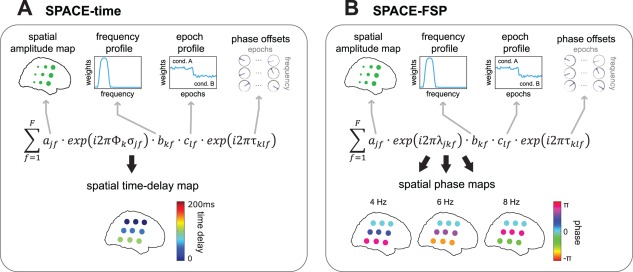
SPACE: describing phase‐coupled oscillatory networks by FSP and time delays. We developed a new decomposition technique that extracts phase‐coupled oscillatory networks, SPACE. Networks are extracted using two models, the time delay model and the FSP model. The time delay model (SPACE‐time) describes phase relations between sites by temporal delays between sites, in a spatial time‐delay map. The FSP model (SPACE‐FSP) describes these phase relations by FSP, in spatial phase maps. A: The time delay model describes networks by a spatial amplitude map, a frequency profile, a spatial time‐delay maps, an epoch profile, and phase offsets. The equation in A is the element‐wise formulation of the time delay model, and it shows how each Fourier coefficients $X_{jkl}$ of site $j$, frequency $k$, and epoch $l$ is described. The example shows the same network as in Figure 3. The time‐delay maps describe all phase differences by site‐specific time delays. In the example, each site row has a time delay of 50 ms from top to bottom. These 50 ms steps produce the same phases as shown in B, and match the time delays in Figure 3A. B: The FSP model describes networks by a spatial amplitude map, a frequency profile, an epoch profile, phase offsets, and frequency‐specific spatial phase maps. The spatial phase maps describe all phase differences between sites, matching those in Figure 3A. No constraint is placed on phases over frequencies, in contrast to the time delay model. For a detailed description see Materials and Methods and Results Section: Characterizing Phase‐Coupled Oscillatory Networks In Terms of Frequency Profiles, Spatial Maps, and Epoch Profiles. [Color figure can be viewed in the online issue, which is available at http://wileyonlinelibrary.com.]

The Fourier coefficient $X_{jkl}$ is described as a sum over $F$ network‐specific complex‐valued numbers. The amplitude of each network‐specific complex‐valued number is the product of $a_{jf}$, $b_{kf}$, and $c_{lf}$, which refer to, respectively, the spatial amplitude map, the frequency profile and the epoch profile. The phase of each network‐specific complex‐valued number is the product of an element of the spatial time‐delay map and a phase offset: $\text{exp}\left(i2\pi {\phi }_k{\sigma }_{jf}\right)$ and $\text{exp}\left(i2\pi {\tau }_{klf}\right)$. Here, $2\pi {\phi }_k{\sigma }_{jf}$ describes the site‐, frequency‐, and network‐specific phases, in which ${\phi }_k$ denotes the $k$‐th frequency (in Hz) and ${\sigma }_{jf}$ denotes the site‐ and frequency‐specific time delay. $2\pi {\tau }_{klf}$ describes the frequency‐, epoch‐, and network‐specific phase offset. The time delay model is based on the assumption that between‐site phase differences are the result of between‐site time delays. To make this concrete, let $\sigma$ be the time delay between two sites and let $\phi$ be frequency. Then, the between‐site phase difference is $\phi \cdot \sigma$, which increases linearly with frequency. In the FSP model (Fig. 1B; see Appendix), the spatial phase maps replace the spatial time‐delay maps. For this model, the phase of each network‐specific complex‐valued number is the product of an element of the spatial phase maps and a phase offset: $\text{exp}\left(i2\pi {\lambda }_{jkf}\right)$ and $\text{exp}\left(i2\pi {\tau }_{klf}\right)$. The FSP model is formulated as follows in element‐wise notation:

$$\text{SPACE}‐\text{FSP}: X_{jkl}= \sum _{f=1}^F{a}_{jf}\cdot \text{exp}\left(i2\pi {\lambda }_{jkf}\right)\cdot b_{kf}\cdot c_{lf}\cdot \text{exp}\left(i2\pi {\tau }_{klf}\right)+{\varepsilon }_{jkl}$$

Except for the site‐, frequency‐ and network‐specific phases ${\lambda }_{jkf}$, this model has the same parameters as the time delay model. In contrast to the time delay model, no constraints are imposed on the between‐site phase differences as a function of frequency. The parameters of both models can be estimated using an alternating least squares (ALS) algorithm, which monotonically decreases a least squares (LS) loss function. For this algorithm, new optimization techniques were developed which are fully described in the Appendix.

To be estimable, all parameters of the two models have to be normalized (see Appendix). Because of this normalization, the individual amplitudes $a_{jf}$, $b_{kf}$, $c_{lf}$, and the individual phases/time delays ${\lambda }_{jkf}$, ${\sigma }_{jf}$, are not meaningful. Crucially, however, amplitude ratios, and time delay differences and phase differences between sites, frequencies, and epochs, are not affected by these normalizations, and reveal important characteristics of the extracted phase‐coupled oscillatory networks.

In the three‐way array of Fourier coefficients, every epoch is described by a single Fourier coefficient per site and frequency. However, it is often desired to control the frequency resolution by means of multitaper estimation. When using multitaper estimation, every epoch has multiple tapers, and each of these tapers produces one Fourier coefficient. These taper‐specific Fourier coefficients are organized in an additional dimension, turning the three‐way array into a four‐way array of Fourier coefficients. However, because frequencies and epochs can differ in their number of tapers, this four‐way array may be partially empty, and the three‐way formulation of the models cannot accommodate this aspect of the data array. Fortunately, we can make use of the cross‐product formulation of our models to deal with this. This is the formulation of the models that is used in the remainder of the article, and it is fully described in the Appendix. Crucially, the cross‐product formulation does not affect the spatial amplitude maps, the frequency profiles, the epoch profiles, nor the spatial phase maps or spatial time‐delay maps, as described above and in the Results Section. The phase offsets, however, are parameterized differently (see Appendix). An important difference with the models for the three‐ and four‐way arrays of Fourier coefficients is that in the cross‐product formulation of these models, between‐network coherence is explicitly modeled. Although this can be of great benefit, it also has an undesirable consequence: if the between‐network coherences are treated as estimable parameters, then a distributed phase‐coupled oscillatory network can be described by an arbitrary number of coherent subnetworks. To avoid this, we force between‐network coherence to be zero (see Appendix).

The number of networks $F$ that are extracted needs to be estimated. The number of networks that should be extracted cannot be determined analytically. To find the optimal $F$, we can make use of an index of the reliability with which the networks can be estimated from the data, as described by Maris et al. [2011].The number of networks that are extracted can be increased incrementally until this reliability index drops below a preset level. A conservative approach is to split the data into two halves, extract networks from both halves, and stop increasing the number of networks when they start to differ between halves. We use this approach for analyzing the ECoG data, and it is described in detail below. Other methods of estimating the optimal $F$ are also possible [see Bro, 1998, for examples from the perspective of PARAFAC/2].

Experimental Paradigm and Preprocessing of ECoG Recordings

Three pharmacoresistant epilepsy patients (1 male, 2 female) were implanted with subdural grid and strip electrodes prior to undergoing resective surgery. Informed consent was obtained from the patients or their guardians if they were underage. The research protocol was approved by the appropriate institutional review boards at the Children's Hospital (Philadelphia, PA) and the University Clinic (Freiburg, Germany). Some of the datasets have been analyzed before [see e.g., Jacobs and Kahana, 2009; Maris et al., 2011; Raghavachari et al., 2006; Rizzuto et al., 2003; van der Meij et al., 2012; van Vugt et al., 2010]. Patients performed a Sternberg working memory task [Sternberg, 1966] while ECoG recordings were obtained. Patients were presented with a series of letters (with variable length from 1 to 6) on a computer screen, and they were instructed to remember these. The trial started with the presentation of a fixation cross, followed by a letter for 700 ms and by 275–350 ms (uniformly distributed) of blank screen. Every additional letter was presented for 700 ms and followed by 275–350 ms of blank screen, except for the last letter which was followed by a reten tion in terval of 425–575 ms (uniformly distributed as well). After the retention interval, a probe letter was presented. Patients were required to indicate by means of key press whether the probe letter was part of the previously presented letter series. We analyzed the period between the fixation cross and the onset of the probe letter, a period during which the patients were actively engaged in the task. We did not distinguish between the cognitive operations encoding and retrieval, which occur in this period. The main purpose of the current analyses was to demonstrate that plausible phase‐coupled oscillatory networks can be extracted.

ECoG recordings were sampled at 256 Hz and rereferenced to the common average. Artifact rejection was performed by visual inspection. All trials and/or electrodes contaminated by epileptiform activity were removed. The data was band‐stop filtered with 1 Hz windows at 50 and 60 Hz (depending on continent) and at other frequencies containing line noise. Recordings were additionally band‐pass filtered between 0.01 and 100 Hz. All filters were fourth‐order Butterworth. Subsequently, the mean and the linear trend were removed from each trial. To suppress the 1/f^x pattern in the power spectrum, the data was prewhitened by taking the first temporal derivative. Electrode locations were determined by coregistering a postoperative computed tomography scan with a higher resolution preoperative magnetic resonance image. Patients' brains were normalized to Talairach space [Talairach and Tornoux, 1988]. All preprocessing and spectral analysis was performed using custom analyses scripts and the FieldTrip open‐source MATLAB toolbox [Oostenveld et al., 2011].

Extracting Phase‐Coupled Oscillatory Networks from ECoG Recordings

Spectral analysis was performed for 2–30 Hz with equally spaced 0.5 Hz bins and a Welch multitapering approach [Welch, 1967] to control frequency resolution. First, each trial was cut into several 2 second segments, such that each next segment would have a temporal overlap of 75% with the previous segment (incomplete segments at the end of a trial were not used). Each of the 2 second segments was multiplied with a Hanning window, followed by a Discrete Fourier Transform (DFT). These multiple 2 second segments of each trial are the separate Welch tapers. Each epoch used in the analyses corresponds to three consecutive trials and we combined the Fourier coefficients obtained from these trials. This resulted in 30 epochs out of 92 trials for patient 1, 54 epochs out of 163 trials for patient 2, and 89 epochs out of 270 trials from patient 3. Combining tapers of multiple trials was necessary because our method requires that the smallest number of tapers per epoch is larger than the number of networks extracted. Because we wanted to estimate the number of networks using a high frequency resolution, this sometimes lead to a larger number of networks than tapers when defining each trial as an epoch.

The same preprocessing procedure was used for displaying single trials at the peak frequency of the example networks (see Results Section). The resulting time series were then convolved with a complex‐valued wavelet at the selected frequencies. This wavelet was constructed by an element‐wise multiplication of a three‐cycle complex exponential and a Hanning taper of equal length. The real part of the resulting complex‐valued time series was then used for display.

Fourier coefficients resulting from spectral analysis were arranged to form a four‐way array and decomposed using the cross‐product formulation of both SPACE‐time and SPACE‐FSP (see Appendix). To avoid local minima, each algorithm was randomly initialized 20 times, and the solution with the highest explained variance was selected (explained variance over initializations is shown in Supporting Information Fig. S1). To avoid degenerate decompositions from unfortunate initializations, all decompositions were run with an orthogonality constraint ( $D_k=I$; see Appendix). The number of networks to extract (four, two, and four for patient 1, 2, and 3, respectively) was determined on the basis of a split‐half approach using the output of SPACE‐time. In this procedure, the number of networks was increased until the networks extracted from the odd numbered trials were no longer similar enough to the networks extracted from the even numbered trials. As such, the number of networks that is extracted depends on the networks that are consistently activated by the task. Similarity was evaluated on the basis of a number of split‐half reliability coefficients. One coefficient was calculated for each of the parameter sets.

This split‐half reliability coefficient was computed for the spatial amplitude map and the frequency profiles as the normalized network‐specific inner‐product. For the spatial time‐delay maps, the split‐half reliability coefficient was constructed in two steps:

$$\text{split}-\text{half} \text{coefficient}: \frac{{\sum }_{k=1}^K\left[\left|\frac{<A^1\cdot \text{exp}\left(i2\pi {\phi }_k{\sigma }^1\right), A^2\cdot \text{exp}\left(i2\pi {\phi }_k{\sigma }^2\right)>}{A^1\cdot A^2}\right|\cdot \frac{B_k^1+B_k^2}{2}\right]}{{\sum }_{k=1}^K\left[\frac{B_k^1+B_k^2}{2}\right]}$$ (1)

First, per split‐half $s$ and frequency $k$, a complex‐valued spatial time‐delay map $\text{exp}\left(i2\pi {\phi }_k{\sigma }^s\right)$ was computed and weighted with the split‐half specific spatial amplitude map $A^s$. Then, the normalized inner‐product $〈,〉$ was taken between both halves. The final reliability coefficient for the spatial time‐delay maps was then constructed by computing the average over frequencies of the absolute value (denoted by $\left|\right|$) of this inner‐product, weighted by the average of the frequency profiles $B_k^s$ of both split‐halves. For the spatial phase maps, the reliability coefficient was constructed by replacing ${\phi }_k{\sigma }^s$ by ${\lambda }_k^s$ in the above equation. When either this coefficient or that of the spatial amplitude map or the frequency profile fell below 0.7, the procedure was stopped, and the previous number of networks was set as the final number of networks. As $D_k=I$, it was not part of the split‐half reliability coefficient.

We additionally computed a similarity coefficient that was used to compare networks extracted using the time delay model to networks extracted using the FSP model. This coefficient was similar to the split‐half coefficient described above. For the spatial amplitude map, the frequency profiles, and the epoch profile the coefficient was computed as the normalized inner‐product. For the spatial time‐delay map and the spatial phase maps the coefficient was constructed as in Eq. (1), except that the spatial time‐delay map of the second network $\text{exp}\left(i2\pi {\phi }_k{\sigma }^2\right)$ was replaced by the spatial phase maps $\text{exp}\left(i2\pi {\lambda }_k^2\right)$. The similarity coefficient for the whole network was then obtained as the average of the coefficients for spatial amplitude map, the spatial phase map, the frequency profile, and the epoch profile.

Simulating Phase‐Coupled Oscillatory Networks

To show that both our method is capable of extracting networks from noisy data we simulated three phase‐coupled oscillatory networks travelling over a 5 × 5 sites grid. Each network had a spatial amplitude map that was nonzero for a selected set of sites, with overlap between the networks. There was one network in the theta range (4–8 Hz), one in the alpha range (8–12 Hz), and one in the beta range (10–25 Hz). Every network was present in 15 out of 25 epochs, with overlap between the epochs. Per epoch, we generated a signal that propagated over the involved sites with a fixed time delay, thus forming a travelling wave. The time delay step size (i.e., the time delay between two adjacent sites) was systematically varied over the values 5, 25, 50, and 100 ms. We additionally varied the signal‐to‐noise ratio (SNR) and the spatial noise correlation, as described below.

The signal was generated as follows. First, 1.5 (theta) or 1 s (alpha and beta) of white noise was generated using MATLAB's pseudorandom number generator. Then, after taking the DFT, all Fourier coefficients not belonging to the network's frequency band were set to zero. Subsequently, the signal was transformed back to the time domain using the inverse DFT, and the resulting signal was multiplied with a Hanning window of equal length and padded out to 3 s. This resulted in an oscillatory signal within the specified frequency band. Then, again using a DFT, the amplitudes of the Fourier coefficients were scaled such the amplitude spectrum was proportional to 1/f, giving the power spectrum a 1/f ² shape [Miller et al., 2009]. The resulting signal was then transformed back to the time domain using the inverse DFT. The site‐specific signals were obtained by shifting this time domain signal in accordance with the order of the site in travelling wave and the time delay step size. To every site, we added 3 s of noise. These noise signals were generated in the same way as the source signals but without the removal of particular frequencies, and independently for each site. We varied the amount of spatial noise correlation by generating new site‐specific noise signals as a weighted average of the initial noise signals. These weights were proportional to a bivariate Gaussian of which the full‐width half maximum [the width of the Gaussian at the point where its magnitude is at the half of its maximum; full‐width half‐maximum (FWHM)] was systematically varied over the values 0, 10, 20, and 40 mm (simulated sites were spaced 10 mm apart). This results in a FWHM that encompassed 0, 3, 5, and 9 sites, respectively. We also systematically varied noise strength. This was achieved in a final step by setting the SNR of the time series at each site to be 4, 0.16, 0.04, or 0.01.

Analyzing the Simulated Data

Except for artifact removal, the simulated data were preprocessed in the same way as the ECoG data. First, the mean and the linear trend were removed from each epoch. Next, to suppress the 1/f^x shape of the power spectrum, the data was prewhitened by taking the first temporal derivative.

Spectral analysis was performed for 2–30 Hz with equally spaced 1 Hz bins. First, each 3 second epoch was cut into several 1 second segments, such that each next segment would have a temporal overlap of 75% with the previous segment. For 2–16 Hz, each of the 1 second segments was multiplied with a Hanning window, followed by a DFT. For 17–30 Hz, each segment of each epoch was multiplied several times with different tapers prior to taking the DFT. These tapers were the first 3 tapers of the Slepian sequence [Percival and Walden, 1993] of order 4, resulting in a frequency resolution of approximately 2 Hz.

The Fourier coefficients of all segments were then collected per epoch, and arranged in a four‐way array. This array consisted of 25 sites, 29 frequencies, 25 epochs, and 57 tapers for every simulation run. Each four‐way array of Fourier coefficients resulting from one simulation run was decomposed using the cross‐product formulations of both SPACE‐time and SPACE‐FSP. To avoid local minima, each algorithm was randomly initialized 10 times, of which the solution with the highest explained variance was retained (explained variance over initializations is shown in Supporting Information Fig. S1). As for the analyses of the ECoG data, all decompositions were run with an orthogonality constraint ( $D_k=I$; see above). All preprocessing and spectral analysis was performed using custom analyses scripts and the FieldTrip open‐source MATLAB toolbox [Oostenveld et al., 2011].

Coefficients for Evaluating the Goodness‐of‐Recovery of the Simulated Networks

We calculated a number of coefficients to assess the goodness‐of‐recovery of the simulated networks. We use four different coefficients: (1) one for the spatial amplitude maps, frequency profiles and epoch profiles, (2) one for the spatial phase maps, (3) one for the spatial time‐delay maps, and (4) one for the temporal order of the time delays. The first coefficient is the Pearson correlation coefficient, which ranges from −1 to 1. The other three coefficients were constructed for the purpose of this study, and will be described in more detail in the following. Each of the four coefficients was computed per network and per simulation run and subsequently averaged.

The recovery coefficient for a network‐specific spatial time‐delay map was calculated as follows:

$$\text{recovery}: \frac{{\sum }_{k=1}^K\left[\left|\frac{〈A^{\text{sim}}\cdot \text{exp}\left(i2\pi {\phi }_k\sigma \right), A^{\text{sim}}\cdot \text{exp}\left(i2\pi {\phi }_k{\sigma }^{\text{sim}}\right)〉}{{\left|A^{\text{sim}}\right|}^2}\right|\cdot B_k^{\text{sim}}\right]}{{\sum }_{k=1}^K{B}_k^{\text{sim}}}$$

First, the inner‐product $〈,〉$ is taken between the spatial time‐delay map of the extracted network and its simulated counterpart, weighted by the simulated spatial amplitude map. The coefficient is then constructed as the sum over frequencies of the absolute value of this inner‐product, weighted by the simulated frequency profile. Here, $A^{\text{sim}}$ denotes the simulated spatial amplitude map, ${\phi }_k\sigma$ the loading vector containing the spatial time‐delay map of an extracted network $\sigma$ multiplied by frequency ${\phi }_k$ in Hz, ${\phi }_k{\sigma }^{\text{sim}}$ its simulated counterpart, and $B_k^{\text{sim}}$ the frequency‐specific loading of the simulated frequency profile of the same network. This coefficient is sensitive to the similarity between the extracted spatial time‐delay map and its simulated counterpart, with a weighing that amplifies the contribution of the sites and the frequencies that are strongly involved in the simulated network. It is similar to the coefficient described in the split‐half procedure, except that only the simulated spatial amplitude map and simulated frequency profile are used for weighting.

The recovery coefficient for the spatial phase maps is constructed similarly as for the spatial time‐delay maps, except ${\phi }_k\sigma$ is replaced by ${\lambda }_k$, and ${\phi }_k{\sigma }^{\text{sim}}$ by ${\lambda }_k^{\text{sim}}$. Here, ${\lambda }_k$ denotes the frequency‐specific spatial phase map, and ${\lambda }_k^{\text{sim}}$ its simulated counterpart. This coefficient is sensitive to the similarity between FSP generated by the extracted phases and their simulated counterparts, again with a weighing that amplifies the contribution of the sites and the frequencies that are strongly involved in the simulated network.

The recovery coefficient for the temporal order of the spatial time‐delay map is calculated as the proportion of site‐pairs that are in agreement with respect to their estimated and simulated temporal order:

$$\text{recovery}: \frac{{\sum }_{j_1=1}^{J^{\text{sim}}-1}{\sum }_{j_2=j_1}^{J^{\text{sim}}}\left({\omega }_{j_1}-{\omega }_{j_2}\right)==\left({\omega }_{j_1}^{\text{sim}}-{\omega }_{j_2}^{\text{sim}}\right)}{\frac{J^{\text{sim}}\cdot \left(J^{\text{sim}}-1\right)}{2}}$$

Here, ${\omega }_j$ denotes the position of the $j$‐th site in the ordered set of time delays from an extracted network, and ${\omega }_j^{\text{sim}}$ denotes its simulated counterpart. Only sites were used that were part of the simulated network, as defined by the sites that have nonzero simulated values: $J^{\text{sim}}$ refers to the total number of involved sites. The numerator of this coefficient is the sum of the site‐pairs that have identical ordinal distances between the estimated site‐pairs ( ${\omega }_{j_1}-{\omega }_{j_2}$) and their simulated counterparts ( ${\omega }_{j_1}^{\text{sim}}-{\omega }_{j_2}^{\text{sim}}$). This sum is then divided by the total number of possible agreements, such that the coefficient expresses agreement as a proportion relative to perfect agreement.

RESULTS

Characterizing Phase‐Coupled Oscillatory Networks In Terms of Frequency Profiles, Spatial Maps, and Epoch Profiles

Neuronal oscillations are ubiquitous in electrophysiological recordings, and their phase is very often consistent between sites. A phase‐coupled oscillatory network is said to be present when this phase coupling is spatially distributed, and its phase relations are stable over multiple cycles of this oscillation. This network is not required to be present throughout a recording; it may be present in some epochs and absent in others. An epoch refers to a temporal segment such as an experimental trial or part of a resting‐state recording, and a site refers to any location at which neuronal signals are recorded. To identify these networks, we obtain electrophysiological measurements from multiple sites and multiple epochs (Fig. 2A), and perform a spectral analysis on these data. In the frequency domain, the average oscillatory activity in each epoch is described by a single complex‐valued Fourier coefficient per frequency (Fig. 2B). Because we analyze signals from multiple sites, using multiple frequencies, and from multiple epochs, we obtain Fourier coefficients that can be arranged in a three‐way array, with a spatial, spectral, and epoch dimension (Fig. 2C). This three‐way array captures the average oscillatory activity in each epoch, and is the starting point for extracting phase‐coupled oscillatory networks.

Figure 2.

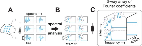
A three‐way spatio‐spectro‐epoch array of Fourier coefficients. To identify and characterize phase‐coupled oscillatory networks we obtain electrophysiological recordings from multiple sites and epochs, depicted schematically in A. We perform spectral analysis to describe oscillations at multiple frequencies, depicted in B. In the frequency domain, the average oscillatory activity in each epoch is described by a single complex‐valued Fourier coefficient per frequency. Fourier coefficients per site, frequency and epoch can be arranged in a three‐way array of Fourier coefficients, depicted in C. This three‐way array is the starting point for extracting phase‐coupled oscillatory networks. [Color figure can be viewed in the online issue, which is available at http://wileyonlinelibrary.com.]

The three‐way array of Fourier coefficients describes variation over sites, frequencies and epochs in the amplitudes and phases of oscillations generated in the underlying neural tissue. Phase consistency between sites in this three‐way array allows us to extract phase‐coupled oscillatory networks (Fig. 3). Because the three‐way array describes the average oscillatory activity in each epoch, these networks describe the average network activity in each epoch. We characterize a phase‐coupled oscillatory network using the following parameters: a frequency profile, a spatial amplitude map, a spatial time‐delay map (or frequency‐specific spatial phase maps), an epoch profile, and epoch‐specific phase offsets per frequency (Fig. 3B–G). All these parameters will be described below in detail. Importantly, this characterization follows from the assumption that oscillatory networks can be conceived as spatially distributed neuronal sources measured at a number of sites. The sources induce phase‐consistent oscillations measurable at different sites, within the frequencies that characterize the network. The phases of the frequency‐specific Fourier coefficients can vary both over sites and epochs but, because we assume phase‐consistency, the between‐site phase relations are identical for all epochs (Fig. 3A). Crucially, we characterize a network by multiple frequencies, which is in line with the general observation that neuronal oscillations always have energy in a band of frequencies. These frequencies can form a narrow range, for example, 4–8 Hz (the theta band), or a very broad range, for example, 30–60 Hz (the gamma band). Which frequencies are involved in a network is specified in the frequency profile.

Figure 3.

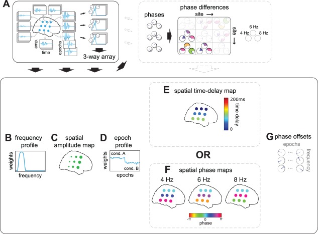
Phase‐coupled oscillatory networks describe spatially distributed patterns of phase coupling. A: Schematic of electrophysiological measurements reflecting a phase‐coupled oscillatory network. Phase‐coupled neuronal oscillations are measured at multiple sites, at multiple frequencies, and at multiple epochs. Measurements are arranged in a three‐way array of Fourier coefficients. Each column of sites in the grid displays underlying sources with increasing strength from left to right, and with increasing temporal delays from top to bottom. This delay results in frequency‐specific phase relations that increase with frequency, and with site row. Phase differences between sites are depicted in the phase differences diagram at 4, 6, and 8 Hz. Colors correspond to those in F. We define the network by a frequency profile (B), a spatial amplitude map (C), an epoch profile (D), a spatial time‐delay map (E), spatial phase maps (F), and phase offsets (G). B: frequency profile describing the average frequency band of the oscillations in A. C: spatial amplitude map describing the involvement of each site in the network. Circle size reflects the oscillatory amplitude in A. D: epoch profile describing the strength of the network in each epoch. The schematic network loads stronger in condition A than in B. E: spatial time‐delay map describing the temporal relation between sites producing the phase differences in A. Circle color reflects the relative time delay of each site, with respect to all other sites. This matches the time delay observable in the left‐hand side of A. F: frequency‐specific spatial phase maps describing the phase differences in A. Circle color reflects the relative phase of each site, and matches the first row of the diagram in A. From the spatial phase maps, all frequency‐specific phase differences can be reconstructed. G: Phase offsets capture frequency‐ and epoch‐specific phase offsets resulting from epoch‐specific temporal offsets. Note, as these phase offsets are not of interest when characterizing phase‐coupled oscillatory networks, they are shown in gray. [Color figure can be viewed in the online issue, which is available at http://wileyonlinelibrary.com.]

A frequency profile (Fig. 3B) specifies the degree to which different frequencies are involved in the network. It is described by a vector of positive real numbers, which are high for frequencies that are strongly involved, and close to zero for those that are weakly involved. A spatial amplitude map (Fig. 3C) specifies the degree to which the different sites reflect the network, and is also described by a vector of positive real numbers. An epoch profile (Fig. 3D) specifies the degree to which the different epochs reflect the network, also described by a vector of positive real numbers. The frequency profile, the spatial amplitude map, and the epoch profile (Fig. 3B–D) together describe the degree to which the network is determined by each of the 3 dimensions of the three‐way array of Fourier coefficients. All phase characteristics of the network are described by the spatial time‐delay map (Fig. 3E; or spatial phase maps, Fig. 3F), and the phase offsets (Fig. 3G). The latter of these, the phase offsets (Fig. 3G), capture the temporal offset of the network within each epoch. These phase offsets are frequency‐specific. The spatial time‐delay map (Fig. 3E; or frequency‐specific spatial phase maps, Fig. 3F) specifies the consistent between‐site phase relations. Importantly, we present a model for coupled oscillatory networks in which any two interacting sites is characterized by phase differences that may vary as a function of frequency (within the frequency band that characterizes this network). The way these phase differences vary over frequencies can provide important insights into how two sites interact. For instance, if there would be a consistent time delay between two interacting sites, then this would result in phase differences that increase linearly with frequency. These phase differences are jointly characterized by the spatial time‐delay map (Fig. 3E). A spatial time‐delay map is the map from which the time delay between any pair of sites can be obtained by taking the difference between the corresponding coefficients in the map. By multiplying this time delay with the frequency of interest, we obtain the between‐site phase difference for that frequency. The spatial phase maps (Fig. 3F) specify the between‐site phase differences more directly, without the constraint of a linear relation with frequency. These maps are frequency‐specific spatial maps from which the consistent between‐site phase differences can be obtained by simple subtraction between the sites. Because the spatial phase maps do not enforce a particular pattern on the between‐site phase differences (e.g., a linear relation with frequency), they are most useful in explorative studies. The spatial time‐delay maps are more useful for a targeted investigation of temporal dynamics. Importantly, although phase coupling at the level of site pairs can be reconstructed from both types of spatial maps, the maps themselves describe phase coupling at the level of individual sites. This is useful, because it can directly reveal the spatial structure of the network.

Together, the frequency profile, the spatial amplitude map, the epoch profile, the spatial time‐delay maps or spatial phase maps, and the phase offsets, characterize a phase‐coupled oscillatory network. That is, they describe that part of the three‐way array of Fourier coefficients that originates from a particular phase‐coupled oscillatory network. To extract and characterize these networks, we developed a new method, denoted as SPACE. This method is briefly described in the Materials and Methods Section, and a full description of the method and the underlying algorithm is provided in the Appendix. The method is based on two models: the time delay model (SPACE‐time) that characterizes networks using spatial time‐delay maps, and the FSP model (SPACE‐FSP), that characterizes networks using spatial phase maps. In the following, we first describe example networks extracted from ECoG recordings. Next, we provide evidence for the robustness of the method, by recovering simulated networks from realistic noisy data. In each section, both models are used and their results compared.

SPACE Extracts Phase‐Coupled Oscillatory Networks from Human ECoG Recordings

We now present three example networks extracted from ECoG recordings of three epilepsy patients while they were performing a Sternberg working memory task (see Materials and Methods; Fig. 4). We analyzed the task period during which the patients were engaged in the task. We did not distinguish between the cognitive operations encoding and retrieval occurring in this period, as the main purpose of the current analyses was to demonstrate that plausible phase‐coupled oscillatory networks could be extracted.

Figure 4.

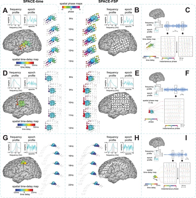
Example phase‐coupled oscillatory networks from human ECoG recordings. We show three‐phase‐coupled oscillatory networks from ECoG recordings during a Sternberg working memory task from three epilepsy patients (see Materials and Methods). Networks are displayed on a Talairach template brain. The first network shows a travelling alpha wave over parieto‐temporal electrodes (A,B,C). The second network shows an alpha network with phase relations dominated by 0 or $\pi$ over fronto‐parietal electrodes (D,E,F). The third network shows a travelling beta wave over parieto‐frontal electrodes (G,H,I). Each dataset was analyzed using the cross‐product formulation of SPACE‐time (A,D,G) and SPACE‐FSP (B,E,F) and the extracted networks were compared (see Materials and Methods). The Fourier coefficients were obtained from Welch‐tapered signals of 2 s, and therefore had a frequency resolution of 0.5 Hz. We also show single trial observations of the networks (C,F,I). Only those grids/strips with high amplitudes in the spatial amplitude map are shown. A: Travelling alpha wave described by the time delay model. Frequency and epoch profiles are shown in the top left. The full grid is shown in the center on a Talairach template. The spatial time‐delay map is shown on the right side. Electrode size reflects the spatial amplitude map. Electrode color reflects the time delay relative to the strongest electrode. The displayed frequencies are selected from the gray band in the frequency profile. Spatial phase maps are shown on the left to compare phases resulting from the time delay model to those of the FSP model. These maps were generated by multiplying each time delay by $2\pi {\phi }_k$, where ${\phi }_k$ reflects the $k$‐th frequency. B: Travelling alpha wave corresponding to the one in A described by the FSP model. Frequency and epoch profiles are shown on the top left. The spatial phase maps are displayed in the center. Electrode size reflects the spatial amplitude map. Electrode color reflects the phase relative to the strongest electrode in A. C: Single trial oscillations displaying the travelling alpha wave at the peak frequency (≈11 Hz) in the strongest trial. The top panel displays the selected trial, frequency, and electrodes. The bottom panel shows excerpts from this trial. Instantaneous amplitude is colored by instantaneous phase. The gray solid line reflects the time delay between electrodes. Oscillations matching the time delays cross this gray line at their peaks. Black arrows denote the direction of the travelling wave. D,E: same as A,B but for a dipolar alpha network with 0 or $\pi$ phase relations. F: same as in C but for the dipolar alpha network shown in D and E (≈11 Hz), using the estimates for the FSP model. The dashed gray line is now straight. Oscillations matching the spatial phase maps cross this line at their troughs for the top three electrodes and at their peaks for the bottom three electrodes. G,H: same as A,B but now for a travelling beta wave. I: same as C but now for the travelling beta wave (≈19 Hz) shown in G and H. [Color figure can be viewed in the online issue, which is available at http://wileyonlinelibrary.com.]

Fourier coefficients of each of the three datasets were obtained using a Welch tapering approach with multiple overlapping 2 second windows per trial, yielding a four‐way array of Fourier coefficients with a 0.5 Hz frequency resolution and a taper dimension (in contrast to the three‐way array introduced above, see Materials and Methods). Each of the three datasets was analyzed using both SPACE‐time and SPACE‐FSP. Because the four‐way arrays of Fourier coefficients were obtained using multitaper estimation, we used the cross‐product formulation of both models (see Materials and Methods and Appendix). Because we wanted to estimate the number of networks using a high frequency resolution (0.5 Hz), each epoch was constructed by combining the tapers of three consecutive trials (see Materials and Methods). The number of extracted networks was determined on the basis of their reliability as evaluated by a split‐half procedure (see Materials and Methods). This involves that only networks were extracted that could be identified in two independent datasets, obtained by randomly splitting the trials in two halves. This resulted in four, two, and four extracted networks from the recordings of patient 1, 2, and 3, respectively. We selected one network of each patient and show its description by the time delay and the FSP model (Fig. 4), all other networks are presented in Supporting Information Figs. S2–S4. We quantitatively compare both descriptions by a similarity coefficient (see Materials and Methods), which ranges from 0 to 1. The networks shown were selected because they reflect neurophysiologically interesting patterns, such as travelling waves. The three, one, and three non‐selected networks showed many different patterns, such as spatial amplitude/phase maps dominated by a few electrodes with little phase diversity and spatial amplitude/phase maps with multiple groups of electrodes exhibiting phase diversity both within and between groups.

From patient 1, we extracted a network that shows a travelling alpha wave over parieto‐temporal electrodes (Fig. 4A–C). The network extracted using the time delay model (Fig. 4A) closely corresponds to the one extracted using the FSP model (Fig. 4B): (1) the frequency profile and the epoch profile of the two networks are very similar (similarity coefficient = 0.91) and (2) the progression of phases over electrodes and over frequencies generated from the time delay network follows the spatial phase maps of the FSP network, with the time delay and the FSP network both showing the alpha wave travelling in the posterior to anterior direction. The only clear difference is that the spatial amplitude map of the FSP network includes more electrodes than the one of the time delay network. We also show the travelling wave in the trial with the highest amplitude at the peak frequency of the network (≈11 Hz). We do this for a selection of electrodes that lie in the direction of the travelling wave (Fig. 4C). This example shows that, at the level of a single trial, there is a close match between the time delays extracted using the time delay model (calculated over all trials) and these single trial time delays. We additionally computed the speed of the travelling wave using the network from the time delay model. This was done by computing the distances between all electrode‐pairs (using Talairach coordinates), dividing these distances by the between‐electrode time delays, and subsequently averaging the resulting speeds. (We calculated a weighted average with the weights being the product of the spatial amplitude map loadings of all electrode‐pairs.) This resulted in an average speed over electrode‐pairs for this travelling alpha wave of 4.38 m/s. This is similar to speeds reported by Massimini et al. [2004] in extracranial human recordings, but is much faster than those reported by Rubino et al. [2006] in ECoG recordings of monkey motor cortex. The direction of the wave is given by the temporal order of the time delays, provided that none of the between‐site time differences exceeds 2 s (a critical time delay that depends on the frequency resolution, which is 0.5 Hz for our analysis; see Appendix).

From patient 2, we extracted a dipolar alpha network over fronto‐parietal electrodes of which the spatial phase maps are dominated by phase relations that are either 0 or $\pi$ (Fig. 4D–F). The network extracted using the time delay model (Fig. 4D) closely corresponds to the one extracted using the FSP model (Fig. 4E; similarity coefficient = 0.96), except for the spatial time‐delay maps. The phase differences that are implied by the spatial time‐delay maps are much smaller than the phase relations that were estimated under the FSP model. We also show phase relations in the trial with the highest amplitude at the peak frequency of the network (≈11 Hz) for a selection of electrodes from the two clusters (Fig. 4F). The single trial phase differences between the two clusters of electrodes closely match the dipolar phase relations estimated under the FSP model.

From patient 3, we extracted a network that shows a travelling beta wave over fronto‐parietal electrodes (Fig. 4G–I). For all parameters, the network extracted using the time delay model (Fig. 4G) closely corresponds to the one extracted using the FSP model (Fig. 4H; similarity coefficient = 0.99). Importantly, the progression of phases over electrodes and over frequencies generated from the time delay network follows the spatial phase maps of the FSP network, with the time delay and the FSP network both showing the beta wave travelling in the anterior to posterior direction. We also show the phase relations in the trial with the highest amplitude at the peak frequency (≈19 Hz) for a selection of electrodes that lie in the direction of the travelling wave (Fig. 4I). The average speed over electrode‐pairs of this travelling beta wave was 5.19 m/s.

SPACE Recovers Phase‐Coupled Oscillatory Networks from Realistic Noisy Signals

We performed simulations to test the ability of our method to recover phase‐coupled networks from noisy signals. To accurately recover simulated networks, our method needs to fulfill two important requirements: (1) its solutions need to be unique and (2) it needs to be robust against biologically realistic noise. Although we cannot provide a theoretical proof of uniqueness, in the Appendix, we show the results of a simulation study that strongly suggest uniqueness. To investigate the second requirement, we conducted simulations using realistic noisy signals. These signals were obtained by adding spatially correlated noise to time‐domain signals that were generated under the time delay model. This spatially correlated noise reflects scattered neuronal sources without a consistent oscillatory phase coupling structure in some frequency range. These scattered sources distort the structure that is induced by the simulated networks because they cannot be fitted parsimoniously by our models. By increasing noise strength and spatial correlation, we create an environment where it becomes increasingly difficult to distinguish the networks of interest from the background activity. The importance of spatial correlation of the noise became very obvious when we performed pilot simulation studies with uncorrelated noise. We observed that it was trivially easy to accurately and uniquely recover networks in this situation. For instance, we simulated data in the frequency domain by directly generating the three‐way (and four‐way) array of Fourier coefficients using the parameters of both models. Adding large amounts of uncorrelated complex‐valued noise had a very weak effect on the recovery of the networks. To test our method under more challenging and more realistic conditions, we generated data in which we controlled both the amount and the spatial correlation of the noise.

We simulated phase‐coupled oscillatory networks with varying noise strength, spatial noise correlation, and time delays across a 5 × 5 sites grid (Figs. 5, 6, 7; for a detailed description see Materials and Methods). Using these simulations, we investigated (1) how network recovery varies as a function of noise strength and correlation and (2) how recovery varies as a function of the time delays. To this end we performed two sets of simulations: (1) fixed between‐site time delays but varying noise strength and spatial noise correlation and (2) varying time delays, varying noise strength but fixed spatial noise correlation. The SNR was varied over 4 levels: 4, 0.16, 0.04, and 0.01. Spatial noise correlation was determined by the FWHM of a bivariate Gaussian distribution at 0, 10, 20, or 40 mm. These distances are evaluated relative to the inter‐site distances of our 5 × 5 grid, which had a 10mm spacing. Finally, between‐site time delays were varied over the following 4 levels: 5, 25, 50, and 100 ms. In the following, we first briefly describe how we simulated phase‐coupled oscillatory networks, and how we assessed the similarity between the extracted and simulated networks. Next, we present the results of the two parts of our simulation study.

Figure 5.

Simulation of phase‐coupled oscillatory networks in a realistic noisy environment. To show that SPACE is able to recover networks surrounded by noise, we simulated a theta, alpha, and beta phase‐coupled oscillatory network on a 5 × 5 site grid with variable noise strength and spatial correlation (see Materials and Methods). Each network consisted of an oscillatory signal that progressed over sites with a time delay in a fixed order, and with partially overlapping sites. Signals were generated in three frequency bands, theta (4–8), alpha (8–12), and beta (10–25), and were present in 15 out of 25 epochs of 3 s. Each signal was constructed as band‐passed randomly generated brown noise per epoch, and lasted 1–1.5 s. Randomly generated brown noise was added to the signal. Both signal and noise had a 1/f ² shaped power spectrum. A: 5 × 5 site grid with 10 mm spacing showing simulated network progression and spatial correlation profile. The spatial amplitude maps had equal nonzero values for a subset of the sites. Amount of spatial correlation (right‐hand side of grid) was determined by a bivariate Gaussian with a FWHM of 0, 10, 20, and 40 mm. B: Frequency profile and epoch profile of simulated networks showing partial overlap. The frequency profile shows the average amplitude spectrum (shaded area = std‐dev) over epochs, over simulations. Colors indicate network identity and correspond to those in A. C: example epochs at various noise levels of a site displaying the theta network. [Color figure can be viewed in the online issue, which is available at http://wileyonlinelibrary.com.]

Figure 6.

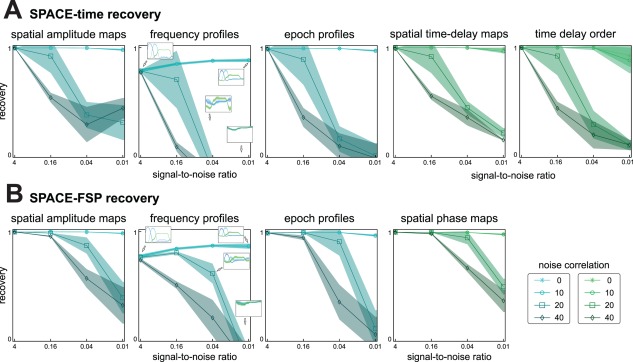
SPACE recovers simulated networks under noisy conditions. To investigate the effect of noise on the recovery of the simulated networks, we simulated networks with 25 ms time delay between adjacent sites, with variable noise strength, and spatial noise correlation (see Materials and Methods). SNR was systematically varied over 4, 0.16, 0.04, and 0.01. Spatial noise correlation was determined by a Gaussian with a FWHM at 0, 10, 20, or 40mm. For each combination of simulation parameters, we simulated 100 data sets. Each simulated data set was analyzed using the cross‐product formulation of SPACE‐time and SPACE‐FSP. The Fourier coefficients were obtained from Welch‐tapered signals of 1 s, and using additional Slepian tapering had a frequency resolution of 1 or 2 Hz (see Materials and Methods). We computed several coefficients reflecting the accuracy of recovery of the simulated networks. These range from −1 to 1 for spatial amplitude maps, frequency profiles, and epoch profiles. For spatial phase maps and spatial time‐delay maps, these range from 0 to 1. We additionally analyzed recovery of temporal order of time delays, with a coefficient ranging from 0 to 1. All coefficients were averaged over the three networks, per run. A: Average (over runs) recovery coefficients for SPACE‐time. Shading indicates standard‐deviation. Inserts in frequency profiles show the average extracted frequency profile. B: Same as in A but for SPACE‐FSP. A,B: the graphs show that (1) recovery is very accurate when noise is uncorrelated even when noise strength is high, (2) recovery decreases with noise correlation, (3) this decrease is stronger with higher noise strength, and (4) overall, SPACE‐FSP performs better than SPACE‐time. Note: the recovery of the frequency profiles does not approach a perfect fit. This is because we obtained the frequency profile to‐be‐recovered from a frequency analysis of the simulated time domain signals (band‐pass filtered brown noise). [Color figure can be viewed in the online issue, which is available at http://wileyonlinelibrary.com.]

Figure 7.

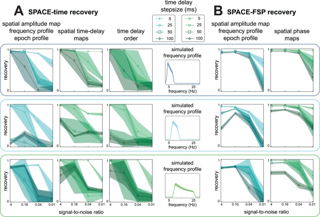
Recovery of simulated networks using SPACE for increasingly larger time delays between sites. To investigate the influence of time delay step size between adjacent sites on network recovery, we varied the time delay step size together with noise strength at a constant noise correlation (20 mm; see Materials and Methods. We simulated networks with 5, 25, 50, and 100 ms time delays between sites. SNR was set at 4, 0.16, 0.04, or 0.01. For each combination of simulation parameters, we simulated 100 data sets. Each simulated data set was analyzed using the cross‐product formulation of SPACE‐time and SPACE‐FSP. Fourier coefficients were calculated as in Figure 6. We quantified recovery using the same coefficients as in Figure 6. A: Average (over runs) recovery coefficients for SPACE‐time for the theta, alpha, and beta networks. Shading indicates standard deviation. An average recovery coefficient was computed per run over the spatial amplitude maps, frequency profiles, and epoch profiles. B: Same as in A but for SPACE‐FSP. We observe that (1) SPACE‐FSP is much less affected by the between‐site time delays than SPACE‐time, (2) goodness‐of‐recovery decreases with between‐site time delay and this decrease is much stronger for SPACE‐time, and (3) between‐site time delay and network frequency have interacting effects on goodness‐of‐recovery for SPACE‐time: with increasing time delay, goodness‐of‐recovery for the alpha network decreases more than for the theta and the beta network. [Color figure can be viewed in the online issue, which is available at http://wileyonlinelibrary.com.]

We simulated three‐phase coupled oscillatory networks travelling on a 5 × 5 sites grid, which were partially repeated over 25 epochs (Fig. 5). The three networks had different but partially overlapping frequency profiles: one in the theta, one in the alpha, and one in the beta band (Fig. 5B). Each network was further characterized by a spatial amplitude map specifying which sites showed the oscillatory signal and a spatial time‐delay map specifying the time and phase relations between these sites (Fig. 5A). Spatial amplitude maps were partially overlapping. Per network and epoch, a 1–1.5 s source signal was randomly generated as band‐pass filtered brown‐noise (see Materials and Methods), which was subsequently mapped to the sensor level (the 5 × 5 sites grid) according to the spatial amplitude and the spatial time‐delay map for that network. Per network, the frequency profile to‐be‐recovered was set as the average amplitude spectrum (over all epochs; Fig. 5B). Epochs varied with respect to whether or not a particular network was involved, and this was specified by the network's epoch profile (Fig. 5B). Each network was present in 15 out of 25 epochs. Noisy 3 second signals were created by adding randomly generated brown noise to the model signals that were generated as phase‐coupled oscillatory networks (after zero padding the 1–1.5 s model signals to 3 s). In Figure 5C, we show a set of example epochs with varying noise strength. For each of the simulation parameter combinations (4 SNR levels, four noise correlation levels and four time delays), we generated 100 data sets; each of these simulations will be denoted as a run. Per run, Fourier coefficients were obtained using a Welch tapering approach with multiple overlapping 1 second windows per epoch. This yielded a four‐way array of Fourier coefficients with a taper dimension and a 1 Hz frequency resolution for frequencies below 17 Hz and, using additional tapering, 2 Hz for frequencies of 17 Hz and above (see Materials and Methods). These four‐way arrays were subsequently analyzed using both SPACE‐time and SPACE‐FSP. Because the four‐way arrays of Fourier coefficients were obtained using multitaper estimation, we used the cross‐product formulation of both models. We computed recovery coefficients, expressing how well the extracted FSP and time delay model parameters recovered the simulated values (see Materials and Methods). These coefficients were computed per network per run. For the spatial amplitude maps, the frequency profiles, and the epoch profile of SPACE‐time/FSP, this coefficient ranges from −1 to 1. For the spatial phase maps and the spatial time‐delay maps, this coefficient ranges from 0 to 1. The recovery of the temporal order of the time delays (i.e., disregarding the quantitative differences) extracted by the time delay model was indexed by a coefficient that ranges from 0 to 1.

To investigate the effect of noise on the recovery of the networks, we simulated networks with a 25 ms time delay between adjacent sites and varying levels of noise strength and noise correlation (Fig. 6). This 25 ms time delay resulted in a delay of 125, 225, and 225 ms between the first and the last site for the theta, alpha, and the beta network, respectively. Recovery coefficients were calculated per network per run, and averaged over the three networks per run. Subsequently, the average and standard deviation over runs was calculated. We show these results, separately for SPACE‐time (Fig. 6A) and SPACE‐FSP (Fig. 6B). We observe that (1) without spatial noise correlation, recovery is highly accurate even for very high noise levels, (2) recovery decreases with noise strength, (3) this decrease is stronger with higher noise correlation, and (4) overall, SPACE‐FSP model performs better than SPACE‐time. To also give a visual impression of the goodness‐of‐recovery, we show the extracted frequency profiles for different levels of noise strength and noise correlation (Fig. 6A, B). Note that the recovery of the frequency profiles does not approach a perfect fit, both when using the time delay and the FSP model. This is because we obtained the frequency profile to‐be‐recovered indirectly by averaging the frequency spectra of the simulated time domain signals, instead of directly specifying the frequency profile and inserting it in the model equation (formulated in the frequency domain). Therefore, when evaluating the goodness‐of‐recovery, we do cannot compare the estimated profiles to the ground truth.

On the basis of these simulation results, we can formulate some guidelines for applications of SPACE to real data. For that, we consider a goodness‐of‐recovery coefficient of 0.75 to be sufficient for the label acceptable. Then, for an acceptable network recovery using the FSP model, it is sufficient to have an SNR of 0.16. The spatial noise correlation can then correspond to a noise FWHM covering 9 recording sites (i.e., 40 mm FWHM in the above). If the SNR is only 0.04, an acceptable network recovery requires that the noise FWHM covers at most 5 recording sites (a 20 mm FWHM in the above). For an acceptable network recovery using the time delay model, the spatial noise correlation has to be less: with an SNR of 0.16 or 0.04, the noise FWHM must cover at most 5 or 3 recording sites, respectively.

To investigate the effect of the between‐site time delays on network recovery, we varied the time delay step size together with noise strength at a fixed spatial noise correlation (20 mm FWHM). We simulated networks with a 5, 25, 50, and 100 ms delay between adjacent sites (Fig. 7. In this simulation study, we did not average the recovery coefficients over networks, as the frequency content of the different networks could have an influence on the ability to extract them. We show the recovery results for SPACE‐time (Fig. 7A) and SPACE‐FSP (Fig. 7B), separately for every network. For the purpose of presentation, we averaged the recovery coefficients for the spatial amplitude map, the frequency profile, and the epoch profile, and did this for each network in each run. We observe that (1) SPACE‐FSP is much less affected by the between‐site time delays than SPACE‐time, (2) goodness‐of‐recovery decreases with between‐site time delay and this decrease is much stronger when using the time delay model, and (3) between‐site time delay and network frequency have interacting effects on goodness‐of‐recovery when using the time delay model: with increasing time delays, goodness‐of‐recovery for the alpha network decreases more than for the theta and the beta network. We therefore conclude that, when expected time delays are large, using the FSP model is preferred over the time delay model.

In sum, we have shown that SPACE can recover networks from signals that contain spatially correlated noise. For the FSP model, an SNR of 0.16 suffices to produce an acceptable recovery even when the spatial noise correlation encompasses 9 recording sites. If the SNR is only 0.04, an acceptable network recovery requires that the spatial noise correlation encompasses at most five recording sites. For an acceptable network recovery using the time delay model, the spatial noise correlation has to be substantially less. Additionally, when the expected time delays of a phase‐coupled oscillatory network are large relative to cycle length of the network oscillation, then SPACE‐FSP can more accurately recover the between‐site phase relations generated from the time delays.

DISCUSSION

We developed a method capable of extracting phase‐coupled oscillatory networks. Our contribution involves four‐key elements. First, we provide a precise definition of a phase‐coupled oscillatory network in terms of six parameters: a frequency profile, a spatial amplitude map, spatial phase maps or a spatial time‐delay map, an epoch profile, and phase offsets (or an equivalent parameter in case of the cross‐product formulation). Crucially, this definition respects the fact that brain rhythms involve a range of frequencies, and cannot be characterized by line spectra. Second, we developed a method that extracts these networks from electrophysiological data. Third, we demonstrate that this method is able to extract networks with a revealing phase structure from ECoG data. And fourth, using a simulation study, we quantify the robustness of this method against violations of the phase‐coupling structure imposed by the model. This demonstrates the method's usefulness in practical applications.

Neuronal networks realize the many processes that underlie cognitive functions: selecting and routing information, keeping the information in working memory, storing and retrieving information from a more permanent store, and so forth. All these processes involve interactions between anatomically distinct but connected brain regions. This is the prime motivation for the development of methods that extract these networks from neurobiological data.

Compared to electrophysiology, the fMRI community has a long tradition in identifying functional networks. Networks of coactivated brain regions can be found using the spontaneous covariation of the blood oxygenation level dependent signal measured at rest, that is, in absence of stimulation or a task [Biswal et al., 1997; Deco and Corbetta, 2011; Fox et al., 2005; Honey et al., 2009; Raichle et al., 2001; Smith et al., 2009]. These networks are usually referred to as resting state networks [RSNs; Beckmann et al., 2005]. An important observation constraining the possible functional role of these fMRI‐derived RSNs is that they also exist in the absence of consciousness during anesthesia and sleep [Vincent et al., 2007].

Recently, RSNs have begun to be investigated using magnetoencephalography (MEG) recordings [Brookes et al., 2011; de Pasquale et al., 2010]. This is important progress, because MEG directly measures electrophysiological brain activity, bypassing the indirect hemodynamic response. Crucially, the RSNs that were identified did not depend on oscillatory phase coupling. As a part of the analyses, MEG recordings were transformed into time series of band‐limited power (BLP) in several frequency bands. These BLP time series were then correlated using a seed‐based approach [de Pasquale et al., 2010] or decomposed using independent component analysis [Brookes et al., 2011]. With this approach, it was shown that RSNs could be extracted using BLP time series (especially in the beta band; 15–25 Hz) that were highly similar to those found in fMRI signals [Brookes et al., 2011; de Pasquale et al., 2010].

Another recent method to identify networks is based on phase‐amplitude coupling [Maris et al., 2011; van der Meij et al., 2012]. Contrary to a correlation between BLP time series, phase‐amplitude coupling does depend on oscillatory phase coupling: it indexes the preference for amplitude envelopes at a certain frequency (equivalent to a BLP time series) to have high values at a certain phase of a slower phase‐providing oscillation. Most reports focus on the coupling between amplitude‐providing and phase‐providing oscillations obtained from the same site [Bruns and Eckhorn, 2004; Canolty et al., 2006; Chrobak and Buzsaki, 1998; Cohen et al., 2009; Mormann et al., 2005; Schack et al., 2002]. However, focusing on between‐site phase‐amplitude coupling inspired the development of methods with which networks could be identified [Maris et al., 2011; van der Meij et al., 2012]. With these methods, revealing differences between amplitude‐providing and phase‐providing networks could be identified.

The method presented in this article allows for an identification of networks using phase coupling between oscillations alone. Crucially, this method respects the fact that brain rhythms have energy in a range of frequencies, and therefore allows between‐site phase differences to vary over frequencies. As we have illustrated in the Results Section, this property allows us to distinguish different network configurations. One such example is a travelling wave (e.g., the networks in Fig. 4A, G, and the simulated networks in Figs. 5−7). This wave could be generated by a distributed oscillatory source in which the many subpopulations interact with a temporal delay. The signals generated by such a distributed source can be described by our time delay model. A second example, which can be described by our FSP model, involves a source that is small relative to its distance from the sensors, as is often the case in macroscopic measurements like MEG and electroencephalography (EEG), but is also present in more local measurements such as ECoG (see Results Section). Such a distant source generates a dipolar potential distribution (two groups of sites whose potentials have opposite signs) over sites that are at the same distance from this source (e.g., the network in Fig. 4E, network 2 in Fig. S2B, and network 1 Fig. S3B). The phase differences between these sites are either 0 (synchrony) or $\pi$ (antiphase) and, importantly, do not vary as a function of frequency. This example shows that the spatial phase maps can depend on the recording technique. The dependence of the spatial distribution of the measurements on the recording technique has been put forward by other authors, starting from the spatial filtering characteristics of the measurement technique [Nunez et al., 2001]. A third example is a network driven by thalamocortical interactions [Suffczynski et al., 2001], which has elements of the above two examples. A possible scenario involves multiple cortical populations that are driven by a common thalamic pacemaker. The timing of the input to these cortical populations will differ as a function of the delay in the axonal connection with this thalamic pacemaker. As a result, the phase relations between these cortical populations will be larger than the phase relations within them (which are 0 in the idealized scenario of no within‐population differences in axonal delay). The essential difference with this example configuration and the previous dipolar configuration is that between‐site phase differences are not only 0 or $\pi$, but can take any value in between (as determined by the difference in thalamocortical delay). Such a network can be described by both of our models.

Between‐site phase relations in electrophysiological recordings may be of crucial importance for the understanding of neuronal communication. Electrophysiological recordings of neural activity (local field potentials (LFPs), ECoG, EEG, MEG) reflect synchronized membrane potential fluctuations. Importantly, membrane potential fluctuations reflect fluctuations in neuronal excitability. This implies that oscillations may reflect rhythmic fluctuations in neuronal excitability. It has therefore been proposed that effective communication between two neuronal populations depends on whether or not the spike input from the sending population arrives at an excitable phase of the receiving population [Borgers and Kopell, 2008; Fries, 2005; Tiesinga et al., 2008]. This idea can easily be generalized to motifs that involve more than two neuronal populations, of which some pairs can effectively communicate and others cannot, depending on their phase relations [Fries, 2005]. Thus, neuronal populations forming networks by phase‐coupled oscillations could be a key mechanism for interareal communication and selective routing of information through the brain. In line with this hypothesis, it has been shown that local field potentials at one site coordinate spikes in task‐relevant neurons at a remote site [Canolty et al., 2010, 2012b].

From a methodological point of view, it is important to distinguish our multivariate approach from the more common bivariate approach, in which oscillatory phase coupling is evaluated by pair‐wise measures such as coherence [Mormann et al., 2000], imaginary coherence [Nolte et al., 2004], phase‐locking value [Lachaux et al., 1999], pair‐wise phase consistency [Vinck et al., 2010], the phase‐slope index [Nolte et al., 2008], and Granger causality [Bernasconi and Konig, 1999; Kaminski et al., 2001]. Some methods can make use of a full multivariate description of the data, but nevertheless only provide a quantification at the level of site‐pairs, using the multivariate description to partial out for the contribution of other sites. This holds for phase coupling estimation [Canolty et al., 2012a], partial coherence [Rosenberg et al., 1998], Granger causality [Bernasconi and Konig, 1999; Kaminski et al., 2001], Transfer Entropy [Schreiber, 2000], and Phase Transfer Entropy [Lobier et al., 2014]. This quantification at the level of site‐pairs is unfortunate, as pair‐wise measures do not directly reveal the spatial distribution of phase‐coupled networks, unless there is prior information about a seed region via which the other nodes of the network can be identified.

A method that shares several aspects with the method presented in this article is shifted CP [SCP; Morup, et al., 2008]. This method builds on earlier work in which PARAFAC [Carrol and Chang, 1970; Harshman, 1970] was used to decompose spatio‐spectro‐temporal electrophysiological data [Miwakeichi et al., 2004; Morup et al., 2006]. Importantly, in these earlier studies, PARAFAC was only applied to the amplitudes of the Fourier coefficients; the phase information was ignored. The novel method, SCP, decomposes the complex‐valued raw Fourier coefficients over sites, frequencies and epochs into multiple components. Each SCP component is described by a real‐valued spatial map, a complex‐valued frequency profile, and a real‐valued epoch profile. Importantly, each component is additionally described by a set of epoch‐specific time‐shifts, which allows the method to model between‐epoch differences in the temporal onset of a network. However, as between‐site phase relations are not explicitly modeled, only networks with between‐site phase differences of 0 and $\pm \pi$ are extracted (by allowing for negative values in the spatial maps). Though this makes SCP suitable for extracting dipolar potential distributions, other types of phase‐coupled oscillatory networks cannot be accurately described.

What holds for the comparison with shifted CP, also holds for the comparison with other decompositions, such as independent component analysis (ICA) [Bell and Sejnowski, 1995] and regular PARAFAC for complex‐valued data [Sidiropoulos et al., 2000]: our method improves on these alternatives because it is grounded in a plausible model of a neurobiological rhythm, a spatially distributed signal with energy in a limited range of frequencies and involving between‐site phase relations that vary as a function of frequency. For example, we could apply complex‐valued PARAFAC to a three‐way array of raw Fourier coefficients obtained from electrophysiological data. To our knowledge, this has not been reported yet, but there is nothing that prevents it. However, when applying this model, it imposes the restriction that the between‐site phase relations in a network are identical for all frequencies. In contrast, our method extracts phase‐coupled oscillatory networks that are characterized by a single spatial amplitude map and multiple frequency‐specific spatial phase maps, as is required for modeling brain rhythms whose between‐site phase relations depend on frequency.

Our method estimates spatial maps and frequency profiles without applying constraints on the shape of the spatial or spectral distribution. This is not necessarily optimal, and future improvement of our method could involve such constraints. Especially smoothness constraints could turn out to be beneficial, and improve the interpretability of the extracted spatial structure and spectral content of networks. Such constraints have been applied successfully before in source reconstruction methods, such as LORETA [Pascualmarqui et al., 1994].

It is useful to compare our approach to the more theory‐driven approach of computational neuroscientists that build networks of spiking model neurons, often with the objective of explaining correlated neuronal activity [e.g., Borgers and Kopell, 2003; Kopell et al., 2000; Whittington et al., 2000]. These networks of spiking model neurons serve as the neurobiological motivation for network models at a coarser level of description, typically involving weakly coupled Kuramoto oscillators [Brown et al., 2004; Ermentrout and Kopell, 1990; Hoppensteadt and Izhikevich, 1997; Kuramoto, 1984, 1997]. Networks of Kuramoto oscillators are characterized by their phase interaction function (PIF), which specifies how the oscillators affect each other's phase velocity. These networks describe dynamics in phase relations and therefore can be used to model non‐stationary processes. SPACE can also be applied to non‐stationary processes, but can accommodate non‐stationarity only by adding networks, because every network can only model a stationary pattern of phase relations.

Ideally, we would be able to motivate our method by establishing the relation between the parameters of the uncovered networks and a set of PIFs that may underlie these parameters. This would ground the output of our method in the well‐developed mathematical theory of Kuramoto models. Unfortunately, it is unclear what the relation is between, on the one hand, the phase configurations induced by a Kuramoto model (e.g., different types of travelling waves), and on the other hand, Fourier coefficients (the raw frequency domain observations when actual data are collected). This state of affairs limits the application of Kuramoto models to a comparison between observed and simulated/fitted phase configurations, as is possible for instance using Bayesian model comparison [see Penny et al., 2009, for an example of this approach]. This differs from our approach in which we estimate the full networks from the raw Fourier coefficients.

In conclusion, our work starts from a precise definition of a phase‐coupled oscillatory network that is in agreement with the fact that brain rhythms have energy in a range of frequencies. Crucially, this definition and the associated method allow for between‐site phase relations that vary as a function of frequency. This allows us to distinguish different network configurations. Our method identifies networks on the basis of between‐site phase coupling. This is an important contribution because (1) the existing bivariate methods can only indirectly reveal networks (using a seed region approach) and (2) the existing multivariate methods can only identify networks using amplitude envelope correlations. When identifying networks of oscillatory brain activity, it is crucial to take into account between‐site phase relations. Because oscillations may reflect rhythmic fluctuations in neuronal excitability, phase‐coupled oscillatory networks could be the functional building block for inter‐areal communication and selective routing of information throughout the brain.

Supporting information

Supporting Information

Supporting Information

Supporting Information

Supporting Information

Supporting Information

SPACE: An Alternating Least Squares Algorithm for Extracting Phase‐Coupled Oscillatory Networks

We developed a method for extracting phase‐coupled oscillatory networks from a three‐ or a four‐way array of Fourier coefficients. This algorithm is denoted as SPACE. It is inspired by complex‐valued PARAFAC [Bro, 1998; Carrol and Chang, 1970; Harshman, 1970; Sidiropoulos et al., 2000], an N‐way decomposition technique. PARAFAC describes the structure in an N‐way array by sets of loading vectors (one vector per dimension), which are jointly denoted as components. These components are extracted without requiring statistical constraints like orthogonality or independence, and are unique up to trivial indeterminacies. PARAFAC formed the base from which our new method was build, and it inherits many of its aspects.

SPACE uses two models to extract phase‐coupled networks, which are described below (see the Materials and Methods and Results Sections for a concise graphical introduction to the method). Extracting phase‐coupled oscillatory networks starts with electrophysiological measurements $V_{jl}\left(t\right)$ (electrical potentials or magnetic field strength) as a function of time $t$, at multiple sites $j$, and in multiple epochs $l$. Then, by performing a spectral analysis on $V_{jl}\left(t\right)$ we can describe the average (over the epoch) oscillatory activity at site $j$ and in epoch $l$ by a complex‐valued Fourier coefficient $X_{jkl}$, per frequency $k$. These Fourier coefficients can then be arranged in a three‐way array, with dimensions sites ( $J$), frequencies ( $K$), and epochs ( $L$). This three‐way array of Fourier coefficients is the starting point for our method to extract phase‐coupled oscillatory networks. These networks describe spatially distributed patterns of phase‐coupling, by a spatial amplitude map, a frequency profile, an epoch profile, a spatial phase map per frequency, and a set of phase offsets.

SPACE uses two models to extract networks: SPACE‐time and SPACE‐FSP, which differ in how they describe the between‐site phase relations per frequency. SPACE‐time describes all phase differences (which vary as a function of frequency) by site‐specific time delays, forming a spatial time‐delay map. SPACE‐FSP describes the between‐site phase differences by site‐ and FSP, forming a spatial phase map per frequency. Importantly, the phase differences at the level of the site‐pairs are calculated from the spatial time‐delay map and spatial phase maps (representations at the level of the sites, instead of site‐pairs). The element‐wise formulations of these two models are as follows:

$$\text{SPACE}-\text{time}: X_{jkl}= \sum _{f=1}^F{a}_{jf}\cdot \text{exp}\left(i2\pi {\phi }_k{\sigma }_{jf}\right)\cdot b_{kf}\cdot c_{lf}\cdot \text{exp}\left(i2\pi {\tau }_{klf}\right)+{\varepsilon }_{jkl}$$

$$\text{SPACE}-\text{FSP}: X_{jkl}= \sum _{f=1}^F{a}_{jf}\cdot \text{exp}\left(i2\pi {\lambda }_{jkf}\right)\cdot b_{kf}\cdot c_{lf}\cdot \text{exp}\left(i2\pi {\tau }_{klf}\right)+{\varepsilon }_{jkl}$$

The Fourier coefficient $X_{jkl}$ is described as a sum over $F$ network‐specific complex‐valued numbers. For both models, the amplitude of each network‐specific complex‐valued number is the product of $a_{jf}$, $b_{kf}$, and $c_{lf}$, which refer to, respectively, the spatial amplitude map, the frequency profile and the epoch profile. For the time delay model the phase of each network‐specific complex‐valued number is the product of an element of the spatial time‐delay map and a phase offset: $\text{exp}\left(i2\pi {\phi }_k{\sigma }_{jf}\right)$ and $\text{exp}\left(i2\pi {\tau }_{klf}\right)$. Here, $2\pi {\phi }_k{\sigma }_{jf}$ describes the site‐, frequency‐, and network‐specific phases, in which ${\phi }_k$ denotes the $k$‐th frequency (in Hz) and ${\sigma }_{jf}$ denotes the site‐ and frequency‐specific time delay. $2\pi {\tau }_{klf}$ describes the frequency‐, epoch‐, and network‐specific phase offset. For the FSP model, the phase of each network‐specific complex‐valued number is the product of an element of the spatial phase maps and a phase offset: $\text{exp}\left(i2\pi {\lambda }_{jkf}\right)$ and $\text{exp}\left(i2\pi {\tau }_{klf}\right)$. Compared to the time delay model, ${\phi }_k{\sigma }_{jf}$ is replaced by ${\lambda }_{jkf}$. Using the above parameterization of phase‐coupled oscillatory networks our model sparsely describes an array of $2JKL$ elements (with the 2 reflecting the complex‐valued nature of the input data) by sets of $2J+K+L+KL$ (SPACE‐time) or $J+JK+K+L+KL$ (SPACE‐FSP) elements.

All parameters are estimated using an ALS algorithm. Within each ALS iteration, we alternate over the five parameter sets characterizing the networks, obtaining a new LS estimate of each, while keeping the other four parameter sets fixed. After all parameters are updated, a single iteration is completed. This process continues until a predetermined convergence criterion is reached.

We now describe the calculations within a single ALS iteration. Whereas the estimation of the spatial amplitude maps, the frequency and the epoch profiles uses known equations, the estimation of the time delays, FSP, and phase offsets requires new algorithms, and these are described in a separate paragraph below.

All parameters are initialized by random starting values. Importantly, like PARAFAC, the algorithm can converge to a local minimum of the LSs loss function. These suboptimal decompositions can be avoided by starting the algorithm multiple times. When the algorithm repeatedly converges to the same optimal solution starting from multiple random starting points, it can be assumed that the global minimum is reached. Besides local minima, as a consequence of an unfortunate starting point, the algorithm may also get trapped in a degenerate solution, in which networks become highly correlated, and the model estimates become arbitrarily large. This is a well‐known problem in PARAFAC [see Bro, 1998, and the references therein] and can be dealt with using multiple random starts. Another strategy to avoid degeneracy is presented below in the section describing the cross‐product formulation of both models.

The algorithm(s) described below will be made available in a public GitHub (http://www.github.com) repository termed nwaydecomp. Additionally, it will be made available through the FieldTrip open‐source MATLAB toolbox [Oostenveld et al., 2011].

Obtaining the Least Squares Estimates of the Spatial Amplitude Maps, the Frequency and the Epoch Profiles

The LS estimation of the spatial amplitude maps ( $a_{jf}$), frequency profiles ( $b_{kf}$) and epoch profiles ( $c_{lf}$) resembles an ALS step in PARAFAC, however with two important differences. First, these maps and profiles are real‐valued parameters in a complex‐valued LSs minimization problem. As will be described in more detail in the next paragraph, this requires that the real and imaginary parts of some complex‐valued matrices are concatenated, resulting in an expanded real‐valued matrix. Second, we cannot make use of the regular Khatri–Rao product formulation, which plays a central role in the ALS algorithm for PARAFAC. This is due to the fact that the phases resulting from the time delays, the spatial phase maps and the epoch‐specific phase offsets are frequency‐specific. As a consequence, the LSs estimates of the spatial amplitude maps ( $a_{jf}$), frequency profiles ( $b_{kf}$), and epoch profiles ( $c_{lf}$) are obtained separately for every site, frequency, and epoch. We first describe the estimation of the spatial amplitude maps; the estimation of the frequency and the epoch profiles has exactly the same structure. The LSs estimate of the parameters of the $j$‐th site are obtained as follows:

$$A_j=X_j^{\text{cat}}\cdot Z^{\text{cat}}\cdot {\left(Z^{\text{cat}}{}^{{}^T}\cdot Z^{\text{cat}}\right)}^{-1}$$ (2)

$A_j$ is a vector of size $1\times F$, ${}^T$ denotes the regular transpose and ${}^{-1}$ denotes the inverse. Here, $Z^{\text{cat}}$ and $X_j^{\text{cat}}$ refer to $\left[\text{Real}\left(Z\right), \text{Imag}\left(Z\right)\right]$ and $\left[\text{Real}\left(X_j\right); \text{Imag}\left(X_j\right)\right]$, which are the row‐wise and column‐wise concatenation of the real and imaginary parts of $Z$ and $X_j$, respectively. Matrix $X_j$ is the unfolded matrix of Fourier coefficients for site $j$, with unfolding over the frequency and epoch dimensions. This results in a matrix with dimensions $1\times KL$ (with $K$ and $L$ being the number of frequencies and epochs, respectively). Matrix $Z$ is a complex‐valued matrix formed in two steps. In the first step, the amplitude of the elements of $Z$ are calculated, and in the second step, their phase. The amplitude of $Z$ is given by $C|\otimes |B$, the Khatri–Rao product of the epoch and frequency profiles, $C$ and $B$. The matrices $C$ and $B$ contain as their columns, respectively, the frequency and the epoch profiles of the different networks. The Khatri–Rao product $|\otimes |$ is defined as follows:

$$C|\otimes |B= \left[c_1\otimes b_1 c_2\otimes b_2 \dots c_F\otimes b_F\right]$$

This applies to any matrix $C$ and $B$ with an equal number of columns $F.$ The Kha tri‐Rao product is defined as the concatenation of the Kronecker tensor products $\otimes$ of column $1$ to $F$ of $C$ and $B$. The phases of the elements of $Z$ are calculated as element‐wise products of the spatial phase maps (for the time delay model obtained from the spatial time‐delay maps) and the phase offsets. These products are calculated in such a way that the indices of the frequencies and the epochs correspond to the amplitudes as calculated by the Khatri–Rao product.

The LSs estimate of the frequency and epoch profiles are calculated similarly to the spatial amplitude maps. For the frequency profile $X_j^{\text{cat}}$ is replaced by $X_k^{\text{cat}}$. $X$ is now a matrix unfolded over the site and epoch dimensions, having dimensions $1\times JL$ (with $J$ being the number of sites). The amplitude of matrix $Z$ is now calculated as $C|\otimes |A$, with $A$ containing in its columns the spatial amplitude maps. The phases of $Z$ are again calculated as a product of the phase parameters described above, with the indices corresponding to the Khatri‐Rao product. For the epoch profiles, $X_j^{\text{cat}}$ is replaced by $X_l^{\text{cat}}$, and the Khatri–Rao product for the amplitude of $Z$ by $B|\otimes |A$. The procedure for the phases of Z is adjusted accordingly.

Obtaining the Least Squares Estimates of Time Delays and Frequency‐Specific Phases

The time delays and FSP are estimated using a method that starts from a rewriting of the LS loss function as a sum of trigonometric functions. This sum can be minimized using a combination of a steepest descent and a modified Newton–Raphson algorithm. The entire procedure is described below for a three‐way array. It is straightforward to adjust this procedure to a four‐way array with a taper dimension.

First, the LS loss function is rewritten as a linear combination of trigonometric functions, with $\sigma$ or $\lambda$, and $\tau$ as parameters. We now show how this can be done:

$$\text{Loss}\hspace{0.17em}\text{function}\hspace{0.17em}\text{for}\hspace{0.17em}\sigma :{\left|\right|{\varepsilon }_{jkl}\left|\right|}^2={\left|\right|X_{jkl}-\sum _{f=1}^F{a}_{jf}\cdot b_{kf}\cdot c_{lf}\cdot \text{exp}\left(i2\pi {\phi }_k{\sigma }_{jf}+i2\pi {\tau }_{klf}\right)\left|\right|}^2$$

$$\text{Loss}\hspace{0.17em}\text{function}\hspace{0.17em}\text{for}\hspace{0.17em}\lambda :\hspace{0.17em}{\left|\right|{\varepsilon }_{jkl}\left|\right|}^2={\left|\right|X_{jkl}-\sum _{f=1}^F{a}_{jf}\cdot b_{kf}\cdot c_{lf}\cdot \text{exp}\left(i2\pi {\lambda }_{jkf}+i2\pi {\tau }_{klf}\right)\left|\right|}^2$$

Here, $\left|\right|\hspace{0.17em}\left|\right|$ denotes the norm. By substituting $2\pi {\phi }_k{\sigma }_{jf}$ with ${\Phi }_{jkf}$ and $2\pi {\lambda }_{jkf}$ with ${\Phi }_{jkf}$, both equations can be described jointly by:

$${\left|\right|{\varepsilon }_{jkl}\left|\right|}^2={\left|\right|Z_{jkl}\cdot \text{exp}\left(i{\Psi }_{jkl}\right)-\sum _{f=1}^F{\widehat{Z}}_{jklf}\cdot \text{exp}\left(i{\Phi }_{jkf}+i{T}_{klf}\right)\left|\right|}^2$$

where $T_{klf}$ denotes $2\pi {\tau }_{klf}$, ${\widehat{Z}}_{jklf}$ denotes $a_{jf}\cdot b_{kf}\cdot c_{lf}$, and $Z_{jkl}\cdot \text{exp}\left(i{\Psi }_{jkl}\right)$ denotes $X_{jkl}$. Then, using Euler's formula, and substituting ${\Phi }_{jkf}+T_{klf}$ with ${\widehat{\Psi }}_{jkl}$, this becomes:

$${\left|\right|{\varepsilon }_{jkl}\left|\right|}^2={\left|\right|\left(\left[Z_{jkl}\cdot \cos {\Psi }_{jkl}\right]-\sum _{f=1}^F\left[{\widehat{Z}}_{jklf}\cdot \cos {\widehat{\Psi }}_{jkl}\right]\right)+i\left(\left[Z_{jkl}\cdot \sin {\Psi }_{jkl}\right]-\sum _{f=1}^F\left[{\widehat{Z}}_{jklf}\cdot \sin {\widehat{\Psi }}_{jkl}\right]\right)\left|\right|}^2$$

Replacing the squared norm by a sum of squares, we get:

$${\left|\right|{\varepsilon }_{jkl}\left|\right|}^2={{\left(\left[Z_{jkl}\cdot \cos {\Psi }_{jkl}\right]-\sum _{f=1}^F\left[{\widehat{Z}}_{jklf}\cdot \cos {\widehat{\Psi }}_{jkl}\right]\right)}^2+\left(\left[Z_{jkl}\cdot \sin {\Psi }_{jkl}\right]-\sum _{f=1}^F\left[{\widehat{Z}}_{jklf}\cdot \text{sin}{\widehat{\Psi }}_{jkl}\right]\right)}^2$$

In the next step, we complete the square and simplify the resulting equation. Then, using the angle addition identity, the Pythagorean identity, replacing ${\widehat{\Psi }}_{jkl}$ by ${\Phi }_{jkf}+T_{klf}$, and using trigonometric symmetry, we get:

$${\left|\right|{\varepsilon }_{jkl}\left|\right|}^2=Z_{jkl}^2+{\widehat{Z}}_{jklf}^2+\sum _{f=1}^{F}2Z_{jkl}{\widehat{Z}}_{jklf}\cos \left({\Phi }_{jkf}+\left(T_{klf}-{\Psi }_{jkl}+\pi \right)\right)+\sum _{f=1}^{F-1}\sum _{n=f+1}^{F}2{\widehat{Z}}_{jklf}{\widehat{Z}}_{jkln}\cos \left({\Phi }_{jkf}-{\Phi }_{jkn}+\left(T_{klf}-T_{kln}\right)\right)$$

The least squared error of ${\Phi }_{jkf}$ is computed by summing over $k,l$. Applying the sum, and using the harmonic addition identity, the equation reaches its final form used for optimization:

$$\sum _{k=1}^K\sum _{l=1}^L{\left|\right|{\varepsilon }_{jkl}\left|\right|}^2={\alpha }_j+\sum _{k=1}^K\sum _{f=1}^F\left[{\beta }_{jkf}\text{cos}\left({\Phi }_{jkf}+{\zeta }_{jkf}\right)\right]+\sum _{k=1}^K\sum _{f=1}^{F-1}\sum _{n=f+1}^F\left[{\gamma }_{jkfn}\cos \left({\Phi }_{jkf}-{\Phi }_{jkn}+{\eta }_{jkfn}\right)\right]$$ (3)

The parts of the above equation are as follows:

$${\alpha }_j=\sum _{k=1}^K\sum _{l=1}^L\left[Z_{jkl}^2+\sum _{f=1}^F{\widehat{Z}}_{jklf}^2\right]$$

$${\beta }_{jkf}=\sqrt{{\left(\sum _{l=1}^{L}2Z_{jkl}{\widehat{Z}}_{jklf}\cos \left(T_{klf}-{\Psi }_{jkl}+\pi \right)\right)}^2+{\left(\sum _{l=1}^{L}2Z_{jkl}{\widehat{Z}}_{jklf}\sin \left(T_{klf}-{\Psi }_{jkl}+\pi \right)\right)}^2}$$

$${\zeta }_{jkf}=a\text{tan}2\left(\frac{{\sum }_{l=1}^{L}2Z_{jkl}{\widehat{Z}}_{jklf}\sin \left(T_{kln}-{\Psi }_{jkl}+\pi \right)}{{\sum }_{l=1}^{L}2Z_{jkl}{\widehat{Z}}_{jklf}\cos \left(T_{kln}-{\Psi }_{jkl}+\pi \right)}\right)$$

$${\gamma }_{jkfn}=\sqrt{{\left(\sum _{l=1}^{L}2{\widehat{Z}}_{jklf}{\widehat{Z}}_{jkln}\cos \left(T_{klf}-T_{kln}\right)\right)}^2+{\left(\sum _{l=1}^{L}2{\widehat{Z}}_{jklf}{\widehat{Z}}_{jkln}\sin \left(T_{kln}-T_{kln}\right)\right)}^2}$$

$${\eta }_{jkfn}=a\text{tan}2\left(\frac{{\sum }_{l=1}^{L}2{\widehat{Z}}_{jklf}{\widehat{Z}}_{jkln}\sin \left(T_{klf}-T_{kln}\right)}{{\sum }_{l=1}^{L}2{\widehat{Z}}_{jklf}{\widehat{Z}}_{jkln}\cos \left(T_{klf}-T_{kln}\right)}\right)$$

In the last equation, atan2 refers to the four‐quadrant arctangent and ${\Phi }_{jkf}$, denotes either $2\pi {\phi }_k{\sigma }_{jf}$ or $2\pi {\lambda }_{jkf}$.

By minimizing the function in Eq. (3) with respect to ${\sigma }_{jf}$ (time delay model) or ${\lambda }_{jkf}$ (FSP model) we obtain their LS estimates. We use different nonlinear optimization procedures for the FSP and the time delay model. For every site‐frequency pair ( $j,k$) in the FSP model, we perform an $F$‐dimensional minimization with respect to the ${\lambda }_{jkf}$ of all $F$ networks. First, we decrease the LS loss function by means of steepest descent until the Hessian matrix of this function becomes positive definite. Subsequently, we minimize the loss function using modified Newton–Raphson. The step size used in steepest‐descent and modified Newton–Raphson is determined such that the loss function decreases with every step.

For the time delay model, we perform a one‐dimensional minimization with respect to ${\sigma }_{jf}$ for every site‐network pair ( $j,k$). As for the FSP model, this minimization is performed using a combination of steepest descent and modified Newton–Raphson. Importantly, the loss function for the ${\sigma }_{jf}$ parameter is rhythmic, and contains many local minima. Therefore, to find the global minimum, an initial estimate has to be found which is in the same cycle that also contains the global minimum. This initial estimate is found by an informed sparse grid search. The sparse grid search is informed by the cycle length of the term in Eq. (3) with the highest frequency, which is the term with the fastest rhythmic component of the LS loss function. The resolution of the grid involves a trade‐off between computation time and the probability of finding the global minimum. In practice, a resolution of 16 steps inside a cycle of the fastest rhythmic component is sufficient and the global minimum is almost always found.

Obtaining the Least Squares Estimates of the Phase Offsets

The phase offsets capture the arbitrary temporal offset of the phase‐coupled oscillatory network relative to the start of each epoch. The LS estimates of these offsets are found in a procedure nearly identical to the one for the the FSP model. Eq. (3) shows how a site‐ and frequency‐specific phase ( $2\pi {\phi }_k{\sigma }_{jf}$ or $2\pi {\lambda }_{jkf}$) is a function of the data and all the other parameters. An equation of identical form as Eq. (3) can be derived for the phase offsets $2\pi {\tau }_{klf}$ simply by swapping ${\Phi }_{jkf}$ and $T_{klf}$ in the derivation. Then, the LS estimates of the phase offsets are found by a procedure analogous to finding the FSP model: for each epoch, the frequency‐specific phase offsets are found by a combination of steepest descent and modified Newton–Raphson.

Extracting Networks from A Four‐Way Array of Fourier Coefficients Using the Cross‐Product Formulation of SPACE

Using multiple tapers [e.g. Welch [1967] or Slepian [Percival and Walden, 1993] in a spectral analysis allows for controlling the frequency resolution. Using multiple tapers adds a fourth dimension to the array of Fourier coefficients. It is straightforward to extend SPACE from three‐way arrays to four‐way arrays: include an epoch‐specific taper profile and phase offsets that are also taper‐dependent. However, there are two reasons for considering an alternative. First, because tapers are not a dimension of interest in electrophysiological studies, it is not necessary to estimate taper‐specific phases and amplitudes. Second, the four‐way spatial‐spectral‐epoch‐taper array is not always complete: higher frequencies often have more tapers than lower frequencies. We therefore formulated an FSP and a time delay model for cross‐products of the two‐dimensional sites‐by‐tapers slices from the four‐way array of Fourier coefficients. In these cross‐products, the tapers are the inner dimension and therefore the taper‐specific parameters disappear from the model. This approach is inspired by PARAFAC2 [Harshman, 1972; Kiers et al., 1999]. The cross‐product formulation, similar to PARAFAC2, also estimates between‐network coherences using an additional parameter set. However, as we describe below, these coherences are set to zero to avoid splitting up networks into an arbitrary number of sub‐networks. In the following, we will first describe the models for the cross‐products and then describe how we can find the LS estimates of their parameters.

The cross‐products are obtained from two‐dimensional sites‐by‐tapers slices $X_{kl}$ (of size $J\times M$, with $M$ denoting the number of tapers) taken from the four‐way array of Fourier coefficients. The cross‐product is $X_{kl}\cdot X_{kl}^{*}$, with ${}^{*}$ denoting the complex conjugate transpose, and its two models are the following:

$$\text{SPACE}-\text{time}: X_{kl}\cdot X_{kl}^{*}=A{S}_k\cdot \text{diag}{B}_k\cdot \text{diag}{C}_l\cdot D_k\cdot D_k^{*}\cdot \text{diag}{C}_l\cdot \text{diag}{B}_k\cdot A{S}_k^{*}+E_{kl}$$

$$\text{SPACE}-\text{FSP}: X_{kl}\cdot X_{kl}^{*}=A{L}_k\cdot \text{diag}{B}_k\cdot \text{diag}{C}_l\cdot D_k\cdot D_k^{*}\cdot \text{diag}{C}_l\cdot \text{diag}{B}_k\cdot A{L}_k^{*}+E_{kl}$$

For the time delay model, $A{S}_k$ denotes the complex‐valued matrix formed by $A\circ \text{exp}\left(i2\pi {\phi }_k\Sigma \right)$, with $A$ being the spatial amplitude map, $\Sigma$ a matrix with time delays $\sigma$ as columns, and $\circ$ denoting the dot‐product. Similarly, for the FSP model, $A{L}_k$ denotes the complex‐valued matrix formed by $A\circ \text{exp}\left(i2\pi {\Lambda }_k\right)$, with $A$ being the spatial amplitude map, ${\Lambda }_k$ a matrix with spatial phase maps ${\lambda }_{\mathrm{k}}$ of the $\mathrm{k}$‐th frequency as columns., The frequency‐ and epoch‐specific loadings appear in the equations as, respectively, the diagonal matrices $\text{diag}{B}_k$ and $\text{diag}{C}_l$. In the center of the equations, there is the matrix product $D_k\cdot D_k^{*}$. This matrix product, having size $F\times F$, is the frequency‐specific between‐network coherency matrix. It captures interactions between networks. When all networks have different frequency profiles, they cannot interact. In this case, $D_k\cdot D_k^{*}$ equals an identity matrix, that is, the networks are incoherent. There are also other situations in which it is worthwhile to constrain networks to be incoherent. Consider the case of a distributed network, which can by definition be described by an arbitrary set of coherent sub‐networks. Without the constraint that the extracted networks must be incoherent, this distributed network would be split into these smaller networks when the number of networks increases. Their coherence is then captured by $D_k\cdot D_k^{*}$ . By enforcing that $D_k\cdot D_k^{*}=I$, this split up can be prevented. An additional useful property of this constraint is that degenerate solutions resulting from unfortunate initializations can no longer occur.

It is important to note that the cross‐product models and the regular models have many parameters in common. However, they also have some unique parameters. The regular models involve epoch‐ and frequency‐specific phase offsets (which would be taper‐, epoch‐ and frequency‐specific when using multitapering). The cross‐product models do not involve phase‐offsets. Instead, they describe the average between‐site phase relations, and these do not depend on the phase offsets. Additionally, the between‐network coherence is explicitly modeled by the coherency matrix $D_k\cdot D_k^{*}$. In the regular models, this is not explicitly modeled, although it can be calculated from the phase offsets.

We now describe how to find the LS estimates of the parameters of the cross‐product models. It can be shown that these LS estimates can be obtained in an indirect way, by estimating a model for the Fourier coefficients $X_{kl}$ (rather than directly estimating the model for their cross‐products; see Kiers et al. [1999], for a proof for PARAFAC2). The following models for $X_{kl}$ are estimated:

$$\text{SPACE}-\text{time}: X_{kl}=A{S}_k\cdot \text{diag}{B}_k\cdot \text{diag}{C}_l\cdot D_k\cdot P_{kl}^{*}+E_{kl}$$

$$\text{SPACE}-\text{FSP}: X_{kl}=A{L}_k\cdot \text{diag}{B}_k\cdot \text{diag}{C}_l\cdot D_k\cdot P_{kl}^{*}+E_{kl}$$

In these equations, there is a crucial role for the matrices $P_{kl}$, which are constrained to be orthonormal [Kiers et al., 1999]. $P_{kl}$ has size $F\times M$, and it contains information about the phase and amplitude of the unobserved network‐level signal in each frequency and epoch. Given the matrices $P_{kl}$, the LS estimates of the cross‐product model can be found using a straightforward extension of the algorithm for three‐way arrays of Fourier coefficients. In the next paragraph, we will show how this can be done. Thereafter, we will describe how the matrices $P_{kl}$ can be estimated.

Assuming the matrices $P_{kl}$ to be known, we can construct a four‐way array $Y$ of size $J\times K\times L\times F$ from the four‐way array $X$ of size $J\times K\times L\times M$. Array $Y$ is constructed by replacing every matrix $X_{kl}$ by $X_{kl}\cdot P_{kl}$. Here, $X_{kl}$ has dimensions $J\times M$, and $P_{kl}$ has dimensions $M\times F$. Importantly, array $Y$ does not have empty cells, regardless of whether $X$ has is partially empty due to a frequency‐specific number of tapers. The parameters of the cross‐product models can now be obtained from this four‐way array $Y$ using a straightforward extension of the algorithm for three‐way arrays. In this extension, when estimating the spatial amplitude map, the amplitude of matrix $Z$ in Eq. (2) is now of the form $D|\otimes |C|\otimes |B$. However, because matrix $D$ is frequency‐specific, a different $D_k$ needs to be used for each $B_k$, which cannot be achieved using the Khatri–Rao product. As such, a matrix of the same form is constructed with the appropriate indices. The phases of this matrix are constructed similarly. For the estimation of the frequency and epoch profiles, similar adjustments have to be made. The spatial time‐delay maps and spatial phase maps can be estimated using the algorithm described previously. However, it is applied to slightly different quantities, resulting from the fact that the LS loss function now also involves a sum over the levels of the fourth dimension (corresponding to the matrix $D_k$). Matrix $D_k$ is either held at $D_k=I$, or is estimated as a complex‐valued frequency‐specific matrix of the same size. In the latter case, $D_k$ is estimated using regular complex‐valued LS.

The matrices $P_{kl}$ have to be estimated from the data, and we do this as a part of the same ALS algorithm that we use to estimate the parameters of the cross‐product model. That is, we estimate $P_{kl}$ on the basis of the data (the matrices $X_{kl}$ of Fourier coefficients) and the current parameters of the cross‐product model. Following Kiers et al. [1999], the LS estimate of $P_{kl}$ is the following:

$$P_{kl}=U\cdot V^{*}$$

Here, $U,V$ denote the left and right singular vectors obtained from the following singular value decomposition:

$$\text{SPACE}-\text{time}: U,S,V=\text{svd}\left(X_{kl}^{*}\cdot A{S}_k\cdot \text{diag}{B}_k\cdot \text{diag}{C}_l\cdot D_k\right)$$

$$\text{SPACE}-\text{FSP}: U,S,V=\text{svd}\left(X_{kl}^{*}\cdot A{L}_k\cdot \text{diag}{B}_k\cdot \text{diag}{C}_l\cdot D_k\right)$$

After calculating new estimates of the $P_{kl}$ matrices, in a new ALS iteration, new estimates of model parameters calculated from a new matrix $Y$. Note, the input to this SVD should be of full column rank. As such, the number of tapers cannot be lower than the number of networks.

Uniqueness of Extracted Networks

SPACE, like PARAFAC, has a permutation and scaling indeterminacy. This means that there is an ambiguity in the order of the extracted networks, in the scaling of their parameters, and in their phases. For the interpretation, these indeterminacies are of little consequence, and by placing certain constraints on the parameters, a unique LS solution can be found. The permutation indeterminacy is resolved by sorting the networks by their explained variance. To resolve the scaling indeterminacy, we must impose constraints at level of the parameter sets, and these will be described below. The scaling indeterminacy involves that the model fit is not affected when a parameter of a network (e.g., the spatial amplitude map) is multiplied by a single real‐valued number, as long as another parameter of the same network is multiplied with its inverse. This indeterminacy is resolved by scaling the spatial amplitude map and the frequency profile such that their norm equals 1 and their mean is positive. The epoch profile is estimated without any constraint and its squared norm reflects the amount of variance explained by the corresponding network. As such, this norm can be used to express the strength of a network relative to the other networks. For display purposes however, the epoch profile is always normalized.

Our spatial amplitude maps, frequency profiles and epoch profiles can have both positive and negative elements, which leads to a phase ambiguity. We resolve this ambiguity by restricting all amplitudes to be positive. For the spatial amplitude maps of the FSP model, this involves that the signs of all negative amplitudes are reversed and the corresponding phases in the spatial phase maps are shifted by 180°. For the frequency and the epoch profiles, the way the ambiguity is resolved depends on whether a three‐way or four‐way array is decomposed. For a three‐way array, the ambiguity is again resolved by reversing the signs of all negative amplitudes, but now phase‐shifting by 180° is performed on the frequency‐ and epoch‐specific phase‐offsets that correspond to the frequencies and epochs whose sign is reversed. For a four‐way array, the resolution of the ambiguity depends on how matrix $D_k$ is formulated. When $D_k$ is the identity matrix, the 180° phase shifts are applied to the appropriate frequency‐ and epoch‐specific matrices $P_{kl}$. When $D_k$ is complex‐valued, the ambiguity only involves the frequency profile, and the 180° phase shifts are applied to the appropriate frequency‐specific $D_k$.

The spatial time‐delay maps, spatial phase maps, and phase offsets suffer from a phase indeterminacy. This results in two ambiguities, which are the result of (1) phase being circular and (2) a trade‐off between the spatial time‐delay maps (or spatial phase maps) and the phase offsets. For SPACE‐time, increasing all time delays with the same amount results in a phase shift for all frequencies, and this can be compensated by appropriate opposite phase shifts in the phase offsets. For the FSP model, each spatial phase map can be phase‐shifted if the corresponding phase offsets are shifted in the other direction. To resolve this phase indeterminacy, a harmless constraint is imposed on the spatial time‐delay maps and the spatial phase maps. These constraints are harmless, because they do not affect the between‐site phase differences or time delay differences. For the spatial phase maps, there are two possible convenient constraints: (1) the phases are rotated such that the average phase (weighted by the spatial amplitude map) is 0 for each frequency or (2) such that the strongest site in the spatial amplitude map has a phase of 0. For the spatial time‐delay maps, the constraint is related to the notion of a circularity point. Because time delays determine circular phases, they are circular as well. Their cycle length depends on the frequencies that are used in their estimation. When using frequencies that are all integer multiples of some number then, for a certain time delay, the spatial phase maps for all frequencies are 0. The smallest non‐zero time delay with this property is equal to 1 over the greatest common divisor of all frequencies, and it will be denoted as the circularity point. For example, when the frequencies used are 2–30 Hz in 2 Hz bins the greatest common divisor is 2 Hz, and the circularity point is 0.5 s. Given this circularity point, there are two possible convenient constraints for the spatial time‐delay maps: (1) the time delays are rotated such that the average time delay (weighted by the spatial amplitude map) is halfway between 0 and this circularity point or (2) the time delays are rotated such that the strongest site in the spatial amplitude map has a time delay of 0. The circularity point is also involved in an ambiguity with respect to the temporal order of the time delays. If the time delay difference between any two sites is larger than the circularity point, then their order is undetermined. For example, given a circularity point of 0.5 s, the time delays 0.3 and 0.1 s generate identical phases (for all frequencies) as the time delays 0.3 and 0.6 s, of which the order is reversed. The same holds for 0.3 and 1.1 s, and so on. The consequence of this ambiguity is that the order of the time delays in the spatial time‐delay map can only be interpreted under the assumption that none of the time delay differences exceeds the circularity point.

There is currently no proof showing that the solutions of our method are unique. Uniqueness implies that, for a given least‐squares optimization problem (i.e., a given dataset), our method produces only a single solution. To assess uniqueness empirically we performed a set of simulations. We randomly generated 10.000 small parameter sets for a three‐network time delay and FSP model for four‐way arrays (with $D_k=I$). Each parameter set is denoted as a run. Parameters were generated between 0 and 1 except for the time delays, which were generated between 0.125 and 0.375. This resulted in 10.000 four‐way arrays of Fourier coefficients for each model, consisting of 6 sites, 5 frequencies, 4 epochs, and 3 tapers (frequencies equally spaced between 2 and 10 Hz). We then decomposed these four‐way arrays using both models, randomly initiating each algorithm five times and then selecting the solution with the highest explained variance. The average explained variance over 10.000 runs was >99.99% (SD = 0.137%) for the time delay model and >99.99% (SD = 0.037%) for the FSP model. This shows that our method is able to find at least one solution of the least‐squares optimization problem. We then computed the average absolute difference between the simulated and recovered parameters, with averaging over sites, frequencies, epochs and networks. The average absolute deviation was 1.86*10⁻⁴ (SD = 2.35*10⁻³) for the time delay model, and 4.16*10⁻⁴ (SD = 1.83*10⁻³) for the FSP model. This small average absolute deviation shows that the solution of our method is most likely unique. Additional evidence for uniqueness is provided by the results of our recovery study (see Results and below).

REFERENCES

- Akam T, Kullmann DM (2014): Oscillatory multiplexing of population codes for selective communication in the mammalian brain. Nat Rev Neurosci 15:111–122. [DOI] [PMC free article] [PubMed] [Google Scholar]
- Beckmann CF, DeLuca M, Devlin JT, Smith SM (2005): Investigations into resting‐state connectivity using independent component analysis. Philos Trans R Soc B‐Biol Sci 360:1001–1013. [DOI] [PMC free article] [PubMed] [Google Scholar]
- Bell AJ, Sejnowski TJ (1995): An information maximization approach to blind separation and blind deconvolution. Neural Comput 7:1129–1159. [DOI] [PubMed] [Google Scholar]
- Bernasconi C, Konig P (1999): On the directionality of cortical interactions studied by structural analysis of electrophysiological recordings. Biol Cybern 81:199–210. [DOI] [PubMed] [Google Scholar]
- Biswal BB, VanKylen J, Hyde JS (1997): Simultaneous assessment of flow and BOLD signals in resting‐state functional connectivity maps. NMR Biomed 10:165–170. [DOI] [PubMed] [Google Scholar]
- Borgers C, Kopell N (2003): Synchronization in networks of excitatory and inhibitory neurons with sparse, random connectivity. Neural Comput 15:509–538. [DOI] [PubMed] [Google Scholar]
- Borgers C, Kopell NJ (2008): Gamma oscillations and stimulus selection. Neural Comput 20:383–414. [DOI] [PubMed] [Google Scholar]
- Bro R (1998): Multi‐way Analysis in the Food Industry Models, Algorithms, and Applications [A.K. Smilde]. Universiteit van Amsterdam. Amsterdam (the Netherlands). [Google Scholar]
- Brookes MJ, Woolrich M, Luckhoo H, Price D, Hale JR, Stephenson MC, Barnes GR, Smith SM, Morris PG (2011): Investigating the electrophysiological basis of resting state networks using magnetoencephalography. Proc Natl Acad Sci USA 108:16783–16788. [DOI] [PMC free article] [PubMed] [Google Scholar]
- Brown E, Moehlis J, Holmes P (2004): On the phase reduction and response dynamics of neural oscillator populations. Neural Comput 16:673–715. [DOI] [PubMed] [Google Scholar]
- Bruns A, Eckhorn R (2004): Task‐related coupling from high‐ to low‐frequency signals among visual cortical areas in human subdural recordings. Int J Psychophysiol 51:97–116. [DOI] [PubMed] [Google Scholar]
- Buzsaki G, Draguhn A (2004): Neuronal oscillations in cortical networks. Science 304:1926–1929. [DOI] [PubMed] [Google Scholar]
- Buzsaki G, Anastassiou CA, Koch C (2012): The origin of extracellular fields and currents—EEG, ECoG, LFP and spikes. Nat Rev Neurosci 13:407–420. [DOI] [PMC free article] [PubMed] [Google Scholar]
- Canolty RT, Edwards E, Dalal SS, Soltani M, Nagarajan SS, Kirsch HE, Berger MS, Barbaro NM, Knight RT (2006): High gamma power is phase‐locked to theta oscillations in human neocortex. Science 313:1626–1628. [DOI] [PMC free article] [PubMed] [Google Scholar]
- Canolty RT, Knight RT (2010): The functional role of cross‐frequency coupling. Trends Cogn Sci 14:506–515. [DOI] [PMC free article] [PubMed] [Google Scholar]
- Canolty RT, Ganguly K, Kennerley SW, Cadieu CF, Koepsell K, Wallis JD, Carmena JM (2010): Oscillatory phase coupling coordinates anatomically dispersed functional cell assemblies. Proc Natl Acad Sci USA 107:17356–17361. [DOI] [PMC free article] [PubMed] [Google Scholar]
- Canolty RT, Cadieu CF, Koepsell K, Ganguly K, Knight RT, Carmena JM (2012a): Detecting event‐related changes of multivariate phase coupling in dynamic brain networks. J Neurophysiol 107:2020–2031. [DOI] [PMC free article] [PubMed] [Google Scholar]
- Canolty RT, Ganguly K, Carmena JM (2012b): Task‐dependent changes in cross‐level coupling between single neurons and oscillatory activity in multiscale networks. PLoS Comput Biol 8:e1002809. [DOI] [PMC free article] [PubMed] [Google Scholar]
- Carrol JD, Chang J (1970): Analysis of individual differences in multidimensional scaling via an N‐way generalization of “Eckart‐Young” decomposition. Psychometrika 35:283. [Google Scholar]
- Chrobak JJ, Buzsaki G (1998): Gamma oscillations in the entorhinal cortex of the freely behaving rat. J Neurosci 18:388–398. [DOI] [PMC free article] [PubMed] [Google Scholar]
- Cohen MX, Axmacher N, Lenartz D, Elger CE, Sturm V, Schlaepfer TE (2009): Good vibrations: Cross‐frequency Coupling in the Human Nucleus Accumbens during Reward Processing. J Cogn Neurosci 21:875–889. [DOI] [PubMed] [Google Scholar]
- de Pasquale F, Della Penna S, Snyder AZ, Lewis C, Mantini D, Marzetti L, Belardinelli P, Ciancetta L, Pizzella V, Romani GL, Corbetta M (2010): Temporal dynamics of spontaneous MEG activity in brain networks. Proc Natl Acad Sci USA 107:6040–6045. [DOI] [PMC free article] [PubMed] [Google Scholar]
- Deco G, Corbetta M (2011): The dynamical balance of the brain at rest. Neuroscientist 17:107–123. [DOI] [PMC free article] [PubMed] [Google Scholar]
- Ermentrout GB, Kopell N (1990): Oscillator death in systems of coupled neural oscillators. SIAM J Appl Math 50:125–146. [Google Scholar]
- Fox MD, Snyder AZ, Vincent JL, Corbetta M, Van Essen DC, Raichle ME (2005): The human brain is intrinsically organized into dynamic, anticorrelated functional networks. Proc Natl Acad Sci USA 102:9673–9678. [DOI] [PMC free article] [PubMed] [Google Scholar]
- Fries P (2005): A mechanism for cognitive dynamics: Neuronal communication through neuronal coherence. Trends Cogn Sci 9:474–480. [DOI] [PubMed] [Google Scholar]
- Harshman R (1972): PARAFAC2—Extensions of a procedure for explanatory factor‐analysis and multidimensional scaling. J Acoust Soc Am 51:111. [Google Scholar]
- Harshman RA (1970): Foundations of the PARAFAC procedure: Model and conditions for an ‘explanatory’ multi‐mode factor analysis. UCLA Working Papers in Phonetics 16:1–84. (University Microfilms, Ann Arbor, No. 10,085). [Google Scholar]
- Hipp JF, Hawellek DJ, Corbetta M, Siegel M, Engel AK (2012): Large‐scale cortical correlation structure of spontaneous oscillatory activity. Nat Neurosci 15:884–890. [DOI] [PMC free article] [PubMed] [Google Scholar]
- Honey CJ, Sporns O, Cammoun L, Gigandet X, Thiran JP, Meuli R, Hagmann P (2009): Predicting human resting‐state functional connectivity from structural connectivity. Proc Natl Acad Sci USA 106:2035–2040. [DOI] [PMC free article] [PubMed] [Google Scholar]
- Hoppensteadt FC, Izhikevich EM (1997): Weakly connected neural networks. New York: Springer. [Google Scholar]
- Jacobs J, Kahana MJ (2009): Neural representations of individual stimuli in humans revealed by gamma‐band electrocorticographic activity. J Neurosci 29:10203–10214. [DOI] [PMC free article] [PubMed] [Google Scholar]
- Kaminski M, Ding MZ, Truccolo WA, Bressler SL (2001): Evaluating causal relations in neural systems: Granger causality, directed transfer function and statistical assessment of significance. Biol Cybern 85:145–157. [DOI] [PubMed] [Google Scholar]
- Kiers HAL, Ten Berge JMF, Bro R (1999): PARAFAC2—Part I. A direct fitting algorithm for the PARAFAC2 model. J Chemometr 13:275–294. [Google Scholar]
- Kopell N, Ermentrout GB, Whittington MA, Traub RD (2000): Gamma rhythms and beta rhythms have different synchronization properties. Proc Natl Acad Sci USA 97:1867–1872. [DOI] [PMC free article] [PubMed] [Google Scholar]
- Kuramoto Y (1984): Chemical oscillations, waves, and turbulence. New York: Springer‐Verlag. [Google Scholar]
- Kuramoto Y (1997): Phase‐ and center‐manifold reductions for large populations of coupled oscillators with application to non‐locally coupled systems. Int J Bifurcat Chaos 7:789–805. [Google Scholar]
- Lachaux JP, Rodriguez E, Martinerie J, Varela FJ (1999): Measuring phase synchrony in brain signals. Hum Brain Mapp 8:194–208. [DOI] [PMC free article] [PubMed] [Google Scholar]
- Lobier M, Siebenhuhner F, Palva S, Palva JM (2014): Phase transfer entropy: A novel phase‐based measure for directed connectivity in networks coupled by oscillatory interactions. Neuroimage 85:853–872. [DOI] [PubMed] [Google Scholar]
- Maris E, van Vugt M, Kahana M (2011): Spatially distributed patterns of oscillatory coupling between high‐frequency amplitudes and low‐frequency phases in human iEEG. Neuroimage 54:836–850. [DOI] [PubMed] [Google Scholar]
- Massimini M, Huber R, Ferrarelli F, Hill S, Tononi G (2004): The sleep slow oscillation as a traveling wave. J Neurosci 24:6862–6870. [DOI] [PMC free article] [PubMed] [Google Scholar]
- Miller KJ, Sorensen LB, Ojemann JG, den Nijs M (2009): Power‐law scaling in the brain surface electric potential. PLoS Comput Biol 5:e1000609. [DOI] [PMC free article] [PubMed] [Google Scholar]
- Miller KJ, Foster BL, Honey CJ (2012): Does rhythmic entrainment represent a generalized mechanism for organizing computation in the brain? Front. Comput Neurosci 6:85. [DOI] [PMC free article] [PubMed] [Google Scholar]
- Miwakeichi F, Martinez‐Montes E, Valdes‐Sosa PA, Nishiyama N, Mizuhara H, Yamaguchi Y (2004): Decomposing EEG data into space‐time‐frequency components using Parallel Factor Analysis. Neuroimage 22:1035–1045. [DOI] [PubMed] [Google Scholar]
- Mormann F, Lehnertz K, David P, Elger CE (2000): Mean phase coherence as a measure for phase synchronization and its application to the EEG of epilepsy patients. Physica D 144:358–369. [Google Scholar]
- Mormann F, Fell J, Axmacher N, Weber B, Lehnertz K, Elger CE, Fernandez G (2005): Phase/amplitude reset and theta‐gamma interaction in the human medial temporal lobe during a continuous word recognition memory task. Hippocampus 15:890–900. [DOI] [PubMed] [Google Scholar]
- Morup M, Hansen LK, Herrmann CS, Parnas J, Arnfred SM (2006): Parallel factor analysis as an exploratory tool for wavelet transformed event‐related EEG. Neuroimage 29:938–947. [DOI] [PubMed] [Google Scholar]
- Morup M, Hansen LK, Arnfred SM, Lim LH, Madsen KH (2008): Shift‐invariant multilinear decomposition of neuroimaging data. Neuroimage 42:1439–1450. [DOI] [PubMed] [Google Scholar]
- Nolte G, Bai O, Wheaton L, Mari Z, Vorbach S, Hallett M (2004): Identifying true brain interaction from EEG data using the imaginary part of coherency. Clin Neurophysiol 115:2292–2307. [DOI] [PubMed] [Google Scholar]
- Nolte G, Ziehe A, Nikulin VV, Schlogl A, Kramer N, Brismar T, Muller, KR (2008): Robustly estimating the flow direction of information in complex physical systems. Phys Rev Lett 100:234101. [DOI] [PubMed] [Google Scholar]
- Nunez PL, Wingeier BM, Silberstein RB (2001): Spatial‐temporal structures of human alpha rhythms: Theory, microcurrent sources, multiscale measurements, and global binding of local networks. Hum Brain Mapp 13:125–164. [DOI] [PMC free article] [PubMed] [Google Scholar]
- Oostenveld R, Fries P, Maris E, Schoffelen J‐M (2011): FieldTrip: Open source software for advanced analysis of MEG, EEG, and invasive electrophysiological data. Comput Intell Neurosci 2011:156869. [DOI] [PMC free article] [PubMed] [Google Scholar]
- Palva S, Palva JM (2012): Discovering oscillatory interaction networks with M/EEG: Challenges and breakthroughs. Trends Cogn Sci 16:219–230. [DOI] [PubMed] [Google Scholar]
- Pascualmarqui RD, Michel CM, Lehmann D (1994): Low‐resolution electromagnetic tomography—A new method for localizing electrical‐activity in the brain. Int J Psychophysiol 18:49–65. [DOI] [PubMed] [Google Scholar]
- Penny WD, Litvak V, Fuentemilla L, Duzel E, Friston KJ (2009): Dynamic causal models for phase coupling. J Neurosci Methods 183:19–30. [DOI] [PMC free article] [PubMed] [Google Scholar]
- Percival D, Walden A (1993): Spectral Analysis for Physical Applications: Multitaper and Conventional Univariate Techniques. New York: Cambridge Univ. Press; 583 pp. [Google Scholar]
- Raghavachari S, Lisman JE, Tully M, Madsen JR, Bromfield EB, Kahana MJ (2006): Theta oscillations in human cortex during a working‐memory task: Evidence for local generators. J Neurophysiol 95:1630–1638. [DOI] [PubMed] [Google Scholar]
- Raichle ME, MacLeod AM, Snyder AZ, Powers WJ, Gusnard DA, Shulman GL (2001): A default mode of brain function. Proc Natl Acad Sci USA 98:676–682. [DOI] [PMC free article] [PubMed] [Google Scholar]
- Rizzuto DS, Madsen JR, Bromfield EB, Schulze‐Bonhage A, Seelig D, Aschenbrenner‐Scheibe R, Kahana MJ (2003): Reset of human neocortical oscillations during a working memory task. Proc Natl Acad Sci USA 100:7931–7936. [DOI] [PMC free article] [PubMed] [Google Scholar]
- Rosenberg JR, Halliday DM, Breeze P, Conway BA (1998): Identification of patterns of neuronal connectivity‐partial spectra, partial coherence, and neuronal interactions. J Neurosci Methods 83:57–72. [DOI] [PubMed] [Google Scholar]
- Rubino D, Robbins KA, Hatsopoulos NG (2006): Propagating waves mediate information transfer in the motor cortex. Nat Neurosci 9:1549–1557. [DOI] [PubMed] [Google Scholar]
- Schack B, Vath N, Petsche H, Geissler HG, Moller E (2002): Phase‐coupling of theta‐gamma EEG rhythms during short‐term memory processing. Int J Psychophysiol 44:143–163. [DOI] [PubMed] [Google Scholar]
- Schnitzler A, Gross J (2005): Normal and pathological oscillatory communication in the brain. Nat Rev Neurosci 6:285–296. [DOI] [PubMed] [Google Scholar]
- Schreiber T (2000): Measuring information transfer. Phys Rev Lett 85:461–464. [DOI] [PubMed] [Google Scholar]
- Schyns PG, Thut G, Gross J (2011): Cracking the code of oscillatory activity. PLoS Biol 9:8. [DOI] [PMC free article] [PubMed] [Google Scholar]
- Sidiropoulos ND, Giannakis GB, Bro R (2000): Blind PARAFAC receivers for DS‐CDMA systems. IEEE Trans Signal Proces 48:810–823. [Google Scholar]
- Siegel M, Donner TH, Engel AK (2012): Spectral fingerprints of large‐scale neuronal interactions. Nat Rev Neurosci 13:121–134. [DOI] [PubMed] [Google Scholar]
- Smith SM, Fox PT, Miller KL, Glahn DC, Fox PM, Mackay CE, Filippini N, Watkins KE, Toro R, Laird AR, Beckmann CF (2009): Correspondence of the brain's functional architecture during activation and rest. Proc Natl Acad Sci USA 106:13040–13045. [DOI] [PMC free article] [PubMed] [Google Scholar]
- Sternberg S (1966): High‐speed scanning in human memory. Science 153:652–654. [DOI] [PubMed] [Google Scholar]
- Suffczynski P, Kalitzin S, Pfurtscheller G, da Silva FHL (2001): Computational model of thalamo‐cortical networks: Dynamical control of alpha rhythms in relation to focal attention. Int J Psychophysiol 43:25–40. [DOI] [PubMed] [Google Scholar]
- Talairach J, Tornoux P (1988): Co‐planar stereotaxic atlas of the human brain: 3‐dimensional proportional system: An approach to cerebral imaging. Stuttgart: Georg Thieme; 122 p. [Google Scholar]
- Tiesinga P, Fellous JM, Sejnowski TJ (2008): Regulation of spike timing in visual cortical circuits. Nat Rev Neurosci 9:97–109. [DOI] [PMC free article] [PubMed] [Google Scholar]
- van der Meij R, Kahana M, Maris E (2012): Phase‐amplitude coupling in human electrocorticography is spatially distributed and phase diverse. J Neurosci 32:111–123. [DOI] [PMC free article] [PubMed] [Google Scholar]
- van Vugt MK, Schulze‐Bonhage A, Litt B, Brandt A, Kahana MJ (2010): Hippocampal gamma oscillations increase with memory load. J Neurosci 30:2694–2699. [DOI] [PMC free article] [PubMed] [Google Scholar]
- Vincent JL, Patel GH, Fox MD, Snyder AZ, Baker JT, Van Essen DC, Zempel JM, Snyder LH, Corbetta M, Raichle ME (2007): Intrinsic functional architecture in the anaesthetized monkey brain. Nature 447:83–U4. [DOI] [PubMed] [Google Scholar]
- Vinck M, van Wingerden M, Womelsdorf T, Fries P, Pennartz CMA (2010): The pairwise phase consistency: A bias‐free measure of rhythmic neuronal synchronization. Neuroimage 51:112–122. [DOI] [PubMed] [Google Scholar]
- Welch PD (1967): The use of fast Fourier transform for the estimation of power spectra: A method based on time averaging over short, modified periodograms. IEEE Trans Audio Electroacoust 15:70–73. [Google Scholar]
- Whittington MA, Traub RD, Kopell N, Ermentrout B, Buhl EH (2000): Inhibition‐based rhythms: Experimental and mathematical observations on network dynamics. Int J Psychophysiol 38:315–336. [DOI] [PubMed] [Google Scholar]
Associated Data
This section collects any data citations, data availability statements, or supplementary materials included in this article.
Supplementary Materials