

Abstract
Although there is general agreement that the fMRI cortical response is reduced in humans with amblyopia, the deficit is subtle and has little correlation with threshold‐based psychophysics. From a purely contrast sensitivity perspective, one would expect fMRI responses to be selectively reduced for stimuli of low contrasts. However, to date, all fMRI stimuli used in studies of amblyopia have been of high contrast. Furthermore, if the deficit is selective for low contrasts, one would expect it to reflect a selective M‐cell loss, because M‐cells have much higher contrast gain than P‐cells and make a larger contribution to the threshold detection of stimuli of low spatial and medium temporal frequencies. To test these two predictions, we compared % BOLD response between the eyes of normals and amblyopes for low‐ and high‐contrast stimuli using a phase‐encoded design. The results suggest that the fMRI deficit in amblyopia depends upon stimulus contrast and that it is greater at high contrasts. This is consistent with a selective P‐cell contrast deficit at a precortical or early cortical site. Hum Brain Mapp, 2010. © 2010 Wiley‐Liss, Inc.
Keywords: amblyopia, cortex, fMRI, contrast sensitivity, spatial frequency mapping, spatial deficit, low‐spatial frequency, tuning
INTRODUCTION
Approximately 3% of humans have had a disruption to normal visual development such that the vision through one eye [i.e., the amblyopic eye (AE)] is permanently impaired while the vision through the other eye (i.e., the fixing eye) is normal. This condition is called amblyopia, and there is strong support for the site of amblyopic to be cortical. There are two main sub‐types; strabismic and anisometropic. The former is the result of an eye deviation (i.e., a strabismus), the latter a consequence of one eye being out of focus. The current consenus is that the cortical dysfunction in these two sub‐types of amblyopia is the same even though there is some psychophysical evidence to the contrary [Hess and Pointer, 1985]. Human fMRI studies have shown that there is reduced cortical activation in humans with amblyopia when viewing with the AE [Algaze et al., 2002; Anderson et al., 1999; Barnes et al., 2001; Choi et al., 2001; Conner and Mendola, 2005; Conner et al., 2007b; Demer, 1997; Demer et al., 1988; Goodyear et al., 2000; Imamura et al., 1997; Kabasakal et al., 1995; Li et al., 2007a, b; Muckli et al., 2006]. The fMRI deficit is not limited to V1 but affects most if not all of the retinotopic areas in extrastriate cortex [Barnes et al., 2001; Li et al., 2007a; Muckli et al., 2006]. The deficit is subtle and shows individual variation [Li et al., 2007a]. This large individual variation results in a poor correlation between the fMRI and psychophysically measured deficits across a population of amblyopes. From a purely contrast sensitivity perspective, one could argue that this may have been a consequence of the stimuli not being sufficiently matched to the spatial frequency and contrast properties of the threshold‐based psychophysical deficit [Gstalder and Green, 1971; Hess and Howell, 1977; Levi and Harwerth, 1977]. A number of studies have shown that such an argument cannot solely apply to the spatial frequency of the stimuli used, because the fMRI deficit is no greater at high spatial frequencies [Barnes et al., 2001; Lee et al., 2001; Muckli et al., 2006; Hess et al., 2009]. However, the fact that all stimuli used so far have been high contrast opens the possibility that the fMRI deficit is greater at low contrasts. For this reason, there is a need to know the contrast dependence of the fMRI deficit in amblyopia.
Another reason why knowledge of the contrast dependence of the fMRI deficit in amblyopia is important relates to the different contrast gain properties of M‐ and P‐cells in the retino‐genoculo‐striate pathway. There are two main retino‐geniculate pathways; the parvocellular and magnocellular pathways. These pathways remain separate in the geniculate and input layers of the cortex. Cells in the parvo‐ and magnocellular layers of the LGN have very different contrast gain responses [Kaplan and Shapley, 1986]; parvo‐cellular cells have lower gain as reflected in raised thresholds, and a saturation only at high contrasts, whereas magnocellular cells have high‐contrast gain reflected in their low thresholds and contrast saturation at intermediate contrasts. If the contrast deficit in amblyopia is selective for parvo‐cellular function, one would expect it to selectively affect stimuli of high contrast and likewise if the magno‐cellular system is more affected, one would expect responses to low contrasts to be more affected. Lesion studies in primates [Merigan and Maunsell, 1993] have shown that these predictions in terms of the threshold loss associated with M‐cell lesions are substantiated but only for stimuli of relatively low‐spatial and mid‐temporal frequency A recent fMRI study [Miki et al., 2008] in a single anisometropic amblyope, using stimuli of different spatio‐temporal content that were chosen to selectively drive M‐ and P‐cell cortical activity has argued for a greater P‐cell deficit in amblyopia.
To address these two issues, namely whether the contrast deficits as reflected in fMRI measures are greater at low contrasts and whether there is a selective M‐ or P‐cell deficit, we have measured fMRI responses to stimuli whose contrast is systematically varying over time from 0 to 50% for stimuli of low‐spatial frequency and medium‐temporal frequency (1c/d and 2 Hz). We first show that a significant number of amblyopic subjects exhibit reduced magnitude responses (averaged over the whole stimulus cycle) for our phase‐encoded contrast stimulus. To ascertain whether this deficit is due to reduced responses at low contrast, reduced responses at high contrast or reduced responses at all contrasts, we derive % BOLD amplitude measures for an average of the three lowest contrast time points (the low‐contrast measure) and compare it to the average of the three highest contrast time points (the high‐contrast measure). In addition, we used a biologically motivated population model (see Methods section) of the responses of M‐ and P‐cells to make predictions for the cortical fMRI response in area V1 for a selective P‐cell and M‐cell loss, respectively. The results suggest that the significant fMRI losses in strabismic and anisometropic amblyopia occur for stimuli of high not low contrasts. This is consistent with a selective P‐cell fMRI deficit at or before V1 for the stimuli used. We also find a greater fMRI deficit to high‐contrast stimuli in areas of the extra‐striate cortex.
METHODS
Subjects
Table I shows the clinical data for the 15 amblyopic subjects used. Clinically, amblyopia in humans can be subdivided into strabismic and nonstrabismic (anisometropic) forms [Hess and Pointer, 1985]. Eight of our subjects had a strabismus, and seven had an anisometropia not associated with a strabismus. During both the fMRI and psychophysics sessions, subjects wore nonmagnetic spectacles to give them corrected acuity based on refraction. A control group of seven normal subjects was also tested. During the scanning sessions, subjects monocularly viewed a stimulus back‐projected into the bore of the scanner and viewed through an angled mirror. The eye not being stimulated was occluded with a black patch that excluded light from the eye. All studies were performed with the informed consent of the subjects and approved by the Montreal Neurological Institute Research Ethics Committee.
Table I.
Fifteen subjects' clinical data are shown
| Obs. | Age/sex | Type | Refraction (R/L) | Acuity (R/L) | Squint | History |
|---|---|---|---|---|---|---|
| DV | 23/F | LE | +0.25DS | 20/20 | ET 3° | Detected age 5–6 years, patching for 6 months, No surgery. |
| Mixed | +2.75 − 1.25 × 175° | 20/40 | ||||
| GN | 30/M | RE | +5.00 − 2.00 × 120° | 20/70 | ET 8° | Detected age 5 years, patching for 3 months, no glasses tolerated, two strabismus surgery RE age 10–12 years |
| Mixed | +3.50 − 1.00 × 75° | 20/20 | ||||
| HP | 33/M | LE | −2.00DS | 20/25 | ET 5° | Detected age 4 years, patching for 6 months, surgery age 5 years |
| Strab | +0.50DS | 20/63 | ||||
| ML | 20/F | RE | +1.0 − 0.75 × 90° | 20/80 | ET 6° | Detected age 5 years, patching for 2 years |
| Mixed | −3.25 DS | 20/25 | ||||
| CQ | 22/M | LE | Plano | 20/20 | ortho | Detected age 15 years, no treatment |
| Aniso | −4.75 − 0.75 × 175° | 20/200 | ||||
| CW | 20/M | RE | +7.00 − 3.00 × 13° | 20/200 | ET 2° | First detected at 10 years, surgery age 10 years |
| Mixed | −1.00 − 0.50 × 180° | 20/20 | ||||
| HQ | 22/M | LE | +0.50 − 1.00 × 154° | 20/20 | ortho | Detected age 9 years, no treatment |
| Aniso | +1.50 + 1.50 × 92° | 20/60 | ||||
| LM | 19/M | RE | +2.00 + 2.00 × 60° | 20/100 | ortho | Detected age 12 years, no treatment |
| Aniso | −0.25 DS | 20/20 | ||||
| PB | 24/M | RE | +1.50DS | 20/40 | ortho | Detected age 13 years, no treatment |
| Aniso | +3.5 + 2.0 × 80 | 20/20 | ||||
| SB | 21/F | LE | +1.00DS | 20/20 | ortho | No strabismus. Spectacles at 8 years old. No other therapy |
| Aniso | −1.00DS | 20/200 | ||||
| WH | 17/F | RE/LE | −23.00DS | 20/200 | ortho | Detected age 6 years, glasses for 10 years |
| Aniso | −16.0 − 3.0 × 175° | 20/28 | ||||
| YF | 25/M | LE | −5.00DS | 20/20 | XT 15° | Detected age 11 years, no treatment |
| Mixed | −1.50DS | 20/50 | ||||
| YY | 23/F | RE | +3.75 + 1.25 × 115° | 20/100 | ortho | Detected age 6 years, patching for 6 months |
| Aniso | Plano | 20/20 | ||||
| ZF | 21/M | LE | −0.75 DS | 20/20 | XT 3° | Detected age 10 years, strabismuc surgery aged 20 years |
| Strab | −1.75 DS | 20/40 | ||||
| ZY | 31/F | RE | Plano | 20/400 | ET 2° | Detected age 5 years, Strabismuc surgery aged 31 years |
| Strab | −0.25 DS | 20/20 |
The first five subjects were tested in Canada, and the remaining 11 were test in China.
M, male; F, female; c.p.d., cycles per degree; LE, left eye; RE, right eye; strab, strabismic amblyopia; Aniso, anisometropic amblyopia; Mixed, strabismic anisometrope; DS, dioptre; ortho, correct eye alignment; XT, exotropia; ET, esotropia.
Retinotopic Mapping
Using a radial checkerboard stimuli, we performed retinotopic mapping on the fixing and fellow AE separately using a standard phase‐encoded design as described previously [Li et al., 2007b]. Using an automatic volumetric analysis [Dumoulin et al., 2000, 2003], we defined separately the visual field sign map for fixing and AE stimulation and used the average map for the analysis of area boundaries. Area MT+ was localized using a block design in which a 16‐Hz flickering low‐contrast checkerboard was compared with a static version of the same stimulus as described previously [Dumoulin et al., 2001]. The average number of voxels per ROI was as follows: V1 (253 ± 98, V2 (211 ± 58), V3 (68 ± 22), Vp (58 ± 14), V3a (68 ± 19), V4 (42 ± 11), and MT (59 ± 12).
Stimulus
We used a phase‐encoded design in which the contrast of a sinusoidal checkerboard stimulus (spatial frequency 1c/d, 2 Hz, and diameter 20°) changed periodically either from high (50%) to low (0%) or from low to high (see Fig. 1). The attention of the subjects was engaged and controlled using a target detection task in which a 2° subset of checks (whose position was chosen randomly) contained a higher spatial frequency (2c/d) that had to be detected (see Fig. 1). As with the retinotopic mapping and MT localizer stimuli, the subject maintained fixation on a central fixation mark and indicated via a button press each time the higher spatial frequency patch appeared. As this patch could appear anywhere within the stimulus field, it maintained the subjects' attention over the whole stimulus field.
Figure 1.
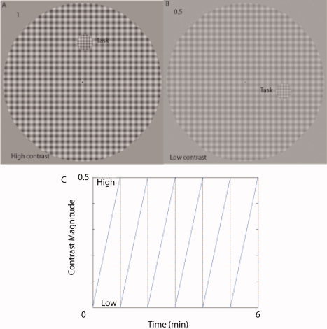
A: Stimuli (1c/d; 2 Hz) used in this study, at highest contrast (50%). B: Stimuli used in this study, a low contrast (20% shown here for illustrative purposes only). C: Phased encoded design, contrast of the stimuli change linearly with time, from 0.5 to 0, and repeated for six cycles, each cycle taking 1 min to complete. [Color figure can be viewed in the online issue, which is available at www.interscience.wiley.com.]
Image Acquisition
A Siemens 1.5T Magnetom scanner used to collect both anatomical and functional images of subjects DV, GN, HP, ML, and normal MG, while the anatomical and functional images of the other subjects were collected using a GE 1.5T Signa scanner.
For the Siemens scanner, a rectangular coil (14.5″ × 6.5″), head coil (circularly polarized transmit and receive), and a T1‐weighted sequence (TR = 22 ms; TE = 10 ms; flip angle = 30°) were used to acquire 176 sagittal slices of 256 × 256 mm2 of anatomical image. Functional scans for each subject were collected using a surface coil (circularly polarized, receive only) positioned beneath the subject's occiput. Each functional imaging session was preceded by a surface coil anatomical scan (identical to the head coil anatomical sequence, except that 80 × 256 × 256 sagittal images of slice thickness 2 mm were acquired) to later co‐register the data with the more homogeneous head‐coil image. Functional scans were multislice T2*‐weighted, gradient‐echo, planar images (GE‐EPI, TR = 3.0 s, TE = 51 ms, flip angle = 90°). Image volumes consisted of 30 slices orthogonal to the calcarine sulcus for retinotopic mapping, whereas images were collected parallel to the carlarine sulcus for the contrast experiment. The field of view was 256 × 256 mm2 and the matrix size was 64 × 64 with a thickness of 4 mm giving a voxel size of 4 × 4 × 4 mm.
For the GE scanner, a Quad head coil and a T1‐weighted sequence (TR = 82 ms; TE = 32 s; flip angle = 15°) were used to acquire 124 sagittal slices of 256 × 256 mm2 of anatomical image. Functional scans for each subject were collected using the same head coil. As described earlier, each functional imaging session was preceded by an anatomical scan (TR = 50 ms; TE = 10 ms; flip angle = 65°) where 59 × 512 × 512 sagittal images of slice thickness 2 mm were acquired. Functional scans were also multislice T2*‐weighted, gradient‐echo, planar images (TR = 3.0 s, TE = 50 ms, flip angle = 90°). The field of view was 240 mm × 240 mm2, and all other parameters were the same as those used for the Siemens scanner.
For the retinotopic mapping, there were four acquisition runs for each eye (two eccentricity, two polar angle) each consisting of 128 image volumes acquired at 3‐s intervals for both the fixing and AE of amblyopes. For the contrast experiment, there were four acquisition runs for each eye, each consisting of 128 volumes acquired at 3‐s intervals for both the fixing and AE of amblyopes. Runs were alternated between the eyes in each case while the subject performed a task [Li et al., 2007b]. The task for the retinotopic mapping scans was to detect a coherent patch of checks (either regular in luminance, or chromatic content) that appeared randomly in a random position in the stimulus. The task for the contrast experiment was to maintain central fixation and detect a region of higher spatial frequency texture presented somewhere in the stimulus field. Responses were collected using a button box.
Data Analysis
Anatomical images
The global T1‐weighted aMRI scans were corrected for intensity nonuniformity [Sled et al., 1998] and automatically registered [Collins et al., 1994] in a stereotaxic space [Talairach and Tournoux, 1988] using a sterotaxic model of 305 brains [Evans et al., 1993]. The surface‐coil aMRI, acquired in the same session as the functional images, was aligned with the head‐coil aMRI, thereby allowing an alignment of the functional data with a head‐coil MRI and subsequently stereotaxic space. A validation of this method was described in a previous study [Dumoulin et al., 2003]. Boundaries of V1–V4 were defined by the visual field sign from the aMRI and retinotopic mapping functional data. All processing steps were automatic, and all data are presented in standard stereotaxic space. Analysis was performed separately for each voxel within each ROI for left and right hemisphere. % BOLD values for each voxel were then averaged for each visual area and across hemispheres to derive a single average % BOLD change for each area.
Functional Images
Dynamic motion correction for functional image time series for each run and for different runs were simultaneously realigned by fmri_preprocess function provided by MINC tools (http://www.bic.mni.mcgill.ca/). The first eight scans of each functional run were discarded due to start‐up magnetization transients in the data. Then the time series of BOLD signal change was normalized temporally, i.e.:
| (1) |
where
 is the normalized BOLD‐fMRI time series, S(i) is the raw fMRI time series, i is the sampled time point (image frame), S is the mean value of the series, and σ is the standard deviation of the time series. Because of the nature of phase‐encoded experimental design, fast Fourier transformation was used to get the fundamental frequency of the normalized BOLD response
 . To detect the brain activation caused by modulations in contrast effect (Fig. 1C), for each voxel, a design matrix was constructed by combining the fundamental‐frequency response and low‐frequency drift effects and t‐statistics were used to quantify the effect size (see Fig. 2 and Appendix of Li et al. [2007a]). Different runs for each eye were combined using the mixed model [Seber and Lee, 2003; Worsley et al., 2002].
Figure 2.
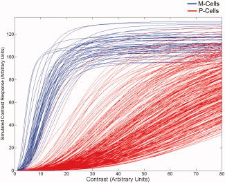
An example of one of the simulated M‐ and P‐cell CRF populations used in the model (without simulated cell loss). On the ordinate is the contrast response (arbitrary units). On the abscissa is the contrast of the stimulus (also in arbitrary units).
We averaged three time points corresponding to the three highest contrasts (45%, 47.5%, 50%) presented as a measure of the high‐contrast response in Eq. (1), and the time points corresponding to the three lowest contrasts (2.5%, 5%, 7.7%) as the low‐contrast response [Fig. 1 and Eq. (1)]. BOLD percentage change was derived at selected time points, so that responses to high‐ and low‐contrast stimulation could be compared. The paired t test was used to test the difference of % BOLD signal change and brain activation quantified by the T statistics [T(117) > 1.98, P < 0.05, two‐tailed t test) between the eyes.
Psychophysics
Eye occlusion and Dominance
To test monocular function, we occluded either the fixing or fellow AE with a black patch designed to exclude all light. This was done for both the psychophysical testing and for the brain imaging. Under these conditions, there is no binocularly mediated suppression of the AE, because all pattern vision in the good eye has been abolished [Harrad and Hess, 1992], and thus our estimates of the reduced activation in the brains of amblyopes are a conservative one as it does not include a binocularly suppressive component. Eye dominance was assessed using a standard sighting test [Rosenbach, 1903].
Neural Modeling
The population‐based model we used to simulate relative contrast loss as a function of under‐represented M‐ or P‐cells consisted of generating sets of contrast response functions (CRFs) for sub‐sets of cells and selectively eliminating different proportions of either cell type to predict the contrast loss attributed to loss of either cell type for an AE. The simulated responses for both M‐ and P‐cells were based on a modified version of the well known Naka–Rushton equation. Specifically, Naka and Rushton [1966] have shown that the Michaelis–Menton function possessing an exponent, n, of unity can be used to describe the intensity response function of individual neurons in fish retinae, with the response increasing with the intensity of the stimulus in a nonlinear (in this case hyperbolic) fashion, expressed as:
| (2) |
where R is the response amplitude elicited by the intensity, I, of the stimulus, R MAX is the maximum response of the mechanism, and σ is the semisaturation constant (i.e., illumination at which R reaches R MAX/2). Note that this equation is approximately linear when I < σ, and as I extends beyond this value, increments of I evoke minimal changes in R, that is, Eq. (1) describes a mechanism that saturates. The hyperbolic function described earlier has also been shown to describe the CRF of many neurons in striate cortex of cats and primates [e.g., Albrecht and Hamilton, 1982] by replacing intensity, I, with contrast, C. Equation (2) can be modified to possess a contrast gain component by requiring the response, R, change not only as a function of C, but also as a function of σ multiplied by a gain factor, g [e.g., Shapley and Enroth‐Cugell, 1984], stated formally as
| (3) |
Population of M‐ and P‐cell CRFs were generated by using the means of the parameters reported by Albrecht and Hamilton [1982] for the hyperbolic fits to their data as a bench mark and randomly (normal distribution) varying those values with respect to peak response (R max), semisaturation constant (σ), and exponent (n) about the reported means. Because the gain factor, g, should also be expected to vary about a mean, we randomly (normal distribution) varied g around a mean of 0.3 for the M‐cell population and 3.0 for the P‐cell population. Figure 2 plots the CRFs for a population of 500 cells following the 8:1 ratio [Shapley and Perry, 1986] with parameters as outlined earlier. The CRFs for the M‐ and P‐cells shown in Appendix Figure 1 follow very closely those reported in the literature for these cell types [c.f. Purpura, Kaplan, Shapley, 1988; Benardete et al., 1997, 1999].
The model described here is based only on simulated responses from within the effective response range of the CRFs. To illustrate which cells in the simulated population shown in Appendix Figure 1 exhibit effective responses for a given level contrast, we count the number of cells exhibiting an effective response to contrasts between 0 and 80, which yields the response histogram shown in Figure 3.
Figure 3.
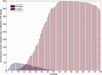
Number of simulated neurons exhibiting an effective contrast response for a range of arbitrary contrast values. On the ordinate is the number of neurons encountered in each simulated cell subpopulation yielding an effective contrast response. On the abscissa is the contrast of the stimulus (arbitrary units).
Using the CRF population simulation method described earlier, we simulated contrast loss by selectively “silencing” small percentages of the CRFs for the entire population, which simply involved removing a subset of CRFs from the population. Simulated contrast loss is defined by the summed activity of M or P cells in a fellow‐fixing eye (FFE, where no selective loss was simulated) relative to an AE (where selective cell loss was induced) across the range of contrasts where both cell types are active (Fig. 3). The difference in the total summed activity between each subpopulation cell type between each eye was assessed with standard independent samples t‐tests. For example, for simulating P‐cell loss in an AE, a population of CRFs was generated for each eye and a given percentage of P‐cells was removed from the AE population. The summed total of effective range responses for the AE and FFE was assessed for 10 different simulations, and the average difference in simulated output was assessed via the t‐statistic mentioned earlier. The same procedure was carried out for the M‐cell subpopulation where no selective cell loss was induced. This process was carried out for each “simulated participant” (n = 14) and then repeated 10 more times to get standard error. Thus, each simulated participant had an averaged joint t‐statistic for P‐cells and M‐cells (plotted in Fig. 4). For simulating M‐cell loss, the same procedure was used, only selective silencing was applied to the M‐cell CRF population for the AE. It is important to note that the percentage of simulated loss for both M‐ and P‐cells for the AE reported in the text should not be taken as a literal estimate as they are based on the model CRF population parameters described earlier.
Figure 4.
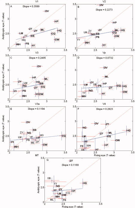
Magnitude responses to the full cycle of stimulation for the contrast‐varying stimulus are given for different visual areas for a group of amblyopes. The Y‐axis is the response for the amblyopic eye (T‐values) and the X axis is the response of the fellow fixing eye (T‐values). The dashed line has a slope of unity and the solid line is the best fit () to the amblyopic data as a whole. Data for individual subjects are given by initials (see Table I), and initials enclosed by a dashed box indicate responses for an individual that are significantly reduced (T > 1.965: P < 0.05, two‐tailed t‐test) for the amblyopic eye. The following data overlap occurs; V1 (YY&NG), V2 (LM&YY), Vp (SB&PB), V3a (YY&ZF), and V4 (WH&SB). Responses for different retinotopic areas are given (A–G).
RESULTS
Figure 4 shows a comparison of the magnitude responses averaged across one cycle of the stimulus (i.e., across all stimulus contrasts), quantified in terms of T‐value, for the amblyopic and fellow fixing eye of all our amblyopic subjects for the phase‐encoded contrast stimulus for the retinotopic visual areas. The dashed line has unity slope and data falling on or near this line indicates comparable responses for fixing and AEs across the range of contrast through which our stimulus varied (i.e., 0–50%). The solid line is the best fit to the amblyopic population as a whole, and the data for each subject are shown by initials. Initials enclosed by a dashed box indicates responses that are significantly reduced (t‐test; P < 0.05) from that of the fellow fixing eye. There is variability across the population with not all amblyopes exhibit reduced magnitude responses for the phase‐encoded stimulus, consistent with previous studies [Barnes et al., 2001; Conner et al., 2007a; Li et al., 2007a]. For the population as a whole, the amblyopic response is significantly reduced only in area V1 (T = 2.1993, df = 28; P < 0.05) and Vp (T = 2.1141, df = 28; P < 0.05); however, individual subjects display significant reductions (T > 1.965: P < 0.05, two‐tailed t‐test) in response for the phase‐encoded stimulus in all visual areas (e.g., in area V1, ML, HP, SB, YF, HQ, CQ, CW; area V2, WH, CQ, ML, HQ, CW, YF; area V3, ML, SB, ZF, CQ, YF, CW; area Vp, ZF, CQ, HQ, CW, YF; area V3a, WH, CW, CQ, HP, ZF, ML; area V4, HP, HQ; area MT, HQ, HP, CQ. Because a reduction in response to this contrast varying stimulus could in principle be due to reduced responses at low contrast or reduced responses at high contrast or a combination of the two, we derived % BOLD responses from selected time points on our stimulus cycle to assess the contrast dependence of the fMRI deficit.
Figure 5 shows a comparison of the fMRI responses between the eyes of normal subjects in terms of the difference in the % BOLD change. The Y axis is the interocular difference in the BOLD signal change for the high‐contrast response (dominant eye–nondominant eye). The X axis is the same measurement for the low‐contrast response (dominant eye–nondominant eye). The responses for both dominant and nondominant eye stimulation for the high‐contrast stimuli were statistically greater (see Statistical Analysis section below) than those for the low‐contrast stimuli in all visual areas, as one would expect from the contrast dependence of the BOLD response [Goodyear and Menon, 1998]. However, because the dominant and nondominant eye responses were of a comparable magnitude for both the low‐ and high‐contrast stimuli, the interocular differences in response magnitude cluster around the origin, although there is some variability, showing that there is similar activation when the cortex is driven by either eye, irrespective of stimulus contrast.
Figure 5.
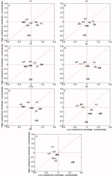
% BOLD change for the normal control subjects. Y axis is the difference in the BOLD signal change for high contrasts (dominant eye–nondominant eye). X axis is the difference for low contrasts (dominant eye–nondominant eye). Results are shown for the different retinotopic visual areas. Responses cluster around the origin, although there is some variability. Responses for different retinotopic areas are given (A–G).
Similar results for a group of amblyopes (strabismic and anisometropic) are seen in Figure 6. We confirmed that significant responses were obtained from both the low‐ and the high‐contrast stimuli in isolation for both fixing and fellow AE stimulation. Also, for the fixing eye, the responses for the high‐contrast stimuli were larger than those for the low‐contrast stimuli (see Statistical Analysis section below) for all visual areas, though this was not the case for the AE. Here, the interocular differences in response are larger than found for normal observers owing to the fact that the response due to the AE stimulation is reduced. Furthermore, these interocular differences in response are greater for high‐contrast stimuli. This is true for the majority of the retinotopic visual areas.
Figure 6.
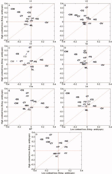
% BOLD change for the amblyopic subjects. Y axis is the difference in the BOLD signal change for high contrasts (fixing eye–amblyopic eye). X axis is a comparable comparison at the low contrasts (fixing eye–amblyopic eye). Responses for the amblyopes extend further out from the origin (compared with Fig. 2, particularly into the upper left corner reflecting a greater loss for high‐contrast stimuli. The following data overlap occurs; V1(WH&ML), (PB&HP&YY), V2 (CW&ZY), (YY&WH), Vp (HP&WH&YP&YY), V3a(YY&HQ), V4(ZY&PB), (WH&YF), MT(ZY&PB), and (WH&YF). Responses for different retinotopic areas are given (A–G).
Figure 7 shows the averaged activation maps for our amblyopic population on a standardized flattened cortical surface with the standardized boundaries [Van Essen, 2005] of the early visual areas drawn in for reference. In Figure 7A, the difference in the activation between fixing and AEs is shown for only high‐contrast stimuli. In Figure 7B, the comparable deficit is displayed for low‐contrast stimuli. In Figure 7C, the regional overlap between the high‐ and low‐contrast deficits is displayed. The deficit for high‐contrast stimuli is extensive and affects all early cortical areas. The low‐contrast deficit is limited to peripheral parts of the visual field in V1 and is of much lesser magnitude.
Figure 7.
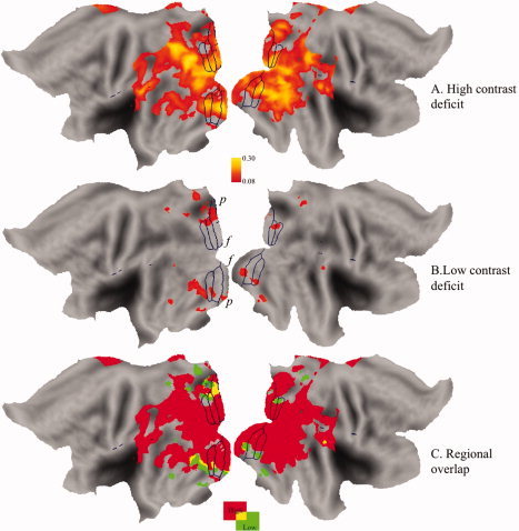
The averaged functional activation data for the high contrast (A) and low contrast (B) conditions on an averaged, standardized flattened cortex (Van Essen DC (2001): J Am Med Infor Soc 8:443–459) with standardized areal boundaries for reference. f denotes the fovea and p the periphery.
Statistical Analysis
A repeated measures ANOVA (degrees of freedom corrected for sphericity using the Huynh–Feldt correction) conducted on the amblyopic participant data revealed a significant interaction between contrast (high vs. low) and eye (amblyopic vs. nonamblyopic), F(1,14) = 6.14, P = 0.027, showing that across all visual areas, there was a reliable difference between the two eyes in terms of the BOLD response to the low‐ and high‐contrast stimuli. Figure 8 clearly demonstrates that the difference is driven by a loss of the high‐contrast response in the AE.
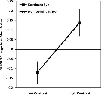
Figure 8.
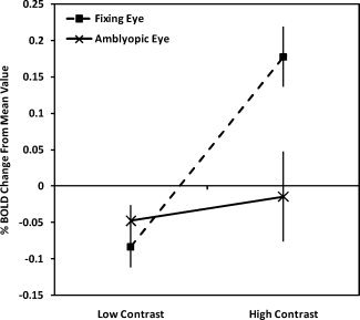
Amblyopic participants' averaged BOLD response change relative to the mean collapsed across visual areas for the low‐ and high‐contrast conditions
As expected, the same analysis conducted on the control participants showed no such interaction with both the dominant and the nondominant eye (Fig. 9) responding comparably. The main effect of contrast (low vs. high) was close to significance for the control group F(1,6) = 5.19, P = 0.06 and significant for the amblyopic group F(1,14) = 21.23, P = 0.0004. To assess whether these effects differed by visual area, additional ANOVA analyses were conducted for each visual area separately. For the amblyopic group, significant interactions between contrast and eye were found for every visual area as was a significant main effect of contrast (P < 0.05 for all). For the control group, interactions between contrast and eye were not present for any visual area as expected from Figure 9. Only V1 showed a significant main effect of contrast, F(1,6) = 6.73, P = 0.041; however, all other areas showed marginal main effects of contrast with P values ranging from 0.055 to 0.094. No significant differences were found between the responses of fixing and AEs of strabismics compared with anisometropes.
Figure 9.
Control participants' averaged BOLD responses change relative to the mean collapsed across visual areas for the low‐ and high‐contrast conditions
Model Simulations
To relate this greater loss of cortical function for high contrasts in strabismic amblyopes to the function of M‐ and P‐pathways, we developed predictions from a population‐based model simulation, based on the available physiology of M‐ and P‐cell losses. Using a modified version of the Naka–Rushton equation (described in the Methods section), we simulated populations of M‐ and P‐cell CRFs, with each neuron's CRF described with parameters that were randomly (normal distribution) distributed around the optimal values reported by Albrecht and Hamilton [1982]. The model presupposes that the relative numbers of P‐ and M‐cells are in the ratio of 8:1 [Shapley and Perry, 1986] and assumes that the fellow fixing eye has a normal compliment of P‐ and M‐cells. However, for the AE, we simulated cell loss by selectively “silencing” different proportions of either M‐ or P‐cells. By comparing the total summed activity for each cell subpopulation between each eye in response to stimulus contrast, we generated predictions of contrast loss (refer Fig. 10) as a function of P‐ or M‐cell loss for % BOLD response (see Methods section for more details). Plotted in Figure 5 are joint t‐statistics associated with the difference in the total summed simulated CRF response between fellow fixing and AEs at low‐contrast responses and high contrasts. Predictions are given for 2° of simulated P‐cell loss and for 2° of simulated M‐cell loss. The simulations show that a selective loss at low contrasts would be expected from a loss of M‐cells, owing to their higher contrast gain and that a selective loss at high contrasts would be expected from a loss of P‐cells, owing to their low contrast gain.
Figure 10.
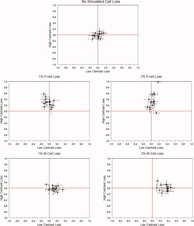
Model simulations of the contrast loss from M‐ and P‐cell dysfunction. The model description is given in the Appendix, and it involves differential numbers of M and P‐cells as well as differences in their contrast gains. A selective P‐cell loss would affect higher contrasts whereas a selective M‐cell loss would affect low contrasts. The percentage of simulated loss for both M‐ and P‐cells for the AE reported in the text should not be taken as a literal estimate as they are based on the model CRF population parameters described in the Appendix. Nonetheless, the simulated contrast loss shown here for the P‐cell loss predicts the contrast loss shown in the fMRI data.
DISCUSSION
The main finding is that the fMRI deficit is more pronounced at high compared with low contrasts in strabismic, and nonstrabismic anisometropic, amblyopes. This involves a number of the early visual areas, not just V1. At first, it seems counter‐intuitive that the contrast loss in strabismic amblyopia could selectively affect high contrasts as there is a well‐documented threshold anomaly [Gstalder and Green, 1971; Hess and Howell, 1977; Levi and Harwerth, 1977] and normal contrast matching for suprathreshold contrast [Hess and Bradley, 1980]. However, the behavioral threshold losses are restricted to high‐spatial frequencies (not tested here) and furthermore, there is no compelling support for the proposition that fMRI losses are greater at high‐spatial frequencies [Barnes et al., 2001; Muckli et al., 2006; Hess et al., 2009]. This may be because behavioral thresholds are supported by the most sensitive cells, and, if these are few in number, their response may not be well represented in the mass fMRI response. To this extent, the sensitivity of fMRI may not be the same for cellular loss confined to stimuli of just low and just high contrasts. Here, we concentrate on the processing of intermediate spatial frequencies where human contrast sensitivity is best, but where there is behavioral evidence both in humans [Baker et al., 2008; Harrad and Hess, 1992; Hess et al., 1983] and monkeys [Kiper and Kiopes, 1994] for amblyopic processing deficits. We show that the fMRI deficits in this spatial frequency range are greater at high contrasts.
Selective P‐Cell Loss Hypothesis
Assuming that our model predictions based on the total summed difference in response are reflected in fMRI activity, how realistic are the model predictions? Merigan and colleagues have lesioned both P‐ and M‐cell populations in the geniculate and documented contrast sensitivity losses [Merigan et al., 1991; Merigan and Maunsell, 1990, 1993]. It is clear from their results that the threshold effects are dependent on the spatio‐temporal properties of the stimuli used. In our case, the use of a spatial frequency of 1c/d and temporal frequency of 2 Hz would have been expected to produce a larger contrast threshold loss for an M‐cell lesion than for a P‐cell lesion [Merigan and Maunsell, 1993], which is in line with our model predictions. It is not possible to validate our prediction that a higher contrast loss would be expected from a P‐cell lesion, because there are no current behavioral measures of suprathreshold contrast function from such selective lesions. Our conclusions are consistent with those of a recent study of the fMRI responses of the LGN in strabismic amblyopes showed a greater deficit for red/green stimuli, consistent with a selective P‐cell deficit [Hess et al., 2008]. They are also consistent with a recent single case study [Miki et al., 2008] in which different spatio‐temporal stimuli were used to examine whether the fMRI loss was selective for M‐ and/or P‐cell function in an anisometropic amblyope. They concluded, like that of this study, that the loss of function may be greater for P‐cell activity.
Striate Versus Extra‐Striate Deficits
The model outlined earlier is based on responses at the level of the lateral geniculate nucleus where the different contrast gain properties of M‐ and P‐cells have been delineated using single‐cell neurophysiology [Kaplan and Shapley, 1986]. Because the fMRI signal reflects local field potentials more than it does action potentials [Logothetis et al., 2001], it tells us more about the synaptic input to an area rather than its spiking output. This being the case, the model is particularly relevant to V1 as it receives all its input from the LGN and where at the input level the M‐ and P‐inputs from the geniculate are segregated by layer (i.e. 4cB and 4Ca) and have been shown to exhibit reduced responses when driven by the AE [Hess et al., 2009a].
It is interesting that we find similar high‐contrast deficits in extra‐striate cortex, because it is known that CRFs in extra‐striate cortex exhibit greater high‐contrast saturation than those of V1 [Hall et al., 2005; Tootell et al., 1998]. One possibility is that our findings reflect a loss of P cell processing at an early level in the pathway where M and P cell inputs are separate (i.e., lgn or layer 4C of V1). Under these conditions, a P‐cell loss would be expected to propagate throughout the visual pathway and influence cellular responses to higher contrasts.
Relative P‐and M‐Cell Loss in Amblyopia
There is no unified view from the psychophysical literature on whether P‐ or M‐cell function is selectively affected in amblyopia. Some studies argue for a selective P‐cell deficit [Altmann and Singer, 1986], others for a selective M‐cell deficit [Previc, 1989] and others for combined M‐ and P‐deficits [Buckingham et al., 1991]. A similar divergence of opinion is seen in the neurophysiological literature with selective P‐ [Ikeda and Wright, 1974; Kubova et al., 1996] and M‐cell losses [Sherman et al., 1975; Yin et al., 1997] claimed. In amblyopia, there are deficits for the detection of static‐contrast stimuli as well as for the global processing of both motion [Aaen‐Stockdale and Hess, 2008; Simmers et al., 2003, 2006], spatial position [Gingras et al., 2005a, b; Hess and Holliday, 1992], and form [Mansouri and Hess, 2006; Simmers et al., 2005]. It is therefore likely that both P‐cell and M‐cell‐mediated functions are affected at different levels in the pathway. However, the lower‐level contrast processing deficit may reflect a differential P‐cell loss for two reasons. First, the behavioral contrast sensitivity deficits are only present for static‐ or low‐temporal frequency stimulation [Hess et al., 1978]. Second, a recent study [Hess et al., 2008] has shown reduced fMRI responses from the lateral geniculate nucleus in amblyopic individuals for red/green stimuli, suggestive of a selective loss of P‐cell function early in the pathway.
REFERENCES
- Aaen‐Stockdale C, Hess RF ( 2008): The amblyopic deficit for global motion is spatial scale invariant. Vision Res 48: 1965–1971. [DOI] [PubMed] [Google Scholar]
- Albrecht DG, Hamilton DB ( 1982): Striate cortex of monkey and cat: Contrast response function. J Neurophysiol 48: 217–237. [DOI] [PubMed] [Google Scholar]
- Algaze A, Roberts C, Leguire L, Schmalbrock P, Rogers G ( 2002): Functional magnetic resonance imaging as a tool for investigating amblyopia in the human cortex: A pilot study. J AAPOPS 6: 300–308. [DOI] [PubMed] [Google Scholar]
- Altmann L, Singer W ( 1986): Temporal integration in amblyopic vision. Vision Res 26: 1959–1968. [DOI] [PubMed] [Google Scholar]
- Anderson SA, Holliday IE, Harding GF ( 1999): Assessment of cortical dysfunction in human strabismic amblyopia using magnetoencephalography. Vision Res 39: 1723–1738. [DOI] [PubMed] [Google Scholar]
- Baker DH, Meese TS, Hess RF ( 2008): Contrast masking in strabismic amblyopia: Attenuation, noise, interocular suppression and binocular summation. Vision Res 48: 1625–1640. [DOI] [PubMed] [Google Scholar]
- Barnes GR, Hess RF, Dumoulin SO, Achtman RL, Pike GB ( 2001): The cortical deficit in humans with strabismic amblyopia. J Physiol (Lond) 533: 281–297. [DOI] [PMC free article] [PubMed] [Google Scholar]
- Buckingham T, Watkins R, Bansal P, Bamford K ( 1991): Hyperacuity thresholds for oscillatory movement are abnormal in strabismic and anisometropic amblyopes. Optom Vis Sci 68: 351–356. [DOI] [PubMed] [Google Scholar]
- Choi MY, Lee KM, Hwang JM, Choi DG, Lee DS, Park KH, Yu YS ( 2001): Comparison between anisometropic and strabismic amblyopia using functional magnetic resonance imaging. Br J Ophthalmol 85: 1052–1056. [DOI] [PMC free article] [PubMed] [Google Scholar]
- Collins DL, Neelin P, Peters TM, Evans AC ( 1994): Automatic 3D intersubject registration of MR volumetric data in standardized Talairach space. J Comput Assist Tomopgr 18: 192–205. [PubMed] [Google Scholar]
- Conner IP, Mendola JD ( 2005): What does an amblyopic eye tell human visual cortex? Sarasota, Fl. J Vision. 5( 8): 295a. [Google Scholar]
- Conner IP, Odom JV, Schwartz TL, Mendola JD ( 2007a): Monocular activation of V1 and V2 in amblyopic adults measured with functional magnetic resonance imaging. J AAPOS 11: 341–350. [DOI] [PMC free article] [PubMed] [Google Scholar]
- Conner IP, Odom JV, Schwartz TL, Mendola JD ( 2007b): Retinotopic maps and foveal suppression in the visual cortex of amblyopic adults. J Physiol 583 ( Pt 1): 159–173. [DOI] [PMC free article] [PubMed] [Google Scholar]
- Demer JL ( 1997): Positron‐emisson tomographic study of human amblyopia with use of defined visual stimuli. J AAPOPS 1: 158–171. [DOI] [PubMed] [Google Scholar]
- Demer JL, von Noorden GK, Volkow ND, Gould KL ( 1988): Imaging of cerebral flow and metabolism in amblyopia by positron emission tomography. Am J Ophthalmol 105: 337–347. [DOI] [PubMed] [Google Scholar]
- Dumoulin SO, Hoge RD, Achtman RL, Baker CL, Hess RF, Evans AC ( 2000): Volumetric retinotopic mapping without cortical surface reconstruction. NeuroImage 11: s613. [Google Scholar]
- Dumoulin SO, Hoge RD, Baker CL, Hess RF, Achtman RL, Evans AC ( 2003): Automatic volumetric segmentation of human visual retinotopic cortex. NeuroImage 18: 576–587. [DOI] [PubMed] [Google Scholar]
- Evans AC, Collins DL, Mills SR, Brown ED, Kelly RL, Peters TM ( 1993): 3D statistical neuroanatomical models from 305 MRI volumes; p 1813–1817. [Google Scholar]
- Gingras G, Mitchell DE, Hess RF ( 2005a): Haphazard neural connections underlie the visual deficits of cats with strabismic or deprivation amblyopia. Eur J Neurosci 22: 119–124. [DOI] [PubMed] [Google Scholar]
- Gingras G, Mitchell DE, Hess RF ( 2005b): The spatial localization deficit in visually deprived kittens. Vision Res 45: 975–989. [DOI] [PubMed] [Google Scholar]
- Goodyear BG, Menon RS ( 1998): Effect of luminance contrast on BOLD fMRI response in human primary visual areas. J Neurophysiol 79: 2204–2207. [DOI] [PubMed] [Google Scholar]
- Goodyear BG, Nicolle DA, Humphrey GK, Menon RS ( 2000): BOLD fMRI response of early visual areas to perceived contrast in human amblyopia. J Neurophysiol 84: 1907–1913. [DOI] [PubMed] [Google Scholar]
- Gstalder RJ, Green DG ( 1971): Laser interferometric acuity in amblyopia. J Pediatr Ophthalmol 8: 251–256. [Google Scholar]
- Hall SD, Holliday IE, Hillebrand A, Furlong PL, Singh KD, Barnes GR ( 2005): Distinct contrast response functions in striate and extra‐striate regions of visual cortex revealed with magnetoencephalography (MEG). Clin Neurophysiol 116: 1716–1722. [DOI] [PubMed] [Google Scholar]
- Harrad RA, Hess RF ( 1992): Binocular integration of contrast information in amblyopia. Vision Res 32: 135–2150. [DOI] [PubMed] [Google Scholar]
- Hess RF, Bradley A ( 1980): Contrast coding in amblyopia is only minimally impaired above threshold. Nature 287: 463–464. [DOI] [PubMed] [Google Scholar]
- Hess RF, Holliday IE ( 1992): The spatial localization deficit in amblyopia. Vision Res 32: 1319–1339. [DOI] [PubMed] [Google Scholar]
- Hess RF, Pointer JS ( 1985): Differences in the neural basis if human amblyopias: The distribution of the anomaly across the visual field. Vision Res 25: 1577–1594. [DOI] [PubMed] [Google Scholar]
- Hess RF, Howell ER, Kitchin JE ( 1978): On the relationship between pattern and movement perception in strabismic amblyopia. Vision Res 18: 375–377. [DOI] [PubMed] [Google Scholar]
- Hess RF, Bradley A, Piotrowski L ( 1983): Contrast‐coding in amblyopia. I. Differences in the neural basis of human amblyopia. Proc R Soc Lond B Biol Sci 217: 309–330. [DOI] [PubMed] [Google Scholar]
- Hess RF, Thompson B, Gole G, Mullen KT ( 2008): The LGN deficit in amblyopia is selective for parvocellular function. Washington: Society for Neuroscience. [Google Scholar]
- Hess RF, Thompson B, Gole G, Mullen KT ( 2009a): Deficient responses from the lateral geniculate nucleus in humans with amblyopia. Eur J Neurosci 29: 1064–1070. [DOI] [PMC free article] [PubMed] [Google Scholar]
- Hess RF, Li X, Mansouri B, Thompson B, Hansen B ( 2009b): Selectivity as well as sensitivity characterizes the cortical spatial frequency deficit in amblyopia. Human brain mapping (in press). [DOI] [PMC free article] [PubMed] [Google Scholar]
- Ikeda H, Wright MJ ( 1974): Is amblyopia due to inappropriate stimulation of the ‘sustained’ pathway during development. Br J Ophthal 58: 165–175. [DOI] [PMC free article] [PubMed] [Google Scholar]
- Imamura K, Richter H, Lennerstrand G, Rydberg A, Andersson J, Schneider H, Watanabe Y, Langstrom B ( 1997): Reduced activity in the extra‐striate visual cortex of individuals with strabismic amblyopia. Neurosci Lett 225: 173–176. [DOI] [PubMed] [Google Scholar]
- Kabasakal L, Devranoglu K, Arslan O, Erdil TY, Sonmezoglu K, Uslu I, Tolunm H, Isitman AT, Ozker K, Onsel C ( 1995): Brain SPECT evaluation of the visual cortex in amblyopia. J Nucl Med 36: 1170–1174. [PubMed] [Google Scholar]
- Kaplan E, Shapley RM ( 1986): The primate retina contains two types of ganglion cells, with high and low contrast sensitivity. Proc Natl Acad Sci USA 83: 2755–2757. [DOI] [PMC free article] [PubMed] [Google Scholar]
- Kiper DC, Kiopes L ( 1994): Suprathreshold contrast sensitivity in experimentally strabismic monkeys. Vision Res 34: 1575–1583. [DOI] [PubMed] [Google Scholar]
- Kubova Z, Kuba M, Juran J, Blakemore C ( 1996): Is the motion system relatively spared in amblyopia? Evidence from cortical evoked potentials. Vision Res 36: 181–190. [DOI] [PubMed] [Google Scholar]
- Lee KM, Lee SH, Kim NY, Kim CY, Sohn JW, Choi MY, Choi DG, Hwang JM, Park KH, Lee DS, Yu YS, Chang KH ( 2001): Binocularity and spatial frequency dependence of calcarine activation in two types of amblyopia. Neurosci Res 40: 147–153. [DOI] [PubMed] [Google Scholar]
- Levi M, Harwerth RS ( 1977): Spatio‐temporal interactions in anisometropic and strabismic amblyopia. Invest Ophthalmol Vis Sci 16: 90–95. [PubMed] [Google Scholar]
- Li X, Dumoulin SO, Mansouri B, Hess RF ( 2007a): Cortical deficits in human amblyopia: Their regional distribution and their relationship to the contrast detection deficit. Invest Ophthal Vis Sci 48: 1575–1591. [DOI] [PubMed] [Google Scholar]
- Li X, Dumoulin SO, Mansouri B, Hess RF ( 2007b): The fidelity of the cortical retinotopic map in human amblyopia. Eur J Neurosci 25: 1265–1277. [DOI] [PubMed] [Google Scholar]
- Logothetis NK, Pauls J, Augath M, Trinath T, Oeltermann A ( 2001): Neurophysiological investigation of the basis of the fMRI signal. Nature 412: 150–157. [DOI] [PubMed] [Google Scholar]
- Mansouri B, Hess RF ( 2006): The global processing deficit in amblyopia involves noise segregation. Vision Res 46: 4104–4117. [DOI] [PubMed] [Google Scholar]
- Merigan WH, Maunsell JH ( 1990): Macaque vision after magnocellular lateral geniculate lesions. Vis Neurosci 5: 347–352. [DOI] [PubMed] [Google Scholar]
- Merigan WH, Maunsell JH ( 1993): How parallel are the primate visual pathways? Annu Rev Neurosci 16: 369–402. [DOI] [PubMed] [Google Scholar]
- Merigan WH, Katz LM, Maunsell JH ( 1991): The effects of parvocellular lateral geniculate lesions on the acuity and contrast sensitivity of macaque monkeys. J Neurosci 11: 994–1001. [DOI] [PMC free article] [PubMed] [Google Scholar]
- Miki A, Siegfried J, Liu C‐S, Modestino EJ, Liu G ( 2008): Magno‐and parvocellular visual cortex activation in anisometropia, as studied with functional magnetic resonance imaging. Neuro‐Ophthalmol 32: 187–193. [Google Scholar]
- Muckli L, Kiess S, Tonhausen N, Singer W, Goegel R, Sireteanu R ( 2006): Cerebral correlates of impaired grating perception in individual psychophysically assessed human amblyopes. Vision Res 46: 506–526. [DOI] [PubMed] [Google Scholar]
- Previc FH ( 1989): Functional specialization in the lower and upper visual fields; its ecological origins and neurophysiological implications. Behav Brain Sci 13: 519–575. [Google Scholar]
- Rosenbach O ( 1903): Ueber monokulare Vorherrschaft beim binikularen Sehen. Munchener Medizinische Wochenschriff 30: 1290–1292. [Google Scholar]
- Seber GAF, Lee AJ ( 2003): Linear regression analysis, 2nd ed. Wiley‐Interscience, New York: pp 97–118. [Google Scholar]
- Shapley R, Perry VH ( 1986): Cat and monkey retinal ganglion cells and their visual functional roles. Trends Neurosci 9: 229–235. [Google Scholar]
- Sherman SM, Wilson JR, Guillery RW ( 1975): Evidence that binocular competition affects the postnatal development of Y‐cells in the cat's lateral geniculate nucleus. Brain Res 100: 441–444. [DOI] [PubMed] [Google Scholar]
- Simmers AJ, Ledgeway T, Hess RF, McGraw PV ( 2003): Deficits to global motion processing in human amblyopia. Vision Res 43: 729–738. [DOI] [PubMed] [Google Scholar]
- Simmers AJ, Ledgeway T, Hess RF ( 2005): The influences of visibility and anomalous integration processes onb the perception of global spatial form versus motion in human amblyopia. Vision Res 45: 449–460. [DOI] [PubMed] [Google Scholar]
- Simmers AJ, Ledgeway T, Mansouri B, Hutchinson CV, Hess RF ( 2006): The extent of the dorsal extra‐striate deficit in amblyopia. Vision Res 46: 2571–2580. [DOI] [PubMed] [Google Scholar]
- Sled JG, Zijdenbos AP, Evans AC ( 1998): A non‐parametric method for automatic correction of intensity non‐uniformity in MRI data. IEEE Trans Med Imag 17: 87–97. [DOI] [PubMed] [Google Scholar]
- Talairach J, Tournoux P ( 1988): Co‐planar stereotaxic atlas of the human brain. New York: Thieme. [Google Scholar]
- Tootell RB, Hadjikhani NK, Vanduffel W, Liu AK, Mendola JD, Sereno MI, Dale AM ( 1998): Functional analysis of primary visual cortex (V1) in humans. Proc Natl Acad Sci USA 95: 811–817. [DOI] [PMC free article] [PubMed] [Google Scholar]
- Van Essen DC ( 2005): A population‐average, landmark‐ and surface‐based (PALS) atlas of human cerebral cortex. Neuroimage 28: 635–662. [DOI] [PubMed] [Google Scholar]
- Worsley KJ, Liao C, Aston J, Petre V, Duncan GH, Evans AC ( 2002): A general statistical analysis for fMRI data. NeuroImage 15: 1–15. [DOI] [PubMed] [Google Scholar]
- Yin ZQ, Crewther SG, Pirie B, Crewther DP ( 1997): Cat‐301 immunoreactivity in the lateral geniculate nucleus and visual cortex of the strabismic amblyopic cat. Aust N Z J Ophthalmol 25 ( Suppl 1): S107–S109. [DOI] [PubMed] [Google Scholar]