Validation of a method for coregistering scalp recording locations with 3D structural MR images

Abstract

A common problem in brain imaging is how to most appropriately coregister anatomical and functional data sets into a common space. For surface‐based recordings such as the event related optical signal (EROS), near‐infrared spectroscopy (NIRS), event‐related potentials (ERPs), and magnetoencephalography (MEG), alignment is typically done using either (1) a landmark‐based method involving placement of surface markers that can be detected in both modalities; or (2) surface‐fitting alignment that samples many points on the surface of the head in the functional space and aligns those points to the surface of the anatomical image. Here we compare these two approaches and advocate a combination of the two in order to optimize coregistration of EROS and NIRS data with structural magnetic resonance images (sMRI). Digitized 3D sensor locations obtained with a Polhemus® digitizer can be effectively coregistered with sMRI using fiducial alignment as an initial guess followed by a Marquardt–Levenberg least‐squares rigid‐body transform (df = 6) to match the surfaces. Additional scaling parameters (df = 3) and point‐by‐point surface constraints can also be employed to further improve fitting. These alignment procedures place the lower‐bound residual error at 1.3 ± 0.1 mm (μ ± s) and the upper‐bound target registration error at 4.4 ± 0.6 mm (μ ± s). The dependence of such errors on scalp segmentation, number of registration points, and initial guess is also investigated. By optimizing alignment techniques, anatomical localization of surface recordings can be improved in individual subjects. Hum Brain Mapp, 2008. © 2007 Wiley‐Liss, Inc.

INTRODUCTION

Accurate anatomical localization of functional brain data is dependent upon the ability to precisely align, or coregister, these data with their corresponding anatomical information. In studies where data are combined across subjects, accurate coregistration of each subject's data can lead to significant improvement in the resolution of activated regions in the combined data sets. The importance of such procedures has led to a wealth of multimodal registration techniques and strategies [Audette et al.,2000; Crum et al.,2004; Hawkes,1998; Maintz and Viergever,1998; West et al.,1999].

For techniques utilizing scalp‐placed recording sensors, such as the event‐related optical signal [EROS; Gratton et al.,1995], the event‐related brain potential (ERP), transcranial magnetic stimulation (TMS), and magnetoencephalography (MEG), coregistration is complicated by two factors: (1) the two data sets, functional and anatomical (typically structural magnetic resonance imaging, MRI, or computerized tomography, CT), are acquired at different times in different modalities; and (2) information available for alignment becomes restricted to the surface of the scalp. Coregistration efforts have therefore focused on two approaches: (1) location and identification of anatomical landmarks; and (2) algorithms attempting to minimize the distances between surfaces.

A common method to coregister data sets is to determine a set of anatomical landmarks, or fiducial points, which can be identified in the two modalities. These points can theoretically be any three or more non‐colinear points but should ideally number several and encompass the data region. Such parameters are vital because errors of fiducial registration are known to increase with distance from the centroid of the fiducials and roughly follow N ^−1/2 dependence, with N representing the number of fiducial markers [Fitzpatrick et al.,1998; Hill et al.,1994; Maurer et al.,1997]. By historical convention and for reliability, the cutaneous fiducial points typically used are the two preauricular points and the nasion [originally used as references markers in the 10‐20 system of EEG/ERP electrode placement; Jasper,1958]. These locations continue to be used ubiquitously for EEG/ERP purposes and, more recently, have also been used as reference positions for coregistration of anatomical data sets with MEG [Williamson and Kaufman,1989; Williamson et al.,1991] and TMS [Herwig et al.,2003]. Although these three fiducial points are most common, bite‐bars and other arrangements have also been used [Adjamian et al.,2004; Singh et al.,1997]. More accurate invasive transcutaneous markers are available for preoperative clinical procedures and can provide submillimeter precision in some cases [Maurer et al.,1996,1997,1998]. Here we limit our investigation to the former noninvasive procedures.

Once located, the fiducial points are digitized in the reference frame of the functional data. Digitization can be accomplished with electromagnetic systems such as the Polhemus Fastrak® used here, but other devices using mechanical (Microscribe™: http://www.microscribe-digitisers.co.uk/) or optical (3D‐PHD: http://www.brl.psy.univie.ac.at/research/phd/index.htm) technologies are available. Fiducial locations are also identified prior to an anatomical scan, and a marker visible in the imaging modality is placed at the fiducial locations. These markers are subsequently identified in the MRI image and their coordinates transcribed manually. Finally, fiducial alignment of the two images is performed. Most commonly this is done via an explicit least‐squares minimization algorithm [Arun et al.,1987]. After alignment, fiducial, errors serve as an indicator of the accuracy, and their variance serves as a measure of precision.

Fiducial methods have several advantages compared to feature‐based registration but also suffer from major drawbacks. For instance, an advantage of fiducial procedures is that they require negligible computation time for alignment; yet they require moderate time to precisely identify and accurately place markers over the fiducial points. Additional time is also needed to locate marker coordinates on the anatomical image. Fiducial alignments can be relatively accurate, provided that the anatomical locations can be identified reliably and with precision. However, cutaneous markers may appear shifted in the MR image due to magnetic susceptibility changes when going from air to skin/markers and, in addition, chemical frequency shifts can displace fatty markers by 1–3 mm for common MR field strengths of 1.5–3.0 T. The MR environment, with participants lying supine, wearing headphones, and using goggles and other devices, can also cause the markers to be mechanically displaced. Lastly, fiducial points are limited to points that can be repeatedly and accurately located, making the use of a large number of markers intractable. As a consequence, in practice, fiducials number few and are located in the front of the head, biasing accuracy to frontal lobes at the expense of occipital regions.

Surface techniques offer an alternative to fiducial based approaches. They consist of fitting a representation of the head surface obtained through digitized points with one obtained from structural imaging data. This procedure requires (1) a large array of alignment points; (2) scalp segmentation of the anatomical image; and (3) a sophisticated fitting algorithm based on the minimization of distances between the two surfaces. Scalp segmentation routines are available via already‐existent software packages, some of which are available free‐ware (FSL, http://www.fmrib.ox.ac.uk/fsl/; Brainstorm, http://brainsuite.usc.edu) or can be written in house [for more opinions and alternatives see Dogdas et al.,2005; Huppertz et al.,1998; Lammet et al., 2001; Schwartz et al.,1996]. When applied to up‐to‐date anatomical scans, these algorithms typically produce surface renderings based on tens of thousands to hundreds of thousands points, which is a sufficiently dense array to perform alignment. Similarly, having a large number of digitized points corresponding to the functional data set is important. In this case, an array formed by hundreds or thousands of points is preferable, since registration errors decrease as the number of points increases [Kozinska et al.,1997,2001; Maurer et al.,1998; Schwartz et al.,1996].

The final critical feature of surface matching is a good fitting algorithm. Appropriate algorithms are fast, accurate, and robust. To meet these criteria, algorithms use iterative methods that rely on minimizing the least squares distance between closest points on the two surfaces. Explicit solutions are not possible due to lack of information about corresponding points, and because such solutions would involve lengthy computational times. The sophistication of fitting algorithms for this purpose has developed considerably over the recent past, beginning with implementation of the quadratic Newton‐Muller method [Daisne et al.,2004; Levin et al.,1988; Pelizzari et al.,1989], followed by several others [Huppertz et al.,1998; Kober et al.,1993; Wang et al.,1994]. The Powell algorithm [Powell,1964] was later implemented by Schwartz et al. [1996]. More recently the Marquardt‐Levenberg algorithm [Levenberg,1944; Marquardt,1963] was effectively adapted to the surface registration problem of rigid bodies by Kozinska [1998] and Kozinska et al. [1997], and has been shown to be much faster than previous methods while retaining precision. Bulan and Ozturk [2001] further refined this procedure by adopting a k‐dimensional tree to replace the distance map; this freed up memory and decreased computation time while providing comparable errors. This procedure was implemented into the Matlab® code Align2.0 by Ozturk (personal communication on Align2.0 and Marquardt‐Levenberg least‐squares fitting, 2004) and is the code used for the work presented here.

Surface‐fitting techniques have several advantages over fiducial registration but also have their shortcomings. Computationally, surface‐fitting procedures are much slower than fiducial procedures due to the larger number of points, but the increased time (typically of the order of seconds or less), is acceptable for most practical applications. In fact, the slowest computational part of the coregistration procedure is the scalp segmentation algorithm (required to identify the head surface on the anatomical scans) which can take several minutes. Additionally, this procedure is frequently only semiautomated, requiring user input, which increases segmentation time. Nevertheless, these time demands are of minimal concern for most purposes as they add only a few minutes per subject to the processing of brain imaging data. Of far greater concern is that surface‐fitting algorithms may suffer from the local minimum problem. This is a common problem in multiple non‐linear regression, whereby the algorithm can converge on an undesirable solution associated with a “local” minimum in the error function, significantly far from the correct solution (associated with the “global” minimum in the error function). For brain imaging, this problem is particularly serious, because the surface of the head is nearly spherical/ellipsoidal in shape, allowing for a shallow and “bumpy” error function for particular rotations. It is important to consider that the local minimum problem is strongly dependent on the starting point of the iterative multiple regression procedure, which is commonly labeled the “initial guess.” If the initial guess is close to the correct solution, it is more likely that the procedure will converge on it. If it is far away, it is likely that a local minimum in the error function will be found instead. To create an initial guess many surface fitting techniques frequently begin with an automated approach by matching centroids and moments [Goldstein,1950; Kozinska et al.,2001; Press et al.,1989], which is prone to large inaccuracies due to the sphericity of the human head. Moment techniques also do not distinguish directionality of axes, allowing for reflective solutions. That is, in cases of relatively symmetric objects such as the human head, this may lead to the swapping of the left‐right dimension (and, occasionally, even of the anterior‐posterior dimension). Fiducial alignment entirely avoids all these problems because the corresponding points are known. Thus, this method is much more likely to produce an initial alignment that is not far from the global minimum.

It is important to note that fiducial and surface‐fitting methods are not necessarily mutually exclusive. It has been demonstrated that using a weighted combination of bone‐implanted markers along with skin and bone surface fitting leads to superior registration than methods relying solely on fiducial fitting [Maurer et al.,1998]. Here we demonstrate that using a fiducial registration as an initial guess followed by a surface fit reduces registration errors while providing greater reliability and confidence in the results. Additional refinements such as scaling and scalp forcing are also evaluated.

METHODS

This section is divided into two parts. First, we describe the various methods that were used in the coregistration procedure (including initial alignment, surface fitting, scaling, and scalp forcing). Second, we describe methods for evaluating the effectiveness of these fitting procedures. Evaluation is based on an analysis of various estimates of the coregistration error obtained at multiple stages of the registration process. These fitting errors were measured on six volunteers.

Coregistration Procedures

Initial guess

As mentioned earlier, this step provides an initial starting point for the surface fitting procedure. A fiducial‐based initial guess is expected to greatly limit the probability of gross inaccuracies due to local‐minima or reflection problems. In the current study three fiducial points were used for this purpose (see also Placement of Markers): the left and right preauricular points (LPA and RPA, respectively) and the nasion (Na). We evaluated two methods of using the fiducial data to provide an initial guess: a moment‐matching technique (the unweighted method described by Kozinska et al. [2001], and a least‐squares fiducial approach derived by Arun [1987]).

Surface alignment and scalp segmentation

The initial guess procedures described above were evaluated and further used as the starting point for a rigid body (df = 6) surface alignment (Align2.0; Ozturk, 2004). Surface alignment requires a description of the set of points that compose the head surface, which can be derived from an anatomical image (in this case a sMRI scan), through a process of scalp segmentation.

Scalp segmentation was performed with a Matlab program, which includes the following steps:

• 1Gaussian smoothing kernel (SD = 0.65 mm) and a 2D median filter (3 × 3 neighborhood) are applied to the MR image to reduce grain and artifacts.
• 2A threshold value (defined as a fraction of the largest voxel intensity) is chosen. Left‐right, anterior‐posterior, and superior scans are performed from the outside‐in until the threshold is reached. The union of the points from all scanning directions is taken to define the scalp surface.
• 3A rendered scalp image is displayed and the user is allowed to adjust the threshold, in order to control the segmentation process. If needed, steps (2) and (3) are repeated until a satisfactory scalp image is obtained (i.e., the surface is smooth and deep structures are not visible). Examples of rendered scalp images are presented in Figure 1. This method takes roughly 1 min and was chosen over available region‐growing algorithms because such algorithms extract a scalp‐rendition with a thickness of several mm, which can lead to a shallow error function and hence longer alignment times and local minima concerns. Conversely, our in‐house algorithm provides a thinner (1 mm) scalp‐rendition, thus circumventing these problems. Segmentation done in this fashion produced 65,000–95,000 scalp points.

Figure 1.

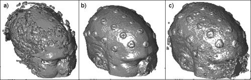
Effects of using different thresholds on surface scalp rendering obtained from MR images for one subject. (a) threshold = 0.10, TRE = 8.4 mm; (b) threshold = 0.05, TRE = 4.8 mm; (c) threshold = 0.01, TRE = 7.1 mm. Segmentation (b) shows a more appropriate surface rendition than the other two.

The MR‐derived scalp points are registered to the digitized points recorded in the functional coordinate space using the method described by Kozinska et al. [1997]1. The fitting algorithm uses a Marquardt–Levenberg optimization routine [Levenberg,1944; Marquardt,1963] applied to the case of a 3D rigid body. In brief, the algorithm minimizes the sum of squares of the distances between the two data sets. It is important to note that the distance minimized is from the data set to be transformed (i.e., the digitized points) to the closest point in the reference data set (i.e., the MR‐derived scalp surface). This may not be the actual corresponding point. Nevertheless, the algorithm offers roughly second‐order convergence by using a Taylor expansion and an iterative approach, with a varying weighted combination of an exact gradient for the first order term and an approximation to the Jacobian matrix of the partial derivatives, called the Hessian matrix, serving as the second order term. This adaptive method can help minimize the local minima problem and allows for rapid convergence, as the descent trajectory on the error function becomes less gradient‐like and more Newton–Raphson‐like near the minimum. The algorithm iterates until preset conditions are obtained (such as a predetermined number of iterations or an acceptance criterion for mean distance error) or once distance errors fail to decrease by a prespecified amount.

All data presented here used the following parameters: a 0.01‐radian angular threshold, a 0.1‐mm translational threshold, 50 maximum iterations, a weighting parameter of 2, a weighting parameter divisor of 2, and 20 maximum loop searches before the step is adjusted and a new search is started. Parameters in this range have been shown to produce good and rapid convergence for this application [Kozinska et al.,2001].

Scaling

Although the 6‐parameter rigid‐body fit reduced the bulk of the registration error, it is known that MRI gradient inhomogeneities, even in the most carefully monitored environments, can produce scaled gradient inaccuracies in the range of 1–2% (∼1–2 mm error on the scalp) in both the left‐right and anterior‐posterior dimensions [Bednarz et al.,1999; Maurer et al.,1996]. Similarly, the Polhemus® digitizer's estimates can deviate from the true value in a fashion that is in part dependent on the distance from the transmitter and in part on the presence of local magnetic field gradients (http://www.polhemus.com). Consequently, we evaluated the use of independent linear scaling factors for each of the 3 spatial dimensions (df = 3) to reduce registration errors. We applied the scaling factor after the rigid body registration, as this procedure was previously shown to results in a decrease in registration error ranging between 0.5 and 2.0 mm [Maurer et al.,1996; Schwartz et al.,1996]. Specifically, we adopted a serial approach, in which the scaling factors were estimated by performing three separate linear regressions (one for each spatial dimension) between the positions of digitized points and their closest anatomical point. This method, being based on a least‐square technique, is insensitive to the problem of local minima. In all cases the scaling factor ranged between 0.97 and 1.03.

Scaling parameters could also be estimated simultaneously with the 6‐parameters rigid body surface fitting [Koikkalainen and Lotjonen,2004]. However, this could lead to an increase in the number of local minima (associated with the increase in the number of free parameters to be estimated) and reduce the probability that the fitting algorithm will converge on the true solution [Maurer et al.,1996; Schwartz et al.,1996]. A further consideration is that previous studies support the idea that a serial approach, while yielding overall comparable fit to the original data as the simultaneous approach, provides more robust results when tested using cross‐validation methods [Maurer et al.,1996; Schwartz et al.,1996].

Scalp forcing

The scalp locations were digitized using a Polhemus® digitizer stylus. However, the stylus depression on the skin of the scalp may vary from 1 to 3 mm [Schwartz et al.,1996]. In an attempt to account for the radial digitization error thus generated, we constrained the digitized points to lie on the surface of the scalp. This “scalp forcing” was accomplished by replacing the digitized coordinates of each point (obtained after fiducial alignment, surface fitting, and scaling) with those of the closest segmented MR scalp point.

Error Estimation

In order to evaluate the various alignment methods, a measure of registration error must be used. Note that the coregistration procedure involves optimizing the fit between different data sets. As for many other optimization procedures, we need to distinguish between two ways of evaluating the goodness of the fit: (a) internal tests (in which the parameter used to estimate the error is the same used to optimize the procedure), and (b) cross‐validation tests (in which independent estimates of the error are obtained). The error estimate obtained using cross‐validation is typically considered a better estimate of the “true” error than that obtained using internal tests.

In our case, the “true” error is the map error—the error between corresponding points observed in the two modalities. However, this procedure is practically unfeasible, because it requires knowledge of which MR point corresponds to each digitized point. Of course, if this information were readily available, the coregistration procedure would consist of a simple and explicit easily‐determinable solution. Therefore, given the practical constraints outlined above, the map error is typically reserved for theoretical calculations and simulations [Fitzpatrick et al.,1998; Koikkalainen and Lotjonen,2004; Kozinska et al.,2001; Maurer et al.,1998; Singh et al.,1997]. However, an approximate estimate of the map error can be obtained using a cross‐validation approach. In the current case, this means computing the distance between estimates of the locations of corresponding points on the surface of the head obtained with digitization and MR data (after coregistration)—when these points are not used to derive the coregistration parameters. This implies using markers to make the points visible on the MR scans. We will here label this error assessment the target registration error (TRE). The TRE includes not only the map error but also other forms of error such as marker shifts between digitization and MR scanning. Therefore the TRE may be considered an upper limit for the map error.

In addition to the TRE, we will also discuss two other types of error estimates that can be (and commonly are) used to evaluate coregistration methods. The first is the fiducial registration error (FRE), defined as the distance between corresponding locations for each fiducial marker obtained after coregistration. This estimate, however, may be biased and under‐represent the map error, because fiducial information is explicitly used for coregistration. Further, it suffers from the problem of being based on a very small number of points, and therefore being potentially unstable.

The second type of error is the residual error (RE), that is, the distance between the digitized points and the closest surface points derived from the anatomical image. As minimization of this parameter is the purpose of the surface‐fitting procedure, the RE can also be biased. In fact, it is typically smaller than the map error, which may lead to overestimation of the accuracy of the coregistration procedure. A small RE does not necessarily imply a small map error. An extreme example of this occurs when the surfaces defined by the digitization and structural imaging methods are both spheres. In this case, any rotation of one of the spheres with respect to the other will produce a residual error of zero (if scaling is allowed), whereas the “truer” assessment of error, the map error, could be as large as the diameter of the sphere. However, since the RE represents the best possible fit between the two surfaces, it does represent a lower‐bound estimate of the map error, provided that the scalp data set is accurate, complete, and continuous.

It is therefore essential, if we wish to have a complete representation of the error, that we not only estimate the RE and the FRE, but also the more meaningful TRE. Having information from all three types of errors also affords the ability to compare them and form an understanding of the reliability and limitations of each—an important area for which little information is currently available.

Experimental estimation of the error

To determine registration errors and hence the efficacy of various registration strategies, 32 (16 in one case) IZI® markers were placed on the scalps of six male participants whose heads were either completely bald or shaved. Although much work on the efficacy of coregistration has been done via simulations, we consider the use of human subjects as essential to reproduce actual experimental (or clinical) conditions. Each participant provided written informed consent and the procedures used in the study were approved by the Institutional Review Board of the University of Illinois. The markers were readily visible and could be accurately located in both spaces (anatomical and functional) and served as corresponding points from which to assess the TRE and FRE. Three of the markers were on the fiducial points and were used for coregistration, whereas the remainder served solely to assess the TRE. The use of bald participants allowed for markers to be affixed directly to the scalp, thereby reducing displacement errors that were evident in preliminary work in which the markers were affixed to swim caps.

Placement of markers

Fiducial markers were placed on each participant's LPA, RPA, and nasion. The nasion was located through visual and manual inspection. The LPA and RPA were marked by means of a “T‐board” device created in our lab (see Fig. 2). This device is essentially a stencil fitted on the ear and aligned with the outer canthus of the eye. Once the device is placed, the LPA and RPA are marked in the notch of the T‐section of the board (as illustrated in Fig. 2) and are placed very near the preauricular points commonly used for EEGs/ERPs [Jasper,1958]. The use of the T‐board has proved to be more effective than visual/tactile localization of the preauricular points, which can be subject to intra‐ and inter‐experimenter error. To show the effectiveness of the T‐board, we compared the accuracy of fiducial estimations obtained on 81 subjects for whom the T‐board was used for identifying the fiducial locations with that of 147 subjects for whom the T‐board was not used. For each of these subjects we measured the FRE (fiducial registration error, see above) as a combined measure of accuracy and reliability of fiducial identification. As a reminder, this measure is based on fitting the location of the fiducial as determined using the Polhemus® digitizer to those obtained from MR recordings. In the case of these 228 subjects, these measurements were obtained in separate sessions, and therefore involved separate localizations of fiducials on the head. The FRE was, on average, 0.6 mm smaller (t(226) = 2.06, P < 0.05 one‐tailed) for the subjects for whom the T‐board was used, thus showing a significant advantage in reliability/accuracy. In addition, the use of the T‐board requires less training and less time (∼2–5 min faster per subject). Again, the emphasis on a proper choice of fiducials is not limited to the specific locations described here, but, more importantly, on the choice of points that can be repeatedly and reliably located.

Figure 2.

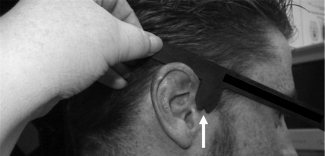
T‐board stencil used to quickly and accurately locate right (shown by white arrow) and left preauricular fiducial points.

The scalp markers were arranged in five symmetrically placed swaths of 4–7 markers running anterior to posterior (see torus‐shaped markers in Fig. 3). The markers therefore spanned most of the head and the TREs reported here represent the average over all marker locations. Markers were however omitted from the far posterior regions to ensure participant's comfort and eliminate posterior marker displacement while lying supine in the scanner.

Figure 3.

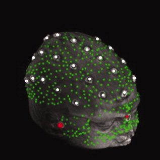
Example of digitized image coregistered with a corresponding surface MR rendition. The digitized image comprised 632 points recorded with a Polhemus® digitizer, including three fiducials (LPA, RPA and nasion IZI® markers; red dots), 29 scalp markers (torus‐shaped IZI® markers, white dots), and 600 face and scalp points (digitized green dots).

Digitization

After markers were affixed, participants were digitized with a Polhemus FastTrak® 3D digitizer (Colchester, VT; accuracy = 0.8 mm) using a recording stylus and three head‐mounted receivers (which automatically account for small movements of the head without producing position errors). The three fiducial points were digitized, followed by the scalp markers (the center of the hole in the torus markers was chosen). An additional 600 points were digitized: 400 quasi‐uniformly distributed across the head and 200 points from the face. Face points are considered extremely important for expedient and accurate surface registration. In fact, the added contour of the face improves the fitting routine because it is here that the head departs most clearly from sphericity, and therefore allows the fitting algorithm to quickly converge on unique and appropriate solutions. These points were used both for surface registration and for computation of the residual error. Examples of the digitized points from one subject, overplotted over the corresponding surface structural image, are presented in Figure 3.

MRI acquisition and marker identification

A structural MRI was recorded from each participant immediately after digitization. Scans were acquired sagitally with a T1 weighted image on a Siemens 3T scanner (TE = 4.38 ms, TR = 1800 ms, flip angle = 8°) with 144 slices, in‐plane resolution of 1.3 mm × 0.9 mm and out‐of‐plane resolution of 1.2 mm.

The IZI® markers were then identified in the MR images and their coordinates transcribed manually by the first author. To assess the reproducibility of marker identification the procedure was repeated five times on the markers of one participant. We then computed the standard deviation of the marker position on each space coordinate (x, y, and z). The average of these three standard deviations was found to be 0.74 mm. Thus, marker identification contributes less than 1 mm to the overall registration error.

RESULTS

The effects of various coregistration procedures on errors are summarized in Table I, where the means and standard deviations of the TRE, FRE, and RE are reported for different coregistration methods across the six subjects. The use of all three types of error (TRE, FRE, and RE) allows us not only to determine which registration technique is the most accurate, but also to evaluate the utility of the three types of error assessment. We consider the TRE as the most useful and unbiased estimate of map error, albeit of its upper boundary. For any given registration method, RE is in general smaller than TRE: for example, the RE of the fiducial fit was 2.8 ± 0.6 mm compared with a TRE of 8.7 ± 2.7 mm (Table I). This discrepancy in the two error measures illustrates the importance of not relying too heavily on the RE alone. The third measure of error, the FRE, was in between the other two at 3.8 ± 1.6 mm. The three measures of error for the explicit fiducial fit all differed significantly from one another (F(2,10) = 23.88, P < 0.0005), illustrating the importance of multiple means of error assessment.

Table I.

Mean errors ± SD for consecutive stages of the coregistration procedures using the moment and least‐squares method for the initial guessa

Coregistration procedure	Initial fit
	Moment	Least‐squares
Target registration error (TRE)
Initial fit	47.1 ± 4.7	8.7 ± 2.7
Surface	25.8 ± 32.6	4.9 ± 0.5
Scaling	25.1 ± 32.5	4.6 ± 0.4
Scalp forcing	25.0 ± 32.9	4.4 ± 0.6
Fiducial registration error (FRE)
Initial fit	59.8 ± 10.3	3.8 ± 1.6
Surface	24.4 ± 28.5	6.8 ± 1.9
Scaling	23.7 ± 28.1	6.7 ± 1.7
Scalp forcing	21.9 ± 26.3	5.9 ± 1.4
Residual error (RE)
Initial fit	13.2 ± 1.5	2.8 ± 0.6
Surface	3.9 ± 3.6	1.6 ± 0.1
Scaling	3.5 ± 3.4	1.4 ± 0.1
Scalp forcing	0.0 ± 0.0	0.0 ± 0.0

^aThree assessments of error are reported.

Initial Guess

Here we evaluate what is the best procedure to produce the initial “guess” to be used in the fitting procedure. Two common methods were evaluated: least‐squares fiducial fit, and moment matching. The average TRE varied widely between these methods, with the moment‐matching method yielding errors (47.1 ± 4.7 mm) that were significantly higher than the least‐squares method (8.7 ± 2.7 mm), t(5) = 13.46, P < 0.0005.

The lower performance of the moments method is likely due to the difficulty of (1) digitizing points quasi‐uniformly over the scalp such that their distribution results in similar centroids and moments compared with the MRI segmented scalp; and (2) uniquely matching ellipsoidal heads containing two axes of similar lengths (inferior‐superior and left‐right)—an effect apparent upon visualization of rendered images, whereby occasional large rotations about the anterior‐posterior axis were obvious even after surface alignment (see, for example Fig. 4). Interestingly, however, the RE for the moments method was 13.2 ± 1.5 mm, implying a reasonably good fit, and consistent with previous data reported using this method [Kozinska et al.,2001]. This suggests that the discrepancy between the two measures was the result of the ability to rotate an ellipsoidal head about certain axes without a dramatic increase in residual error.

Figure 4.

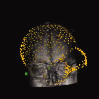
Example of misalignment associated with small RE between digitized data set and MR image from one subject, when using moments‐based alignment followed by surface fitting.

Surface Fit

Using the explicit rotation fiducial fit as a starting point for surface fitting significantly reduced the TRE (from 8.7 ± 2.7 mm to 4.9 ± 0.5 mm; t(5) = 3.75; P < 0.01 one‐tailed) compared to performing a fiducial fit alone. The RE also decreased from 2.8 to 1.6 mm (t(5) = 4.62, P < 0.005 one‐tailed). Despite the improved fitting of the TRE and RE, the FRE worsened significantly from 3.8 to 6.8 mm (t(5) = 5.34, P < 0.005 one‐tailed). This further illustrates that a high FRE does not necessarily indicate poor registration and vice versa.

When the moments‐matching technique was used as an initial guess for the surface fitting procedure, we observed an interesting phenomenon: four out of six participants converged, with an error of 5.5 ± 0.5 mm. However, two out of the six did not, with a 66.9 ± 22.3 mm error despite having similar initial errors. Furthermore, the average RE for the non‐converging participants was 8.1 mm, which could be easily misinterpreted as an acceptable fit and thus is a prime example of the local minimum problem inherent to residual‐error algorithms. This again indicates that goodness of fit based solely upon RE should be interpreted with caution. Even when we restricted the analysis to the participants who showed convergence with the moments technique, the error after moment and surface fitting was still significantly higher (0.5 mm; t(3) = 3.53, P < 0.05 one‐tailed) than that for the same participants after fiducial method and surface fitting. This implies both that within certain boundaries the surface algorithm is able to converge near the appropriate global minimum and that an advantage is still gained by an appropriate choice of initial fit.

To determine the optimal rigid‐body transform for the marker points, we applied the explicit least‐squares fit [Arun et al.,1987] to align digitized marker points to their corresponding MR marker coordinates. The FRE based upon all torus‐shaped markers being used as fiducials was 3.7 ± 0.3 mm, thus demonstrating that the fiducial fit followed by the surface registration technique converges within 1.2 mm of the rigid body limit (range = 4.9–3.7 mm). Although significant (t(5) = 5.21, P < 0.005 one‐tailed), this small error (which is on the order of marker identification precision, MRI resolution, and digitization precision) indicates the appropriateness of the Marquardt–Levenberg‐based algorithm to converge to the global minimum, given an appropriate initial condition. In sum, providing an accurate initial starting point followed by a surface fitting procedure significantly reduces registration errors.

Scaling and Scalp Forcing

To further refine the fit, we implemented two non‐rigid procedures: scaling and scalp forcing. Although each improved the data over the rigid fit on their own (scaling: 0.3 mm, t(5) = 1.94, P = 0.055 one‐tailed; forcing: 0.4 mm, t(5) = 2.04, P < 0.05 one‐tailed) the combination of the two produced the smallest error, with a TRE of 4.4 ± 0.6 mm (0.5 mm, t(5) = 2.16, P < 0.05 one‐tailed). The slight reduction in TREs using these procedures suggests that we are near the limits of resolution using cutaneous fiducials, as mentioned earlier. By contrast, the REs are not as sensitive to slight scalp displacements and therefore also show improvement upon scaling but do so in a more consistent manner (0.2 mm, t(5) = 7.25, P < 0.001 one‐tailed). The RE of the scalp forcing is not meaningful here. In fact, by definition, the RE is zero because forcing to the closest point makes each digitized point have the coordinates of one of the scalp points.

Errors attainable using the aforementioned procedures were quite small, but they were, however, significantly dependent upon a number of parameters. In the next sections we will examine some of these parameters to provide guidelines for the coregistration method.

Scalp Threshold

As mentioned previously, the scalp threshold is a parameter set by the user during the segmentation process, which varies over scans and participants. As the choice of a scalp threshold is made by the investigator, it is useful to know how it may influence the coregistration process. In fact, both the TRE and RE are dependent upon the choice of scalp threshold, as shown in Figure 5.

Figure 5.

TRE and RE dependence on scalp threshold value, obtained after fiducial and rigid body registration.

Selection of an appropriate scalp threshold that comes within a couple millimeters of the actual minimum can be done with minimal training. For instance, eight individuals were given brief (∼10 min) training on threshold selection. The mean error for optimal scalp threshold selection was 0.08 mm as measured by the difference in TRE corresponding to the threshold selected as compared to the optimal threshold.

Number of Points

The number of digitized points and the number of scalp points used for the surface fitting procedure also have a profound impact on errors (Fig. 6) as repeatedly demonstrated [Kozinska et al.,1997; Maurer et al.,1998; Noirhomme et al.,2004; Schwartz et al.,1996]. In principle, the number of digitized head points should be as many as possible. Increasing the number of points narrows the upper‐ and lower‐bound estimates (TRE and RE respectively) of the error. In practice, diminishing returns exist beyond 300 points, as the TRE function approaches an asymptote at this level. It is also important to note that, whereas the TRE decreases with the number of points (as can be expected), RE actually increases when few points are used. This is because when a very small number of points are used (say, three), it will almost always be possible to fit a surface through them with little or no error, independently on whether the fit is “real” or artifical. Only when the number of points is sufficiently large (more than 80 in our case), the real dependence of the fit on the number of points can be evaluated. Therefore, a small number of registration points give a false sense of accuracy by minimizing the RE while, in fact, the best estimate of true map error—the TRE—is quite large. These findings further bolster the claim that RE, when used in isolation, is an unreliable estimate of coregistration error.

Figure 6.

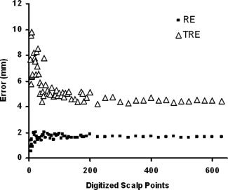
TRE and RE dependence on number of digitized points.

Error Function

A critical feature of the minimization algorithm is its robustness—the range of initial mis‐registrations from which the algorithm converges to an appropriate solution. To assess this property we used the following procedures to generate an error function for one representative subject (Subject 6): (1) We aligned the digitized data set to the MRI data set via a fiducial and surface fit and recorded TRE and RE; (2) We artificially misaligned the data set by a known amount in one dimension of translation or rotation and record TRE and RE; (3) We realigned the data set and recorded TRE and RE; (4) We repeated these procedures (steps 2–3) to systematically assess the effects over a wide range of misalignments.

The effects of initial translation and rotation misalignments on TRE and the RE both before and after realignment are shown in Figure 7. This figure only includes data from one axis of translation and one angle of rotation (the other two are not shown but produced very similar results). The figure indicates that the algorithm converges to within a few millimeters of the global minimum from a wide range of displacement values (±100 mm) and rotation angles (±50°). Also, the functions are very smooth, containing only one minimum over a wide range of starting values, providing greater confidence in the convergence.

Figure 7.

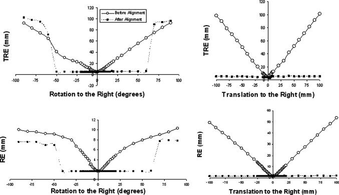
TRE and RE error functions as a result of misalignment along one translation axis and rotation angle, for one representative subject. The error estimates “before alignment” are indicated by solid lines; those “after alignment” are indicated by dashed lines.

It is important to note that whereas such plots bolster evidence for the smoothness and robustness of the error function, they are not conclusive. To obtain conclusive evidence, error information about the six‐dimensional hyper‐surface would have to be acquired. Higher dimensional error surfaces may in fact be more ‘bumpy’ revealing local troughs and may explain the local minimum entrapment we sometimes observed with the moment‐matching technique (see Fig. 4). However, such a mathematical treatment of higher order space is beyond the scope of this paper. Two‐dimensional surfaces (not shown) were plotted and, as in the unidimensional case, also reveal that the error function is smooth and contains a unique minimum.

DISCUSSION

Comparison With Published Registration Errors and Techniques

The data and techniques tested in this study deliver errors that are comparable or smaller than other established non‐invasive techniques. Although strictly limited to surgical patient studies, the most reliable and accurate technique involves bone‐implanted fiducial registration, which thus provides “gold standard” lower‐bound estimates to evaluate the accuracy of surface‐based coregistration methods. In fact, with implanted markers and under the right conditions, FREs and TREs with submillimeter precision can be achieved [Labadie et al.,2004]. It is important to note, however, that such accuracy usually involves optical digitization instrumentation, head restraints, and algorithms to precisely locate the centroids of the markers. Further, they are based on CT scans, which do not have the issues of magnetic susceptibility, gradient inhomogeneities, and chemical shift that can distort the images of fatty markers on the scalp by 1–2 mm in MR images. When a direct comparison was made on MR images, Ammirati et al. [2002] found only a small improvement in bone implanted markers as compared to skin markers (average FREs of 2.25 and 2.76 mm were obtained, respectively).

In the case of research in functional neuroimaging, we are restricted to non‐invasive procedures involving cutaneous fiducials and application of surface fitting approaches. Surface fitting is inherently a multiple non‐linear regression case, subject to the problem of local minima. This, in our case, translates in an inappropriate fitting between the recording locations obtained through digitization and the corresponding scalp points (see Fig. 3 for an example). To minimize the probability of hitting a local minimum, it is important to generate a “good” initial guess. In our study we investigated two methods for providing an initial guess: one based on a moment‐matching method and the other based on the use of fiducials.

The moment‐matching method provided REs of 13.2 and 3.9 mm before and after surface alignment, respectively, which are consistent with the 11.1–14.9 mm and 2.6–6.2 mm ranges reported by others [Kozinska et al.,2001]. However, these values contrast with large TRE in at least some of the subjects: two of the six participants had an average TRE of 66.5 mm after alignment, even though their average RE was 8.1 mm, well within the range commonly reported for these values. From this we draw two conclusions: (1) moments matching can be inaccurate and unreliable, especially if used in an automated fashion; and (2) RE is not a valid measure of registration accuracy when used in isolation.

The fiducial fit provides a better initial guess than moment matching in terms of accuracy and reliability, and can be performed reasonably quickly with no or minimal discomfort for the participant. Most commonly the fiducial fit is accomplished via skin markers or bite‐bars. A direct comparison between the two methods has been done [Adjamian et al.,2004; Singh et al.,1997], with the bite‐bar methods consistently showing smaller spreads in map error (FRE) upon repeated digitization and alignment. However, such results are expected from a rigid frame and would occur even if the bite‐bar changed position between recordings. Although Adjamian et al. [2004] have shown that the bite‐bar is displaced very little (<0.5 mm) when reinserted, no functional improvements in dipole confidence volumes for MEG median nerve stimulation were found. Additionally, bite‐bars can be uncomfortable for the participant. Reducing the spread in errors is ultimately important for alignment accuracy and reliability. Instead of accomplishing this via a bite‐bar, we chose to manufacture a stencil, the T‐board (Fig. 2), that can quickly and accurately locate LPA and RPA. A comparison of individuals coregistered with the T‐board and individuals coregistered with the old manual tactile method revealed a significant decrement in average FRE and in the standard deviation of the error. This method therefore shows promise as a reliable marking technique to reduce FRE and FRE variance while maintaining a reference frame that is affixed to the head of the subject.

In most instances where fiducial registration is used, the only error information available is the FRE. Overall, our cutaneous fiducial fit shows FREs comparable to or smaller than those reported by others [Noirhomme et al.,2004; Sinha et al.,2006].

By using more information than just a handful of fiducial markers, surface alignment can incorporate thousands of points and improve data registration. The fiducial method followed by a surface fit yielded significant improvements in TRE and RE. The REs reported were comparable to or smaller than those reported by other researchers [Huppertz et al.,1998; Kozinska et al.,2001; Lamm et al.,2001; Noirhomme et al.,2002,2004; Schwartz et al.,1996; Wang et al.,1994]. In such studies, TREs are usually confined to simulations that do not include many of the errors present with actual measures taken in a laboratory environment. However, one comparable investigation incorporated 5–6 fiducial markers for cross‐validation with surface registration in a fashion similar to our design [Brinkmann et al.,1998]. They reported map errors of 3.3–6.2 mm which are consistent with our findings.

Scaling and scalp forcing were also employed. Scaling has been shown to improve localization by 0.5–2.0 mm [Maurer et al.,1996; Schwartz et al.,1996]. Likewise, we observed a marginally significant improvement of 0.3 mm with scaling. To our knowledge, the scalp forcing technique has not been used by others. Here too, we showed a small (0.4 mm) but statistically significant improvement.

Within any registration technique, the ultimate goal is to find the set of parameters and procedures that reduce error. One such parameter is the number of scalp points. Obviously more points are better, but there is a practical tradeoff with digitization time. We find that the asymptotic limit is approached by 200–300 points (Fig. 6). Similar stability of the error function past a couple hundred points has also been shown by others [Bulan and Ozturk,2001; Kozinska et al.,1997; Maurer et al.,1998; Noirhomme et al.,2004]. Another technique that has been suggested is the deletion of outliers either before or during algorithm iterations. Although some have justified its use based on theoretical considerations alone [Kozinska et al.,2001] and others have shown reductions in RE with simulations that incorporate erroneous points [Schwartz et al.,1996], no evidence on real data sets or on TRE have been shown. When outliers were removed from our data, we found a negligible reduction in RE of 0.03 mm, and a non‐significant increase in TRE of 0.08 mm. By definition, removing outlier points as measured by closest‐point distance to the scalp surface must reduce the RE, as we in fact observed. However, note that this result does not translate to a reduction of the real mapping error (TRE). As we have already shown when discussing the effects of varying the number of points used for fitting, RE and TRE are not necessarily linked. In fact, removal of the outliers, in our case, produced a similar effect as reducing the number of points used for the surface fitting. This suggests that outlier removal may in fact increase capitalization on chance, perhaps because the points deemed to be “outliers” actually belong to the normal error distribution, and should not be eliminated. Further, the robustness analysis we reported (Fig. 7) indicates that these outliers should be of a very large magnitude to actually influence the final results in a significant manner.

Throughout this paper, we have touted the RE as being the lower‐bound estimate of the error and the TRE as the upper‐bound. Whereas this is the case in the application described here, there may be exceptions. For instance, in a scenario in which MRI scalp points are decimated causing point gaps in the surface, it is possible that the surface fit would converge on the same minimum keeping the TRE constant but causing an increase in RE. This is also theoretically possible during scalp segmentation; a scalp representation that is too deep would cause an increase in RE, and yet could still converge upon the translational and rotational minimum, causing no ill effect on the TRE. In an extreme cause, these situations could cause the RE to become larger than the TRE. We mention these scenarios here so that the idiosyncrasies between the two error measurements can be more fully appreciated and understood when interpreting coregistration accuracy.

It is common practice in studies of coregistration methods to assess registration errors by either RE or FRE. It is less common for both to be assessed together and even rarer to include a measure of the TRE. This of course is due to the practical difficulty of having multiple assessments and of computing the TRE. However, as shown in this study, only measures of TRE can provide a real estimate of registration error, and RE in particular can be misleading. Nevertheless, RE and FRE, when used in conjunction with the TRE, can give useful clues to the sources of registration error. Utilization of fiducial markers to assess map error has proven vital in ascertaining realistic metrics of registration error [Adjamian et al.,2004; Bednarz et al.,1999; Brinkmann et al.,1998; Maurer et al.,1997,1998; Noirhomme et al.,2004; Sinha et al.,2006] and further progress hinges upon continued appropriate cross‐validation techniques.

Limitations

Our error estimates were obtained under conditions which may not mirror completely those commonly used in most experimental recordings. Because it was our aim to reduce as many sources of errors as possible, fiducial markers were not replaced between the digitization and MRI sessions to minimize repositioning errors. As a consequence, the TREs presented here are likely slightly smaller than those more typically obtainable in a laboratory setting using the same procedures.

Cutaneous scalp markers placed on bald participants were a convenient method to assess TRE at multiple scalp locations, but such marker positions shift and warp on the surface of the head when in the MR scanner even when, as in our case, attempts were made to minimize such displacements. This was apparent in displacement periodicities in the swaths of rows and columns of markers distributed across the head. To prevent discomfort, no markers were placed in the far posterior regions of the head. Therefore, we have no metric of the TRE for this area. Additionally, errors reported here refer to the surface of the head and do not include possible relative changes between scalp and intracranial location, such as those due to change in decubitus, respiration, pulsation, and so on. It should be noted, though, that as we get closer to the centroid of the structure we are measuring from (in our case the head), the effects of mis‐registration should diminish, and it is likely that the center will be coregistered with a very good accuracy [Fitzpatrick et al.,1998].

Gradient inhomogeneity corrections have been shown to improve anatomical localization and registration [Bednarz et al.,1999; Jovicich et al.,2004; Maurer et al.,1996]. A 2D correction was implemented, but no improvement was noted. Computer algorithms for 3D correction [Jovicich et al.,2004,2006] were not able to be customized for our scanner and MR image acquisition sequence. It is therefore possible that such corrections could provide additional reduction in errors. Another error comes from chemical shift in the MR images, which depends in part on the type of marker used, the strength of the magnetic field, and various recording procedures. Optimization of these methods may lead to an improved TRE.

Lastly, different scanner strengths may alter the degree of accuracy obtainable using these methods. Weaker field strengths may provide a slight disadvantage at precisely recording marker locations due to poorer spatial resolution, whereas higher field strengths may distort marker locations via the chemical shift or the large local field inhomogeneity encountered near the borders of the image (i.e., air–scalp interface) as a result of the high field strength and large magnetic susceptibility differences between neighboring voxels. The use of multiple MR detectors may actually help address both of these issues.

CONCLUSION

Optimal multimodal image registration techniques are essential to accurately compare functional data sets and localize brain function to anatomy. In comparing the three‐point least‐squares fiducial method to moment‐matching techniques, the fiducial‐based approach was more precise, yielding TREs of 8.7 ± 2.7 mm. Combining a three‐point fiducial registration method followed by a surface‐matching approach and subsequent scaling and scalp forcing yielded a further reduction in TREs down to 4.4 ± 0.6 mm with REs of 1.3 ± 0.1 mm (without scalp forcing). Many parameters such as the number of digitized points, the number of scalp points, the selection of scalp thresholds, as well as the initial guess proved to be crucial in obtaining this level of accuracy. Given appropriate choices for the above parameters, the error functions were stable, robust, and smooth providing reliability and confidence to the procedures.

As we have demonstrated above, using either FRE or RE can lead to overconfidence in registration accuracy. We demonstrate multiple instances where TREs were not adequately approximated by the more commonly used REs or FREs, which raises concerns regarding the use of these error estimates in isolation. For instance, we showed that the RE can underestimate the error by several cm's in some subjects, that better fits can yield larger FREs, and that there are a number of instances in which these error estimates dissociate from each other. Hence, our data suggest that in practice RE and FRE are frequently unreliable and potentially misleading proxies for the TRE. We therefore advise using multiple error measures when assessing coregistration methods, while always including a measure of the TRE in order to properly assess the accuracy and precision of any registration procedure.

REFERENCES

- Adjamian P, Barnes GR, Hillebrand A, Holliday IE, Singh KD, Furlong PL, Harrington E, Barclay CW, Route PJG, et al. ( 2004): Co‐registration of magnetoencephalography with magnetic resonance imaging using bite‐bar fiducials and surface‐matching. Clin Neurophysiol 115: 691–698. [DOI] [PubMed] [Google Scholar]
- Ammirati M, Gross JD, Ammirati G, Dugan S ( 2002): Comparison of registration accuracy of skin‐ and bone‐implanted fiducials for frameless stereotaxis of the brain. Skull Base 12: 125–130. [DOI] [PMC free article] [PubMed] [Google Scholar]
- Arun KS, Huang TS, Blostein SD ( 1987): Least‐squares fitting of two 3‐D point sets. IEEE Trans Pattern Anal Mach Intell 9: 698–700. [DOI] [PubMed] [Google Scholar]
- Audette MA, Ferrie FP, Peters TM ( 2000): An algorithmic overview of surface registration techniques for medical imaging. Med Imaging Anal 4: 201–217. [DOI] [PubMed] [Google Scholar]
- Bednarz G, Downes MB, Corn B, Curran WJ, Goldman HW ( 1999): Evaluation of the spatial accuracy of magnetic resonance imaging‐based stereotactic target localization for gamma knife radiosurgery of functional disorders. Neurosurgery 45: 1156–1161. [DOI] [PubMed] [Google Scholar]
- Brinkmann BH, O'Brien TJ, Dresner MA, Lagerlund TD, Frank WS, Robb RA ( 1998): Scalp‐recorded EEG localization in MRI volume data. Brain Topogr 10: 245–253. [DOI] [PubMed] [Google Scholar]
- Bulan G, Ozturk C ( 2001): Comparison of two distance based alignment method in medical imaging. Proceedings of the 23rd Annual EMBS International Conference, October 25–28, Istanbul, Turkey. pp. 2606–2608.
- Crum WR, Hartkens T, Hill DLG ( 2004): Non‐rigid image registration: Theory and practice. Br J Radiol 77: 140–153. [DOI] [PubMed] [Google Scholar]
- Daisne JF, Duprez T, Weynand B, Lonneux M, Hamoir M, Reychler H, et al. ( 2004): Tumor volume in pharyngolaryngeal squamous cell carcinoma: Comparison at CT, MR imaging, and FDG PET and validation with surgical specimen. Radiology 233: 93–100. [DOI] [PubMed] [Google Scholar]
- Dogdas B, Shattuck DW, Leahy RM ( 2005): Segmentation of skull and scalp in 3‐D human MRI using mathematical morphology. Hum Brain Mapp 26: 273–285. [DOI] [PMC free article] [PubMed] [Google Scholar]
- Fitzpatrick JM, West J, Maurer CR ( 1998): Predicting error in rigid‐body, point‐based registration. IEEE Trans Med Imaging 17: 694–702. [DOI] [PubMed] [Google Scholar]
- Goldstein H ( 1950): Classical Mechanics. Reading, MA: Addison‐Wesley. [Google Scholar]
- Gratton G, Corballis P, Cho E, Fabiani M, Hood D ( 1995): Shades of gray matter: Noninvasive optical images of human brain responses during visual stimulation. Psychophysiology 32: 505–509. [DOI] [PubMed] [Google Scholar]
- Hawkes DJ ( 1998): Algorithms for radiological image registration and their clinical application. J Anat 193: 347–361. [DOI] [PMC free article] [PubMed] [Google Scholar]
- Herwig U, Satrapi P, Schonfeldt‐Lecuona C ( 2003): Using the international 10‐20 EEG system for positioning of transcranial magnetic stimulation. Brain Topogr 16: 95–99. [DOI] [PubMed] [Google Scholar]
- Hill DLG, Hawkes DJ, Gleeson MJ, Cox TCS, Strong AJ, Wong W‐L, et al. ( 1994): Accurate frameless registration of MR and CT images of the head: Applications in surgery and radiotherapy planning. Radiology 191: 447–454. [DOI] [PubMed] [Google Scholar]
- Huppertz HJ, Otte M, Grimm C, Kristeva‐Feige R, Mergner T, Lucking CH ( 1998): Estimation of the accuracy of a surface matching technique for registration of EEG and MRI data. Electroencephalogr Clin Neurophysiol 106: 409–415. [DOI] [PubMed] [Google Scholar]
- Jasper HH ( 1958): The ten‐twenty electrode system of the international federation. Clin Neurophysiol 10: 371–375. [PubMed] [Google Scholar]
- Jovicich J, Czanner S, Greve D, Haley E, Kouwe AVD, Gollub R, et al. ( 2006): Reliability in multi‐site structural MRI studies: Effects of gradient non‐linearity correction on phantom and human data. Neuroimage 30: 436–443. [DOI] [PubMed] [Google Scholar]
- Jovicich J, Haley E, Greve D, Kennedy D, Gollub R, Fischl B, et al. ( 2004): Reliability in multi‐site structural MRI studies: Effects of gradient non‐linearity correction on volume and displacement of brain subcortical structures. 10th Annual Meeting of the Organization for Human Brain Mapping, Budapest.
- Kober H, Grummisch P, Vieth J ( 1993): Precise fusion of MEG and MRI tomography using a surface fit. Biomed Eng (Berlin) 38 ( Suppl): 355–356. [Google Scholar]
- Koikkalainen J, Lotjonen J ( 2004): Reconstruction of 3‐D head geometry from digitized point sets: An evaluation study. IEEE Trans Inf Technol Biomed 8: 377–386. [DOI] [PubMed] [Google Scholar]
- Kozinska D ( 1998): Integration of EEG and MRI data of individual brain. Unpublished Dissertation, Drexel University, Imaging and Computer Vision Center. Afferent Systems Laboratory of Nencki Institute of Experimental Biology, Warsaw. University of Warsaw Interdisciplinary Center for Mathematical and Computational Modeling, Philadelphia, PA.
- Kozinska D, Carducci F, Nowinski K ( 2001): Automatic alignment of EEG/MEG and MRI data sets. Clin Neurophysiol 112: 1553–1561. [DOI] [PubMed] [Google Scholar]
- Kozinska D, Tretiak OJ, Nissanov J, Ozturk C ( 1997): Multidimensional alignment using the euclidean distance transform. Graph Models Image Process 50: 373–387. [Google Scholar]
- Labadie RF, Shah RJ, Harris SS, Cetinkaya E, Haynes DS, Fenlon MR, et al. ( 2004): Submillimetric target‐registration error using a novel, non‐invasive fiducial system for image‐guided otologic surgery. Comput Aided Surg 9: 145–153. [DOI] [PubMed] [Google Scholar]
- Lamm C, Windischberger C, Leodolter U, Moser E, Baurer H ( 2001): Co‐registration of EEG and MRI data using matching of spline interpolated and MRI‐segmented reconstructions of the scalp surface. Brain Topogr 14: 93–100. [DOI] [PubMed] [Google Scholar]
- Levenberg K ( 1944): A method for the solution of certain problems of least‐squares. Q Appl Math 2: 164–168. [Google Scholar]
- Levin DN, Pelizzari CA, Chen G, Chen C‐T, Cooper M ( 1988): Retrospective geometric correlation of MR, CT, and PET images. Radiology 169: 817–823. [DOI] [PubMed] [Google Scholar]
- Maintz JBA, Viergever MA ( 1998): A survey of medical image registration. Med Imaging Anal 2: 1–36. [DOI] [PubMed] [Google Scholar]
- Marquardt DW ( 1963): An algorithm for least‐squares estimation of nonlinear parameters. J Soc Ind Appl Math 11: 431–441. [Google Scholar]
- Maurer CR, Aboutanos GB, Dawant BM, Gadamsetty S, Margolin RA, Maciunas RJ, et al. ( 1996): Technical note. Effect of geometrical distortion correction in MR on image registration accuracy. J Comput Assist Tomogr 20: 666–679. [DOI] [PubMed] [Google Scholar]
- Maurer CR, Fitzpatrick JM, Wang MY, Galloway RL, Maciunas RJ, Allen GS ( 1997): Registration of head volume images using implantable fiducial markers. IEEE Trans Med Imaging 16: 447–462. [DOI] [PubMed] [Google Scholar]
- Maurer CR, Maciunas RJ, Fitzpatrick JM ( 1998): Registration of head CT images to physical space using a weighted combination of points and surfaces. IEEE Trans Med Imaging 17: 753–761. [DOI] [PubMed] [Google Scholar]
- Noirhomme Q, Ferrant M, Vandermeeren Y, Olivier E, Macq B, Cuisenaire O ( 2004): Registration and real‐time visualization of transcranial magnetic stimulation With 3‐D MR images. IEEE Trans Biomed Eng 51: 1994–2005. [DOI] [PubMed] [Google Scholar]
- Noirhomme Q, Romero E, Cuisenaire O, Ferrant M, Vandermeeren Y, Olivier E, et al. ( 2002): Registration of transcranial magnetic stimulation, a visualization tool for brain functions. Proceedings of DSP 14th International Conference on Digital Signal Processing, Santorini, Greece. pp. 311–314.
- Pelizzari CA, Chen GTY, Spelbring DR, Weichselbaum RR, Chen C‐T ( 1989): Accurate three‐dimensional registration of CT, PET, and/or MR images of the brain. J Comput Assist Tomogr 13: 20–26. [DOI] [PubMed] [Google Scholar]
- Powell MJD ( 1964): An efficient method for finding the minimum of a function of several variables without calculating derivatives. Comput J 7: 155–162. [Google Scholar]
- Press WH, Flannery BP, Teukolsky SA, Vetterling WT ( 1989): Numerical Recipes in C: The Art of Scientific Computing. Campbridge: Cambridge University Press. [Google Scholar]
- Schwartz D, Lemoine D, Poiseau E, Barillot C ( 1996): Registration of MEG/EEG data with 3D MRI: Methodology and precision issues. Brain Topogr 9: 101–116. [Google Scholar]
- Singh KD, Holliday IE, Furlong PL, Harding GFA ( 1997): Evaluation of MRI‐MEG/EEG co‐registration strategies using Monte Carlo simulation. Electroencephalogr Clin Neurophysiol 102: 81–85. [DOI] [PubMed] [Google Scholar]
- Sinha TK, Miga MI, Cash DM, Weil RJ ( 2006): Intraoperative cortical surface characterization using laser range scanning: Preliminary results. Oper Neurosurg 59: 368–377. [DOI] [PMC free article] [PubMed] [Google Scholar]
- Wang B, Toro C, Zeffiro TA, Hallett M ( 1994): Head surface digitization and registration: A method for mapping positions on the head onto magnetic resonance images. Brain Topogr 6: 185–192. [DOI] [PubMed] [Google Scholar]
- West J, Fitzpatrick JM, Wang MY, Darwant BM, Maurer CR, Kessler RM, et al. ( 1999): Retrospective intermodality registration techniques for images of the head: Surface‐based versus volume‐based. IEEE Trans Med Imaging 18: 144–150. [DOI] [PubMed] [Google Scholar]
- Williamson SJ, Kaufman L ( 1989): Advances in neuromagnetic instrumentation and studies of spontaneous brain activity. Brain Topogr 2: 129–139. [DOI] [PubMed] [Google Scholar]
- Williamson SJ, Lu Z‐L, Karron D, Kaufman L ( 1991): Advantages and limitations of magnetic source imaging. Brain Topogr 4: 169–180. [DOI] [PubMed] [Google Scholar]