Inference for magnitudes and delays of responses in the FIAC data using BRAINSTAT/FMRISTAT

INTRODUCTION

Our main aim is to duplicate part of the analysis of Dehaene‐Lambertz et al. [2006] (henceforth DL) so that their methods using SPM can be compared directly with ours using BRAINSTAT/FMRISTAT. To do this, we approach the Functional Image Analysis Contest (FIAC) dataset as a hierarchical study with three levels: runs, sessions, and subjects. We analyze the event sessions separately from the block sessions, but our analysis method is the same in both cases. This common analysis method seeks to detect changes in magnitude and changes in latency or delay of the responses to the stimuli, and provide standard errors for these estimates.

The changes we looked at were (1) different minus same sentence (averaged over speakers); (2) different minus same speaker (averaged over sentences); and (3) an interaction between the two. All these estimates, both of magnitudes and delays, are combined in a hierarchical mixed‐effects analysis to produce one map of voxel‐wise statistics for each of the three contrasts of scientific interest just described.

In addition to these contrasts, DL also looked at sentence effects separately for different and same speaker, and asymmetry differences between hemispheres, but only for magnitudes. Although BRAINSTAT/FMRISTAT can easily do these extra analyses, we chose to concentrate just on the two main effects of sentence and speaker and their interaction, both for magnitudes and delays.

MATERIALS AND METHODS

The details of our approach are as follows. The fMRI data were corrected for motion and different slice acquisition times using the FSL package [Smith et al., 2004]. These data were then proportionally scaled to a percentage of the whole volume mean. The data were not smoothed spatially, unlike DL, who used 8‐mm smoothing before combining the data over subjects. Separate but identical analyses were conducted for the event data and the block data.

First Level: Frames

At the first level (frames or scans), the statistical analysis of the percentages was based on a linear model with correlated errors. The design matrix of the linear model was set up in exactly the same way as in DL. For the event experiment, we constructed five variables corresponding to all sentences except the first, separately for the four conditions, and to the first sentence pooled across all conditions. For the block experiment, we constructed five variables corresponding to the second to sixth sentences in each block, separately for the four conditions, and to the first sentence pooled across all conditions. This fifth variable, which removes any effect due to the onset of the stimulus after a period of rest, was not used in any of the contrasts.

Each of the variables consisted of 1′s and 0′s for the presence/absence of each of the conditions. The five variables were then convolved with a hemodynamic response function (HRF) modeled as a difference of two gamma functions. To estimate delays, the variables for each condition were shifted over a range of delays, and a singular value decomposition was used to extract two basis functions per condition that optimally captured each shifted variable [Liao et al., 2002]. For each condition, these two basis functions, which closely match the unshifted variables and their derivatives, were added as covariates to the design matrix of the linear model, together with the fifth (“onset”) variable, giving 8 covariates for the conditions and one nuisance covariate (Fig. 1).

Figure 1.

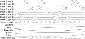
Covariates of the linear model for the first run on the first subject (block experiment). S = same, D = different, snt = sentence, spk = speaker, B = basis function. The first nine covariates model the conditions, and the remaining six model the drift. For each condition the coefficient of the first basis function is the magnitude, and the coefficient of the second basis function is used to estimate the delay shift.

Information from their coefficients was used to estimate both the magnitude of the response and the shift in its delay for each of the four conditions. An inverse tangent transformation was used, very similar to that of DL for experiment 1. The advantage of our delay estimation method is that it can be applied to any experimental design, not necessarily periodic (as in DL), and either events or blocks. Another advantage is a theoretical standard deviation (SD) for the delay as well as the magnitude, so that both magnitudes and delays can be further analyzed by the same statistical methods.

Temporal drift was removed by adding a cubic spline in the frame times to the design matrix (one covariate per 2 minutes of scan time), and spatial drift was removed by adding a covariate in the whole brain average to give 15 covariates in the design matrix (Fig. 1).

The correlation structure was modeled as an autoregressive process of degree 1. At each voxel the autocorrelation parameter was estimated from the least‐squares residuals using the Yule–Walker equations, after a bias correction for correlations induced by the linear model [Worsley et al., 2002]. The autocorrelation parameter was first regularized by 3D spatial smoothing with a Gaussian filter to control the effective degrees of freedom (DF) to at least 100 [Worsley, 2005a]. Smoothing was unnecessary for the event design since the effective DF was already greater than 100, but for the block design 2.2‐ to 2.6–mm smoothing was used to achieve ∼100 effective DF for all contrasts. The smoothed autocorrelations were used to “whiten” the data and the design matrix. The linear model was then re‐estimated using least squares on the whitened data to produce estimates of effects (contrasts) and their SDs. There were three contrasts of interest: different – same sentence, different – same speaker, and the interaction of the two (Table I).

Table I.

Contrasts used for event and block designs, and for magnitudes and delays

Contrast	Same sentence, same speaker	Same sentence, different speaker	Different sentence, same speaker	Different sentence, different speaker
Sentence	− 0.5	− 0.5	0.5	0.5
Speaker	− 0.5	0.5	− 0.5	0.5
Interaction	1	− 1	− 1	1

Second Level: Runs

The three effects in Table I, both for magnitudes and delays, together with their estimated (fixed effects) standard errors, were transformed linearly to Talairach space using a transformation estimated by the FSL package [Smith et al., 2004]. Subjects 2 and 5 were dropped due to problems with this registration (FSL needed some manual intervention that we were not aware of), leaving 14 subjects for further analysis.

The contrasts from each of the two runs per subject were combined using a fixed effects analysis for the effects (as data) with fixed effects SDs taken from the previous analysis, leaving 14 effects and their SDs for further analysis.

Third Level: Subjects

The 14 effects, one per subject, were combined using a mixed effects linear model for the effects (as data), again with SDs taken from the previous analysis. This was fitted using ReML implemented by the EM algorithm with a reparameterization to avoid positivity constraints that would bias the SD. We then estimated the ratio of the random effects variance to the fixed effects variance, then regularized this ratio by spatial smoothing with a Gaussian filter. The variance of the effect was estimated by the smoothed ratio multiplied by the fixed effects variance [Worsley et al., 2002]. The amount of smoothing was chosen to achieve 40 effective DF, and varied from 6.7–10.7 mm.

Inference

The resulting T statistic images were thresholded at P = 0.05 using the minimum given by a Bonferroni correction, random field theory, and discrete local maxima [Worsley, 2005b], taking into account the nonisotropic spatial correlation of the errors [Hayasaka et al., 2004]. Both high and low values of the T statistic images were examined. For the magnitudes, the search region was taken as the whole brain (minimum functional image > ∼6000 BOLD units, volume ∼1400 cm); for the latencies, the search region was the voxels where the T statistic image for the overall magnitude exceeded 5 (12 cm³ for the event design, 20 cm³ for the block design).

These higher‐level analyses were repeated 12 times, once for each combination of stimulus type (event or block), contrast (sentence, speaker, or interaction; see Table II), and parameter (magnitude or delay). No special code was added to BRAINSTAT to perform these calculations, apart from a script to repeat the analyses as above.

Table II.

Local maximum T statistics

	T	EF ± SD (%)	P	x, y, z	Area
Magnitude
Contrast: sentence
Experiment: event	6.57	0.86 ± 0.13	0.003	−54, −12, −20	LITG
	6.08	0.88 ± 0.14	0.015	−58, −44, −2	LMTG
	5.43	0.64 ± 0.12	0.109	−18, −64, 18	LPRE
	4.98	0.62 ± 0.12	0.426	54, −16, −14	RMTG
	−4.73	−0.48 ± 0.10	0.860	−58, −48, 34	LSmG
Experiment: block	7.61	1.00 ± 0.13	<0.001	−60, −10, −10	LMTG
	5.94	0.62 ± 0.10	0.021	56, −14, −6	RMTG
	5.69	1.17 ± 0.21	0.048	−56, −42, −2	LMTG
	−6.48	−0.58 ± 0.09	0.004	−52, −52, 46	LIPl, B40
Experiment: combination	7.85	0.96 ± 0.12	<0.001	−60, −10, −10	LMTG
	6.30	1.08 ± 0.17	0.007	−56, −42, −2	LMTG
	5.93	0.79 ± 0.13	0.022	−52, −10, −22	LITG
	5.74	0.69 ± 0.12	0.039	56, −14, −12	RMTG
	5.69	0.51 ± 0.09	0.047	60, −10, −6	RMTG
	−6.65	−0.52 ± 0.08	0.002	−52, −56, 44	LIPl
	−6.37	−0.38 ± 0.06	0.006	−50, −56, 34	LIPl
	−5.61	−0.40 ± 0.07	0.060	50, −48, 40	RIPl
Contrast: speaker
Experiment: block	5.46	0.58 ± 0.11	0.098	−64, −40, −2	LMTG, B21
Experiment: combination	5.97	0.47 ± 0.08	0.020	−64, −40, −2	LMTG, B21
Delay	5.77	0.38 ± 0.07	0.038	−58, −34, −2	LMTG
Contrast: sentence
Event	4.33	0.153 ± 0.035a	0.048	58, −18, 2	RSTG, B22

(T = EF/SD, 40 DF), P values (P ≤ 0.05, corrected), effect (EF) ± standard deviation (SD), and x, y, z Talairach coordinates (mm). Only local maxima separated by more than one FWHM (8.6 mm) are shown. Boldface indicates a local maximum inside a significant cluster (P ≤ 0.05, corrected). Combination indicates the combination of the event and block data. Only the events data were used for delay. L = Left, R = Right, I = Inferior, S = Superior, M = Middle, T = Temporal, G = Gyrus, Sm = Supramarginal, Pl = Parietal lobule, B = Brodmann. The threshold for delay local maxima is lower than that for magnitude because the delay search region is much smaller (20‐37 cm³) than the magnitude search region (1424 cm³). There were no significant activations for the interaction contrast, nor for the speaker contrast in the delays.

^aValues represent EF ± SD in seconds.

The third‐level analysis was validated by changing the sign of the effects on seven subjects chosen at random from the 14. Such an analysis should give null results. In fact, no false‐positive local maxima or clusters were detected at the P = 0.05 level on 16 such analyses of both magnitudes and delays. This gives us some assurance that the entire analysis is valid. If, on the other hand, the amount of smoothing was increased to achieve 100 effective DF, then the excessive smoothing biased the SD and resulted in too many false‐positives.

RESULTS

Efficiencies

Before we start the analysis, it is worth looking at the efficiencies of the two designs (event, block) at estimating the three contrasts in a single run. Efficiencies are just the inverse of the SD of a contrast; the lower the SD, the more efficient is the design. Of course, this depends on the underlying SD of the errors, so we measure SD relative to the SD of the errors (but for delays it depends not on the SD of the errors, but on the T statistic for the magnitude, which we fix at 5). This allows us to compare designs, and to get some idea of the sizes of effects we can hope to detect under ideal conditions.

The validity of the SDs rests on the assumptions of the linear model. In particular, they depend on the constancy of the BOLD response throughout a block. Judging by the time‐courses in DL, this seems to be a reasonable approximation, although there is some evidence of a steady decline in response after the second event in a block.

These SDs depend only on the design matrix, the contrasts, and the temporal correlation structure (AR(1) lag 1 correlation taken as 0.6) so they can be calculated before the data is collected. This is useful at the planning stage to help choose the paradigm (event or block), and parameters of the paradigm (interstimulus interval, block length) that give the smallest SD, thus making best use of the time in the scanner.

Unfortunately, it is only possible to do this at the first level in the hierarchy, that is, within subjects, since we usually have no idea in advance of the variability of an effect from one subject to another, that is, the random subject effects. In the absence of random subject effects, SDs will decrease as the square root of the number of subjects, but if random effects are present, they will add an unknown (and sometimes large) extra component of variability to the SDs that we can usually never estimate in advance of doing the experiment.

The efficiencies for a single run are shown in Figure 2 as SDs, relative to error (for magnitudes), or in seconds (for delays, assuming a T statistic for a magnitude of 5). Assuming additivity of the responses, both designs are roughly equally efficient for all contrasts in the magnitudes. For the delays the event design is much better for all contrasts. Of course, this is for a single run, and the results may differ after combining effects in higher‐level analyses, depending on the strengths of the random effects.

Figure 2.

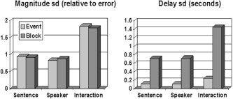
SD of designs (lower is better) for a single run, assuming additivity of responses. Interactions are harder to detect than main effects. For delays, the event design is more efficient (lower SD) than the block design; the event design estimates sentence and speaker delays to within 0.12 seconds.

Mixed Effects Analysis Over Subjects at the Third Level

To illustrate the analyses, we show in Figures 4 and 5 a display of the single subject results after level 2, and their combination in level 3. These figures are included only to show how a mixed effects analysis works, and how it combines variability both within and between subjects.

Figure 4.

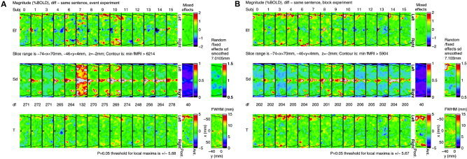
Single subject results after level 2, and their combination in level 3 for magnitudes of different – same sentence for (A) event design, and (B) block design, rotated so that left is uppermost (located on Figs. 6, 7).

Figure 5.

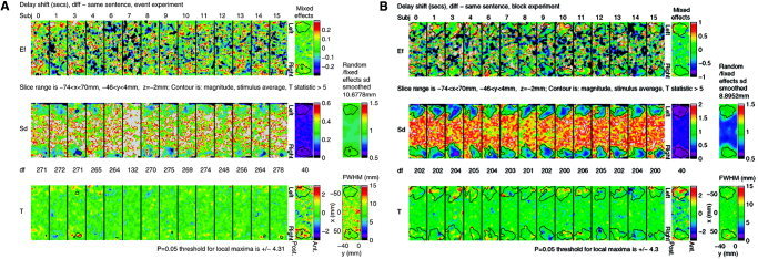
Single subject results after level 2, and their combination in level 3, for delays of different – same sentence for (A) event design, and (B) block design, rotated so that left is uppermost (located on Figs. 6, 7).

We chose just one contrast, different – same sentence, which shows the most interesting results. We show the analyses of the event and block data for both magnitude and delay. We chose part of just one slice (–74 ≤ x ≤ 70, –46 ≤ y ≤ 4, z = –2 mm), rotated 90° so that left is uppermost. This slice is located on Figures 6 and 7. The contour of the search region is added to give some idea of anatomy.

Figure 6.

Sentence and speaker magnitude T statistics (40 DF) for event superimposed on block superimposed on combined datasets, thresholded at P < 0.05 (corrected) and superimposed on the average anatomy of the 14 subjects. The portion of the slice used in Figures 4 and 5 is outlined in yellow dashes.

Figure 7.

Sentence delay T statistics (40 DF) for the event dataset, thresholded at P < 0.05 (corrected), superimposed on the search region where all conditions are activated, superimposed on the average anatomy of the 14 subjects. The portion of the slice used in Figures 4 and 5 is 4 mm below the dashed yellow outline.

The first row of each figure shows the estimated effect (EF) for each of the 14 subjects from the first two levels of the analysis (200 frames/run, 2 runs/subject). The last panel is the estimator combined over subjects using the mixed effects analysis at the third level.

The second row shows the estimated SD of the first row and their effective DF. The DFs are substantially lower than 200 × 2 = 400 due to the randomness of the estimated temporal autocorrelations [Worsley et al., 2005]. They are not quite identical since they depend on the sequencing of the stimuli, which varied from run to run.

The mixed effects SD on the right is obtained by smoothing the ratio of random/fixed effects SD by an amount chosen to give 40 effective DF [Worsley et al., 2002]. The amount of smoothing varies because it depends on the inherent smoothness of the effects (as data). The smoothed random/fixed effects SD image is shown on the far right. A value of 1 indicates that the mixed effects SD is the same as the fixed effects SD, so that the random effect is zero and can be ignored. A value greater than 1 indicates the presence of a random effect. Only magnitudes for the block design show some evidence of random effects (∼1.5), either due to different sentence effects for different subjects, or due to different locations of these effects.

The third row shows the T statistics, equal to the first row divided by the second. The P = 0.05 threshold for the final T image on the right is based on the minimum of Bonferroni, random field theory, and discrete local maxima (DLM) [Worsley, 2005b]. This requires calculation of the voxel‐wise effective full‐width at half‐maximum (FWHM), shown in the panel at the far right, which averages ∼8.6 mm. The threshold is lower for delays because the search region is much smaller (since it only makes sense to look at delays where there is some signal). The positive T statistics, particularly on the left, indicate increased magnitude and delay for different sentences over same sentences.

Comparison of Block and Event Designs

Overall, the block and event designs seem to be equally good for estimating the magnitude, but the block design has slightly lower SDs, giving slightly larger T statistics. This is not surprising, since they have roughly similar efficiencies in Figure 2. Note that the SD for the events design on Subject 7 is high (and DF low) because only one run was available.

What is surprising is the delays. Here the block design gives T statistics as high as the event design, despite the fact that the SDs are much lower (as anticipated by Fig. 2). The explanation may lie with the assumed model. Delays are estimated from both the onset and termination of the BOLD response, which is assumed to be constant throughout a block. If the response diminishes over time or terminates early, then this will result in decreased latency (see Fig. 3). It is reasonable to suppose that this might happen more for the same sentence condition (due to boredom) than with the different sentence condition (novelty will sustain interest). The time courses given by DL appear to show just this linear decline after the second event in a block, more pronounced for the same sentence condition than for the different sentence condition. The result might be an apparent increase in latency for different sentences in the blocks design due perhaps to sustained response rather than delayed response (see Fig. 3).

Figure 3.

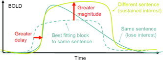
Illustration of how a decline in BOLD response during a block can alter both the apparent magnitude and delay of the block.

Can the event and block results be combined? The answer appears to be yes, at least for the magnitudes. The reason is that the magnitude effects are roughly equal between events and blocks (see also Table II). In fact, most cannot be rejected as being different by a two‐sample t test. Of course, the delays cannot be combined because of the apparent delay shifts in blocks due to a decline in BOLD response within a block, as just discussed. Accordingly, the events and blocks were combined at the second level of the hierarchy (over runs within subjects), then combined in the usual way at the third level (over subjects).

Inference

The complete results are shown in Table II for comparison with other analyses. Local maximum T statistics inside a significant cluster are indicated in bold. Clusters were thresholded at P = 0.001 (uncorrected) for magnitudes, and P = 0.01 (uncorrected) for delays. P values for clusters are based on their spatial extent measured in resels, which allows for spatially varying FWHM [Hayasaka et al., 2004]. Only the events data were used for detecting differences in delays.

There appear to be significant magnitude effects for sentence and speaker, but there is no evidence of an interaction. The sentence contrast shows both positive and negative effects. The combination of events and blocks detects more activation than either events or blocks alone, as expected, since the combined SDs are lower. There is some evidence for a sentence effect on delay for the events data, but this is not supported by a significant cluster.

Summary of Results

The most prominent effects are increases of magnitude for different – same sentence. We estimate increases as high as 1.08% ± 0.17% if events and blocks are combined. These increases are spread all along the left mid‐temporal gyrus, as reported in DL, and to a lesser extent in the right mid‐temporal gyrus (Fig. 6). There is some evidence for a decrease in magnitude in the left and right inferior parietal lobule (Brodmann area, BA, 40), although it is about half that of the increases (–0.52 ± 0.08).

There is also evidence for a speaker effect on magnitudes in roughly the same part of the left mid‐temporal gyrus as the sentence effect, BA 21. However, the size of the speaker effect is about half that of the sentence effect, peaking at 0.47 ± 0.08 for the combined data.

Turning to delays, we note again that the delay local maximum is isolated and not supported by a significant cluster. Nevertheless, there is some evidence for an increased delay of 153 ms for different sentences compared to same sentences in the right superior temporal gyrus, BA 22. What is interesting here is that the delay can be estimated so accurately, to within 35 ms.

Our conclusions can be summarized as follows:

• an increase of sentence magnitude in the left and right mid‐temporal gyri, and in the left inferior temporal gyrus;

• a smaller decrease of sentence magnitude in the left and right inferior parietal lobule, BA 40;

• a smaller increase in speaker magnitude in the left mid‐temporal gyrus, BA 21;

• an increase in sentence delay in the right superior temporal gyrus, BA 22.

DISCUSSION

Comparison with DL

We chose covariates identical to those of DL: four covariates for each condition after the first in a block or run, and one for the first event in any block or run. We analyzed exactly the same contrasts, although DL analyzed several others that we did not attempt: sentence effects under same and different speaker conditions, and tests of asymmetry.

DL also looked at delays, but for a different dataset (experiment 1) from the FIAC data analyzed here. They reported increased delay in temporal poles and inferior frontal regions, compared to Heschl's gyrus. DL was more interested in differential regional delays of the same stimulus. These differences could be partly attributed to differences in hemodynamics, rather than neuronal activity, although DL argue that hemodynamics cannot explain all the observed delay differences. On the other hand, we were looking for differential stimulus delays in the same region, which is unaffected by regional differences in hemodynamics, and so presumably only attributable to neuronal activity.

We compared our results in Table II with those reported by DL in their table 2. Overall, we found more significant activations than DL, indicating that our analysis is more sensitive, while maintaining the same false‐positive rate. This is based on the fact that none of the local maxima reported by DL reached statistical significance, whereas we found four in the same blocks dataset. DL reported only one significant cluster of 1.6 cm³, whereas we found three ranging in size from 2.7–7.9 cm³ at the same cluster threshold. Whereas DL only found evidence for an increase of sentence magnitude, we found evidence for a decrease as well. Yet this is despite that fact that we analyzed 14 subjects, whereas DL analyzed 16.

It is difficult to pinpoint which aspects of our analysis make it more sensitive. Note first that there were several nonstatistical factors that could come into play:

• different slice timing and motion correction;

• different registration;

• different smoothing (DL used 8‐mm smoothing, but we did not smooth the actual data).

There are several minor differences on the statistical side, such as the shape of the HRF, but the main ones are:

• different drift covariates;

• different strategies for dealing with temporal correlation (DL used a spatially constant temporal correlation structure, whereas ours varied spatially);

• mixed effects rather than pure random effects at the subject level;

• spatial smoothing of the random/fixed effects SD ratio to boost the effective DF from 13 to 40;

• the new DLM P values [Worsley, 2005b] that reduced the P values of local maxima by ∼43% for P values near 0.05.

These last two factors may be one of the main contributors. We ran the same analysis as in Table II but with no smoothing, so that the effective DF was 13 (as in DL) rather than 40. Significant clusters were reduced from 20 to 14, and significant local maxima were reduced from 16 to 4, with one in the blocks data. This is still more than in DL, so smoothing of the random/fixed effects SD ratio cannot be the only factor that contributes to the increased sensitivity of our analysis. We tried switching off the DLM P values, using just the best of Bonferroni and random field theory (as in DL). This increased P values by ∼10% but did not reduce the number of local maxima (switching off DLM without switching off the smoothing reduced the local maxima from 16 to 11, with 3 in the blocks data). This is still more than DL, so smoothing of the random/fixed effects SD ratio and the new DLM P values cannot be the only factors that contribute to the increased sensitivity of our analysis.

Finally, it is reassuring that the centers of activation that are reported by DL do coincide with ours.

REFERENCES

- Dehaene‐Lambertz G, Dehaene S, Anton JL, Campagne A, Ciuciu P, Dehaene GP, Denghien I, Jobert A, LeBihan D, Sigman M, Pallier C, Poline JB (2006): Functional segregation of cortical language areas by sentence repetition. Hum Brain Mapp. 27: XX–XX. [DOI] [PMC free article] [PubMed] [Google Scholar]
- Hayasaka S, Luan‐Phan K, Liberzon I, Worsley KJ, Nichols TE (2004): Non‐stationary cluster‐size inference with random field and permutation methods. Neuroimage 22: 676–687. [DOI] [PubMed] [Google Scholar]
- Liao C, Worsley KJ, Poline J‐B, Duncan GH, Evans AC (2002): Estimating the delay of the response in fMRI data. Neuroimage 16: 593–606. [DOI] [PubMed] [Google Scholar]
- Smith S, Jenkinson M, Woolrich M, Beckmann C, Behrens T, Johansen‐Berg H, Bannister P, De Luca M, Drobnjak I, Flitney D, Niazy R, Saunders J, Vickers J, Zhang Y, De Stefano N, Brady J, Matthews P (2004): Advances in functional and structural MR image analysis and implementation as FSL. Neuroimage 23: 208–219. [DOI] [PubMed] [Google Scholar]
- Taylor JE, Worsley KJ, Brett M, Cointepas Y, Hunter J, Millman J, Poline J‐B, Perez F (2005): BrainPy: an open source environment for the analysis and visualization of human brain data. Neuroimage 26: 763T‐AM. [Google Scholar]
- Worsley KJ (2005a): Spatial smoothing of autocorrelations to control the degrees of freedom in fMRI analysis. Neuroimage 26: 635–641. [DOI] [PubMed] [Google Scholar]
- Worsley KJ (2005b): An improved theoretical P‐value for SPMs based on discrete local maxima. Neuroimage 28: 1056–1062. [DOI] [PubMed] [Google Scholar]
- Worsley KJ, Liao C, Aston JAD, Petre V, Duncan GH, Morales F, Evans AC (2002): A general statistical analysis for fMRI data. Neuroimage 15: 1–15. [DOI] [PubMed] [Google Scholar]