

Abstract
A bifield stimulation method for rapidly obtaining retinotopic maps in human occipital cortex using functional MRI was compared to conventional unifield stimulation. While maintaining central fixation, each participant viewed the conventional display, consisting of a single rotating checkerboard wedge and, in a separate run, the bifield display, consisting of two symmetrically placed rotating checkerboard wedges (a ‘propeller’ configuration). Both stimulus configurations used wedges with 30 degree polar angle width, 6.8 degrees visual angle extension from fixation, and 8.3 Hz contrast polarity reversal rate. Retinotopic maps in each condition were projected onto a distortion corrected computationally flattened cortical surface representation obtained from a high‐resolution structural MRI. An automated procedure to localize borders between early visual areas revealed, as expected, that map precision increased with duration of data acquisition for both conditions. Bifield stimulation required 40% less time to yield maps with similar precision to those obtained using conventional unifield stimulation. Hum. Brain Mapping 18:22–29, 2003. © 2002 Wiley‐Liss, Inc.
Keywords: fMRI, retinotopy, mapping, vision, visual areas, striate cortex, extrastriate cortex
INTRODUCTION
Nearly a century ago, Inouye [1909] constructed a retinotopic map of human striate cortex by correlating visual field deficits with occipital lesions incurred in the 1904–1905 Russo–Japanese War [Glickstein and Fahle, 2000; see also Holmes and Lister, 1916; Holmes, 1917, 1945; Horton and Hoyt, 1991a, b]. Since then, the retinotopic organization of the primate visual system has been intensely investigated using a combination of invasive techniques (e.g., single‐cell recording and cytoarchitechtonics). However, such methods cannot be used to map human cortex if one is interested in studying the normal operation of the intact human brain.
With the advent of functional magnetic resonance imaging (fMRI), noninvasive retinotopic maps of human striate and extrastriate cortex can now be obtained [DeYoe et al., 1996; Engel et al., 1994, 1997; Sereno et al., 1995; Tootell et al., 1997]. Numerous studies have used retinotopic maps of early visual areas to study the locus of modulatory effects of perceptual and cognitive manipulations [e.g., Hadjikhani et al., 1998; Hadjikhani and Tootell, 2000; Lerner et al., 2001; Linden et al., 1999; Martinez et al., 2001; Mendola et al., 1999; Sasaki et al., 2001; Smith et al., 1998; Tootell and Hadjikhani, 2001; Tootell et al., 1998a, b; Wandell, 1999; Wandell et al., 1999]. Abnormal retinotopy due to stroke or congenital dysgenesis has been used to study cortical plasticity [Baseler et al., 1999, 2002; Goebel et al., 2001; Morland et al., 2001; Slotnick et al., 2002].
In most cases, retinotopic maps are acquired in the service of another scientific goal (e.g., “Does attention modulate cortical activity as early as area V1?”). Therefore, techniques to reduce their acquisition time are advantageous in that they allow additional time to acquire data for the primary question under investigation. Although there has been some use of multiple stimuli in retinotopic mapping [Engel et al., 1997; Tootell et al., 1995; Van Oostende et al., 1997], there has been no formal comparison with single stimulus mapping (i.e., conventional mapping). We describe a novel procedure for evaluating the precision of a given retinotopic map that was used to directly compare a multiple‐stimulus method with the conventional method.
MATERIALS AND METHODS
The most widely used method for estimating the location of borders between adjacent retintopically organized areas in early visual cortex involves the presentation of a single wedge‐shaped checkerboard pattern that reverses contrast polarity at 8 Hz and rotates about fixation at a rate of approximately 1 cycle per minute (we shall refer to this as unifield stimulation). Such stimulation produces ‘waves’ of activity in each of the early visual areas (ventrally V1, V2, VP, V4v, and dorsally V1, V2, V3, V3A, and sometimes beyond), with a reversal in the phase of the moving wave demarcating the border between adjacent areas. Either cross‐correlation or Fourier analysis can be used to estimate border locations; we used the former. The proposed procedure involves simultaneous stimulation of diametrically opposing retinal loci with two checkerboard wedges in a ‘propeller’ configuration (referred to as bifield stimulation), which reduces acquisition time by nearly half when compared to unifield stimulation.
Materials
A custom program was used to present the stimuli, acquire responses, and time‐lock the visual stimulus sequence to the fMRI data acquisition. The stimulus was back‐projected onto a screen positioned at the superior end of scanner bore. Participants were supine and viewed the stimulus through a 45‐degree angled mirror attached to the head coil such that effective viewing distance was 78 cm. Button press responses were transmitted through a fiber‐optic cable.
Images were acquired using a 1.5‐T Philips Gyroscan ACS‐NT scanner at the F.M. Kirby Research Center for Functional Brain Imaging. A receive‐only Philips end‐capped quadrature birdcage head coil was used to acquire anatomic images; a circular Philips C3 surface coil centered on the inion was used to acquire functional images.
Data analysis was conducted using BrainVoyager (Brain Innovation, Maastricht, The Netherlands). A custom program written in MATLAB (MathWorks, Natick, MA) was used to localize visual area borders.
Research protocol
Visual stimulation
Figure 1a illustrates unifield stimulation [see DeYoe et al., 1996, Engel et al., 1997; Sereno et al., 1995; Tootell et al., 1997] and Figure 1b illustrates bifield stimulation. Other than the obvious difference in stimulus configuration, i.e., one stimulus wedge vs. two stimulus wedges, all parameters were kept constant across conditions for each participant. Participants were instructed to maintain fixation throughout each run. Checkerboard wedges extended from 0.3–6.8° of visual angle from fixation and were 30° in polar angle width. The wedge reversed contrast polarity 8.3 times per second. Individual squares comprising the stimulus were scaled by the human cortical magnification factor where E2 = 0.50 and A = 22 [Slotnick et al., 2001].
Figure 1.
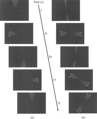
a: Snapshots of conventional unifield stimulus used for retinotopic mapping. At time = 0 sec, the entire stimulus wedge suddenly appears with its leading edge abutting the upper vertical meridian and begins to smoothly rotate counterclockwise; cycle time 72 sec. b: Snapshots of bifield stimulus. At time = 0 sec, the stimulus wedges begin to “unfold” at the upper and lower vertical meridia until they reach their full extent (at 6 sec), then smoothly rotate counterclockwise until their leading edges reach the vertical meridia where they “fold” until only the fixation point momentarily remains; cycle time 42 sec. In the time to complete one cycle using unifield stimulation, nearly two cycles are completed using bifield stimulation.
One assumption that deserves mention, most notably for bifield stimulation, is hemispheric independence. Specifically, it is assumed that right visual field stimulation activates left cortical visual areas and vice versa (i.e., strictly contralateral activation). The “unfolding” and “folding” wedges during bifield stimulation at the upper and lower vertical meridia (see Fig. 1a) were designed to isolate the stimulus to a particular hemifield; if the wedges did not collapse, there would be a period in which both wedges simultaneously stimulated each hemifield, which would result in phase uncertainty and map distortion.
A single cycle consisted of one complete revolution for unifield stimulation (requiring 72 sec) and two simultaneous half revolutions for bifield stimulation (requiring 42 sec for the entire visual field to be stimulated). The bifield cycle time was not exactly half the unifield cycle time because the unifield wedge stimulated both hemifields while traversing the vertical meridia, resulting in a relative gain of 6 sec each bifield cycle [42 = 72/2 + 6]. Each run consisted of 8 cycles resulting in a total stimulation time of 9 min 42 sec for the unifield procedure (which included 6 sec at the end of the run to complete stimulation of the right visual field) and 5 min 36 sec for the bifield procedure. Additionally, each run concluded with a 15‐sec fixation period during which the field contained only a fixation point to allow the hemodynamic response to return to baseline.
Behavioral task
To encourage vigilance and attention to the stimulus, participants were instructed to press a button with their dominant hand whenever a single randomly selected square in the stimulus flashed red for 120 msec; these target events occurred on average every 15 sec, with random temporal jitter.
fMRI data acquisition and preprocessing
After the two participants fully understood the experimental procedures and potential risks, informed consent was obtained. For each participant, a T1‐weighted scout image was acquired (8‐sec acquisition time) and subsequently used as a reference for positioning anatomic and functional images. A T1‐weighted MPRAGE (multiplanar rapidly acquired gradient echo) sequence was used for high‐resolution whole brain anatomic imaging (12‐min 24‐sec acquisition time) with 3.7 msec TE, 8‐degree flip angle, 8.1 msec TR, single excitation, coronal 256 × 256 matrix, 256 × 256 mm FOV, and 256 × 1‐mm slices with no gap (yielding 1‐mm isotropic voxels). A T2*‐weighted echo planar imaging (EPI) sequence was used to acquire functional images with 40 msec TE, 90‐degree flip angle, anterior‐to‐posterior phase encoding, 3,000 msec TR, oblique 64 × 64 matrix, 192 × 192 mm FOV, and at least 22 × 3 mm slices with no gap (yielding 3‐mm isotropic voxels). To ensure adequate sampling of functional activity associated with early visual areas, the first slice was positioned to include the occipital pole and all slices were oriented perpendicular to the calcarine sulcus.
Functional data were slice‐time corrected, motion corrected, and spatially lowpass filtered below 16 cycles/image matrix. A 3 cycles/run length temporal highpass filter was applied to the time series and the temporal lowpass filter was set to allow for a biphasic hemodynamic response. For example, in an 8‐cycle run, a 32 cycles/run length temporal lowpass filter was used (i.e., twice the Nyquist frequency).
Retinotopic mapping
For each hemifield, the 42 sec of stimulation was artificially segmented to begin at 14 distinct phases. For each phase, a hemodynamic response model with δ = 2.5 and τ = 1.25 [see Boynton et al., 1996] was cross‐correlated with the time series of every voxel. Voxels yielding a correlation above 0.20 were “painted” the color associated with the stimulus phase that resulted in maximal correlation (P < 0.01, uncorrected for multiple comparisons; see Fig. 2a). Borders of early visual areas were assumed to coincide with phase color reversals [Sereno et al., 1994].
Figure 2.
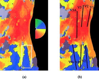
a: Left hemisphere retinotopic map corresponding to unifield stimulation of right hemifield; stimulus phase color code shown to right. Prior to flattening, inflated hemispheres were cut at the base of the calcarine sulcus, the dorsal and ventral aspects of which are represented by the top and bottom right cortical edges, respectively. White rectangle, selected region encompassing the ventral V1/V2 border used in automated border identification algorithm. b: Black lines illustrate borders between visual areas, which are labeled in black.
To aid in visualization, retinotopic maps were projected onto computationally flattened representations of the cortical surface [see Dale and Sereno, 1993; Dale et al., 1999; Drury et al., 1996; Fischl et al., 1999; Hadjikhani et al., 1998; Sereno et al., 1995; Tootell et al., 1997; Van Essen and Drury, 1997]. High‐resolution anatomic volumes were transformed into Talairach space [Talairach and Tournoux, 1988], segmented, surface reconstructed, inflated, flattened, and linear distortion corrected to less than 15% [for details, see Linden et al., 1999]. For each participant, unifield and bifield stimulation maps were then projected onto the flattened surface of the left hemisphere.
Precision metrics
A semi‐automated procedure was developed to estimate the borders between adjacent visual areas. First, a rectangular region was defined by eye that surrounded the approximate location of each border (see Fig. 2a). Phase color can equivalently be represented as phase amplitude in units of degrees (range −90 degrees to +90 degrees; corresponding to the lower and upper vertical meridian, respectively). Similar to phase color‐reversal border identification, phase amplitude valleys and peaks also represent early visual area borders.
Within the defined rectangular region, the maximum phase amplitude value in the x‐direction was selected at each 3‐mm increment in the y‐direction (where 3 mm is the distance between the center of adjacent voxels). These selected values were further refined by only including those above half the maximum value. A similar procedure was used to obtain minimum values.
To model each border, a line was fit to the selected values using the Marquardt nonlinear least‐squares algorithm [see Press et al., 1992] assuming independence in the x‐direction, such that the intercept was the point at which the line intersected the x‐axis (Fig. 2b, bottom edge). Admittedly, a linear model of visual area borders is an oversimplification; still, the model appears to be reasonable (see Fig. 3a,d) and, more importantly, model parameters can be objectively compared. Parameter values (i.e., intercepts and slopes) for all six borders per hemisphere specified a particular retinotopic map and parameters produced using unifield and bifield stimulation were directly compared.
Figure 3.
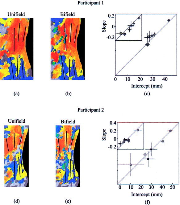
Left hemisphere retinotopic maps of two participants using unifield or bifield stimulation; borders for each map obtained independently. a: Participant 1, unifield stimulation with borders shown in black. b: Participant 1, bifield stimulation with borders shown in black. For comparative purposes, borders from unifield stimulation are also shown in white. c: Participant 1, intercepts of unifield borders on x‐axis are plotted against intercepts of bifield borders on y‐axis. Also shown to upper left, slopes of unifield borders on x‐axis are plotted against slopes of bifield borders on y‐axis. For intercept plot and slope plot, respectively, x‐axis and y‐axis scaling equivalent. Circles, V1/V2 ventral borders; triangles, V2/VP borders; squares, VP/V4v border; diamonds, V1/V2 dorsal borders; stars, V2/V3 borders; six‐point stars, V3/V3A borders. For all points, one standard error reported. Proximity to the diagonal illustrates similarity in unifield and bifield border location. d–f: Same plots for participant 2.
RESULTS
We first compared the retinotopic maps produced using the two procedures. Note that 8 cycles of unifield stimulation required ∼10 min while the same 8 cycles of bifield stimulation required ∼6 min. Figure 3 shows, with 8 cycles of stimulation, that border locations resulting from unifield and bifield stimulation were similar.
Although unifield and bifield stimulation produced maps of similar precision using 8 cycles, there was a substantial difference in acquisition duration for these two procedures. To compare map precision for several different acquisition durations, each participant's original 8 cycle datasets were truncated at the beginning and/or end to produce datasets consisting of 7, 6, 5, 4, 3, 2, and 1 cycle(s). The selection of the first cycle in a series was random with the constraint that all cycles were contiguous in time (e.g., the 6 cycle series could only begin at cycle 1, 2, or 3). For each participant, the same starting cycle for each series was used for both unifield and bifield stimulation methods to eliminate possible order effects. All 8 cycle intercepts and slopes (see Fig. 3) were assumed to estimate the “true” border locations (i.e., intercepts and slopes from V1/V2 ventral border, V2/VP border, VP/V4v border, V1/V2 dorsal border, V2/V3 border, and V3/V3A border). For each cycle length, the absolute difference between the six estimated intercepts, again using all six borders, and those of the 8‐cycle standard was measured. The mean of these intercept differences provided a global measure of deviation from the 8‐cycle standard. A similar computation was used to estimate slope deviation.
Figure 4 illustrates the results of this analysis. The mean absolute difference between the estimated border location and the standard location is plotted as a function of acquisition time. There are eight points per function, reflecting the fact that run durations lasted 1, 2, … 8 cycles. Because each cycle of unifield stimulation lasted almost twice as long as each cycle of bifield stimulation, run durations for corresponding cycle numbers increase disproportionately. By definition, border deviation was zero in the 8‐cycle run of each condition.
Figure 4.
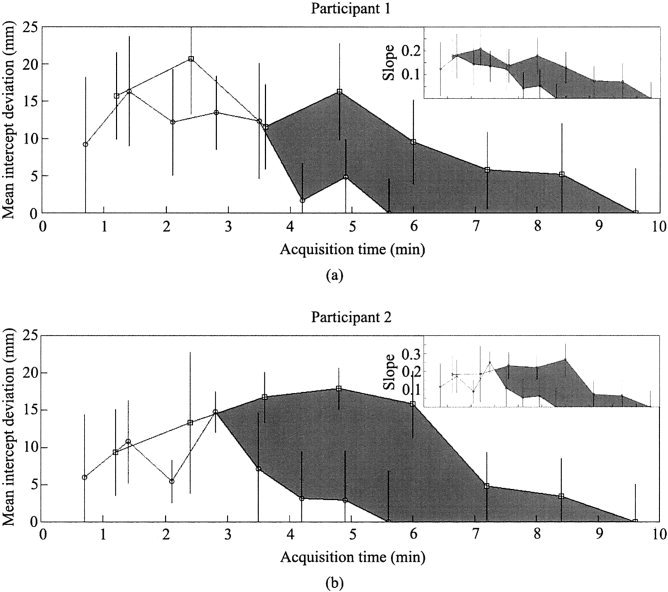
For the two participants (a,b), mean visual area border intercept deviation (of V1/V2 ventral border, V2/VP border, VP/V4v border, V1/V2 dorsal border, V2/V3 border, and V3/V3A border) as a function of acquisition time (8‐cycle map used as standard for comparison for 1‐cycle map, 2‐cycle map, 3‐cycle map, etc.). Values obtained from unifield stimulation (squares) and bifield stimulation (circles) connected to illustrate systematically better fit with longer acquisition time. Mean standard error of intercepts reported; each error obtained from Marquardt fitting algorithm. Gray region shows difference in deviation between unifield stimulation and bifield stimulation the extent of which illustrates relative superiority of bifield stimulation (i.e., smaller border deviation for a given time of acquisition). Similar plots for visual area border slope deviation are shown (top right).
The first result illustrated in Figure 4 is that the deviation scores decrease as run‐duration increases for both unifield and bifield stimulation. This is due to decreased dependence on noise with increasing number of stimulation cycles. Second, when results were dominated by signal (i.e., at acquisition times greater than 4 min), bifield stimulation always yielded smaller deviations than did unifield stimulation for the same data acquisiton duration.
DISCUSSSION
The results show that retinotopic maps obtained using the bifield stimulation approach can be acquired in approximately 40% less time than conventional mapping procedures while maintaining similar precision. Considered from the perspective of a single hemifield, the stimulus used in both methods is identical; thus, the results are not surprising. Overall, the similarity of quality to conventional retinotopic mapping methods and reduction in acquisition time indicates that the proposed method of bifield stimulation is more efficient than conventional unifield stimulation. It is important to note that the efficiency advantage reported here applies only to polar angle mapping; it does not apply to eccentricity mapping (which produces maps in the orthogonal direction).
As pointed out previously (see Visual Stimulation), the bifield stimulation method rests on the assumption that visual stimulation activates contralateral early visual areas only. For example, if visual stimulation activated both contralateral and ipsilateral early visual areas, phase uncertainty and map distortion would occur. However, the fact that retinotopic maps produced with bifield stimulation were similar to those produced with unifield stimulation, which does not rely on the contralateral activation assumption, suggests that there was no appreciable ipsilateral activation during bifield stimulation. One related caveat to consider when comparing bifield and unifield results is that the border similarity between these methods is likely restricted to the visual area boundaries discussed (i.e., the V1/V2 ventral border, V2/VP border, VP/V4v border, V1/V2 dorsal border, V2/V3 border, and V3/V3A border); Tootell et al. [1998c] have reported robust ipsilateral activation anterior to the VP/V4v border and V3/V3A border, which would be expected to distort more anterior border locations when using bifield stimulation (e.g., the V3A/V7 border). Thus, if the regions of interest include higher‐tier visual areas (e.g., V7, V8, MT, and the lateral occipital region), we suggest using unifield stimulation, rather than bifield stimulation, to avoid map distortion caused by ipsilateral activation.
Given that bifield stimulation has proven to be more efficient than unifield stimulation, the next obvious step is simultaneous stimulation in each quadrant, octant, and so on. As appealing as ad infinitum increases in efficiency may appear, a physiological upper limit necessarily exists due to hemodynamic recovery time using fMRI (which is on the order of 20 sec). Additionally, multiple stimuli in each hemifield would necessarily result in phase uncertainty.
Finally, we note that across participants and methods, at least 6 cycles of stimulation were required to produce maps of similar quality to the full 8‐cycle sequence (see Fig. 4). Six cycles of stimulation may, therefore, represent a lower bound for obtaining high‐quality retinotopic maps, at least using the methods described. Thus, using a single run consisting of 6 cycles of bifield stimulation, a high‐quality retinotopic map can be acquired in just over 4 min.
Acknowledgements
We thank Lauren Moo for insightful comments on the manuscript and Jens Schwarzbach for technical assistance. S.D.S. was supported by a training grant from the National Institutes of Health (MH19971). This work was supported by the National Institutes of Health (DA13165 to S.Y.).
REFERENCES
- Baseler HA, Morland AB, Wandell BA. 1999. Topographic organization of human visual areas in the absense of input from primary cortex. J Neurosci 19: 2619–2627. [DOI] [PMC free article] [PubMed] [Google Scholar]
- Baseler HA, Brewer AA, Sharpe LT, Morland AB, Jagle H, Wandell BA. 2002. Reorganization of human cortical maps caused by inherited photoreceptor abnormalities. Nat Neurosci 5: 364–370. [DOI] [PubMed] [Google Scholar]
- Boynton GM, Engel SA, Glover GH, Heeger DJ. 1996. Linear systems analysis of functional magnetic resonance imaging in human V1. J Neurosci 16: 4207–4221. [DOI] [PMC free article] [PubMed] [Google Scholar]
- Dale AM, Sereno MI. 1993. Improved localization of cortical activity by combining EEG and MEG with MRI cortical surface reconstruction. J Cogn Neurosci 5: 162–176. [DOI] [PubMed] [Google Scholar]
- Dale AM, Fischl B, Sereno MI. 1999. Cortical surface‐based analysis I: segmentation and surface reconstruction. Neuroimage 9: 179–194. [DOI] [PubMed] [Google Scholar]
- DeYoe EA, Carman GJ, Bandettini P, Glickman S, Wieser J, Cox R, Miller D, Neitz J. 1996. Mapping striate and extrastriate visual areas in human cerebral cortex. Proc Natl Acad Sci U S A 93: 2382–2386. [DOI] [PMC free article] [PubMed] [Google Scholar]
- Drury HA, Van Essen DC, Anderson CH, Lee CW, Coogan TA, Lewis JW. 1996. Computerized mappings of the cerebral cortex: a multiresolution flattening method and a surface‐based coordinate system. J Cogn Neurosci 8: 1–28. [DOI] [PubMed] [Google Scholar]
- Engel SA, Rumelhart DE, Wandell BA, Lee AT, Glover GH, Chichilnisky E, Shadlen MN. 1994. fMRI of human visual cortex. Nature 369: 525. [DOI] [PubMed] [Google Scholar]
- Engel SA, Glover GH, Wandell BA. 1997. Retinotopic organization in human visual cortex and the spatial precision of functional MRI. Cerebral Cortex 7: 181–192. [DOI] [PubMed] [Google Scholar]
- Fischl B, Sereno MI, Dale AM. 1999. Cortical surface‐based analysis II: inflation, flattening, and a surface based coordinate system. Neuroimage 9: 195–207. [DOI] [PubMed] [Google Scholar]
- Glickstein M, Fahle M. 2000. Visual disturbances following gunshot wounds of the cortical visual area. Oxford, UK: Oxford University Press. [Google Scholar]
- Goebel R, Muckli L, Zanella FE, Singer W, Stoerig P. 2001. Sustained extrastriate cortical activation without visual awareness revealed by fMRI studies of hemianopic patients. Vision Res 41: 1459–1474. [DOI] [PubMed] [Google Scholar]
- Hadjikhani N, Tootell RBH. 2000. Projection of rods and cones within human visual cortex. Hum Brain Mapp 9: 55–63. [DOI] [PMC free article] [PubMed] [Google Scholar]
- Hadjikhani N, Liu AK, Dale AM, Cavanagh P, Tootell RBH. 1998. Retinotopy and color selectivity in human visual cortical area V8. Nat Neurosci 1: 235–241. [DOI] [PubMed] [Google Scholar]
- Holmes G. 1917. Disturbances of vision by cerebral lesions. Br J Ophthalmol 2: 353–384. [DOI] [PMC free article] [PubMed] [Google Scholar]
- Holmes G. 1945. The organization of the visual cortex in man. Proc R Soc Lond Series B (Biol) 132: 348–361. [Google Scholar]
- Holmes G, Lister WT. 1916. Disturbances of vision from cerebral lesions with special reference to the cortical representation of the macula. Brain 39: 34–73. [PMC free article] [PubMed] [Google Scholar]
- Horton JC, Hoyt WF. 1991a. The representation of the visual field in human striate cortex. Arch Ophthalmol 109: 816–824. [DOI] [PubMed] [Google Scholar]
- Horton JC, Hoyt WF. 1991b. Quadrantic visual field defects. Brain 114: 1703–1718. [DOI] [PubMed] [Google Scholar]
- Inouye T. 1909. Die Sehstorungen bei Schussverletzungen der kortikalen Sehsphare nach Beobachtungen an Verwundeten der letzten japanischen Kriege. Leipzig: W Engelmann. [Google Scholar]
- Lerner Y, Hendler T, Ben‐Bashat D, Harel M, Malach R. 2001. A hierarchical axis of object processing stages in the human visual cortex. Cereb Cortex 11: 287–297. [DOI] [PubMed] [Google Scholar]
- Linden DEJ, Kallenbach U, Heinecke A, Singer W, Goebel R. 1999. The myth of upright vision. A psychophysical and functional imaging study of adaptation to inverting spectacles. Perception 28: 469–481. [DOI] [PubMed] [Google Scholar]
- Martinez A, DiRusso F, Anllo‐Vento L, Sereno MI, Buxton RB, Hillyard SA. 2001. Vision Res 41: 1437–1457. [DOI] [PubMed] [Google Scholar]
- Mendola JD, Dale AM, Fischl B, Liu AK, Tootell RBH. 1999. The representation of illusory and real contours in human cortical visual areas revealed by functional magnetic resonance imaging. J Neurosci 19: 8560–8572. [DOI] [PMC free article] [PubMed] [Google Scholar]
- Morland AB, Baseler HA, Hoffmann MB, Sharpe LT, Wandell BA. 2001. Abnormal retinotopic representations in human visual cortex revealed by fMRI. Acta Psychol 107: 229–247. [DOI] [PubMed] [Google Scholar]
- Press WH, Teukolsky SA, Vetterling WT, Flannery BP. 1992. Numerical recipes in C: the art of scientific computing, 2nd ed. New York: Cambridge University Press. [Google Scholar]
- Sasaki Y, Hadjikhani N, Fischl B, Liu AK, Marret S, Dale AM, Tootell RBH. 2001. Local and global attention are mapped retinotopically in human occipital cortex. Proc Natl Acad Sci U S A 98: 2077–2082. [DOI] [PMC free article] [PubMed] [Google Scholar]
- Sereno MI, McDonald CT, Allman JM. 1994. Analysis of retinotopic maps in extrastriate cortex. Cerebr Cortex 4: 601–620. [DOI] [PubMed] [Google Scholar]
- Sereno MI, Dale AM, Reppas JB, Kwong KK, Belliveau JW, Brady TJ, Rosen BR, Tootell RBH. 1995. Borders of multiple visual areas in humans revealed by functional magnetic resonance imaging. Science 268: 889–893. [DOI] [PubMed] [Google Scholar]
- Slotnick SD, Klein SA, Carney T, Sutter EE. 2001. Electrophysiological estimate of human cortical magnification. Clin Neurophysiol 112: 1349–1356. [DOI] [PubMed] [Google Scholar]
- Slotnick SD, Moo LR, Krauss G, Hart J. 2002. Large‐scale cortical displacement of a human retinotopic map. Neuroreport 13: 41–46. [DOI] [PubMed] [Google Scholar]
- Smith AT, Greenlee MW, Singh KD, Kraemer FM, Hennig J. 1998. The processing of first‐ and second‐order motion in human visual cortex assessed by functional magnetic resonance imaging (fMRI). J Neurosci 18: 3816–3830. [DOI] [PMC free article] [PubMed] [Google Scholar]
- Talairach J, Tournoux P. 1988. Co‐planar stereotaxic axis of the human brain. New York: Thieme. [Google Scholar]
- Tootell RBH, Hadjikhani N. 2001. Where is “dorsal V4” in human visual cortex? Retinotopic, topographic and functional evidence. Cereb Cortex 11: 298–311. [DOI] [PubMed] [Google Scholar]
- Tootell RBH, Reppas JB, Kwong KK, Malach R, Born RT, Brady TJ, Rosen BR, Belliveau JW. 1995. Functional analysis of human MT and related visual cortical areas using magnetic resonance imaging. J Neurosci 15: 3215–3230. [DOI] [PMC free article] [PubMed] [Google Scholar]
- Tootell RBH, Mendola JD, Hadjikhani NK, Ledden PJ, Liu AK, Reppas JB, Sereno MI, Dale AM. 1997. Functional analysis of V3A and related areas in human visual cortex. J Neurosci 17: 7060–7078. [DOI] [PMC free article] [PubMed] [Google Scholar]
- Tootell RBH, Hadjikhani NK, Vanduffel W, Liu AK, Mendola JD, Sereno MI, Dale AM. 1998a. Functional analysis of primary visual cortex (V1) in humans. Proc Natl Acad Sci U S A 95: 811–817. [DOI] [PMC free article] [PubMed] [Google Scholar]
- Tootell RBH, Hadjikhani N, Hall EK, Marrett S, Vanduffel W, Vaughan JT, Dale AM. 1998b. The retinotopy of visual spatial attention. Neuron 21: 1409–1422. [DOI] [PubMed] [Google Scholar]
- Tootell RBH, Mendola JD, Hadjikhani NK, Liu AK, Dale AM. 1998c. The representation of the ipsilateral visual field in human cerebral cortex. Proc Natl Acad Sci U S A 95: 818–824. [DOI] [PMC free article] [PubMed] [Google Scholar]
- Van Essen DC, Drury HA. 1997. Structural and functional analysis of human cerebral cortex using a surface‐based atlas. J Neurosci 17: 7079–7102. [DOI] [PMC free article] [PubMed] [Google Scholar]
- Van Oostende S, Sunaert S, Van Hecke P, Marchal G, Orban GA. 1997. The kinetic occipital (KO) region in man: an fMRI study. Cerebral Cortex 7: 690–701. [DOI] [PubMed] [Google Scholar]
- Wandell BA. 1999. Computational neuroimaging of human visual cortex. Annu Rev Neurosci 22: 145–173. [DOI] [PubMed] [Google Scholar]
- Wandell BA, Poirson AB, Newsome WT, Baseler HA, Boynton GM, Huk A, Gandhi S, Sharpe LT. 1999. Color signals in human motion‐selective cortex. Neuron 24: 901–909. [DOI] [PubMed] [Google Scholar]