Abstract
Translating recent advances in abdominal aortic aneurysm (AAA) growth and remodeling (G&R) knowledge into a predictive, patient-specific clinical treatment tool requires a major paradigm shift in computational modelling. The objectives of this study are to develop a prediction framework that 1) first calibrates the physical AAA G&R model using patient-specific serial computed tomography (CT) scan images, 2) predicts the expansion of an AAA in the future, and 3) quantifies the associated uncertainty in the prediction. We adopt a Bayesian calibration method to calibrate parameters in the G&R computational model and predict the magnitude of AAA expansion. The proposed Bayesian approach can take different sources of uncertainty; therefore, it is well suited to achieve our aims in predicting the AAA expansion process as well as in computing the propagated uncertainty. We demonstrate how to achieve the proposed aims by solving the formulated Bayesian calibration problems for cases with the synthetic G&R model output data and real medical patient-specific CT data. We compare and discuss the performance of predictions and computation time under different sampling cases of the model output data and patient data, both of which are simulated by the G&R computation. Furthermore, we apply our Bayesian calibration to real patient-specific serial CT data and validate our prediction. The accuracy and efficiency of the proposed method is promising, which appeals to computational and medical communities.
I. Introduction
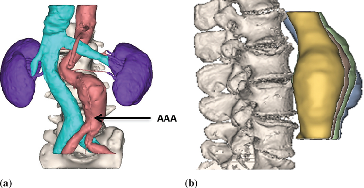
An abdominal aortic aneurysm (AAA) is an enlarged localized volume in the lower part of the aorta, which supplies blood to a large part of the body (see Fig. 1). Enlargement of the aorta by more than 50% of its normal diameter is defined as an aortic aneurysm. The vast majority (over 90%) of aortic aneurysms occur in the abdominal region, specifically the infrarenal aorta [1]. In general, an aorta with a diameter larger than 3 cm is considered an aneurysm.
Fig. 1.
AAA location and serial CT images. (a) The location of an AAA is indicated by an arrow, while the cyan color coated region on the left indicates the inferior vena cava vein. (b) Four serial AAA CT images 1, 2, 3, and 4. Information on registration of CT scan images can be found in [27].
A ruptured aneurysm can cause life threatening internal bleeding. If ruptured, patient mortality rates are greater than 80% [2]. Depending on the size and rate of growth, treatment of an AAA may vary from watchful waiting to emergency surgery. Once an AAA is found, doctors will closely monitor the AAA so that surgery can be planned if it becomes necessary. Since either open or endovascular repair (EVAR) of small AAAs (< 5.5 cm) can result in peri-operative deaths (4.4% with open repair and 1.0% with EVAR) [3], performing unnecessary surgeries increases patient risk. A thorough understanding of the expansion and rupture of AAAs is thus needed in order to minimize unnecessary patient risk. While significant advances have been made in the management of AAA patients [4], this disease still carries a high mortality rate. During the last decade, bio-chemo-mechanical studies have been integrating computational modeling with increased understanding of the expansion and weakening of aneurysms, [5], [6], [7], [8]. Recently, this computational platform, called a growth and remodeling (G&R) model, has been developed and incorporated with patient-specific anatomical information, which aids in treatment planning on a per-patient basis [9], [10]. Those models developed the G&R model to take into account both elastic degeneration and stress-mediated collagen turnover during AAA development using finite element analysis (FEA). The G&R models were validated through using human aortic mechanical tests that characterize material properties and serial image data of one patient (both non-aneurysmal and aneurysmal aortas) [9] [11]. A coupled simulation of G&R with hemodynamics was conducted for studying its effects on AAA expansion [12], [13]. Geometric, kinetic and material parameters for AAA expansion can help to predict intrasac-pressure dependent vascular adaptation after endovascular repair [14], [15]. A patient-specific distribution of aortic wall properties has been investigated from open surgery and ultrasound imaging [16], [17]. Recently, a phenomenological model (without bio-chemo-mechanical considerations) has been proposed to predict AAA shapes and their quantified uncertainties [18].
Translating recent computational advances into a predictive tool for individualized clinical treatment, however, requires a major paradigm shift due to the incompleteness of the G&R model, limited information, and uncertainty associated with clinical measurements with regard to each individual patient. In this study, with a small set of real follow-up image data from patients, we develop a computational-statistical method to predict AAA expansion utilizing a simple initial elastin damage and a set of selected internal key parameters of a G&R model. Most importantly, the associated uncertainty in the prediction propagated from various sources of uncertainty, needs to be correctly quantified. For example, the G&R model’s internal parameters need to be carefully adjusted according to patient-specific data, e.g., serial computed tomography (CT) images, in order to make better prediction and so be useful for clinical decisions. The aims of this paper are to develop a framework that 1) first calibrates the physical AAA G&R model using patient-specific serial CT scan images, 2) predicts the expansion of an AAA in the future, and 3) quantifies the associated uncertainty in the prediction. To achieve our aims, we perform Bayesian calibration [19] of our computational AAA G&R model. In particular, Bayesian calibration will be used to incorporate the computational G&R model, patient-specific data (e.g., CT scan images), and various uncertainties as well as to compute the uncertainty level of the prediction on the AAA expansion. In other words, the measurement from the patient was utilized to “calibrate” parameters in the G&R computational model and to update the prediction of AAA expansion. There are growing interests in patient-specific modeling [20]–[22] and in applying Bayesian calibration. The use of patient-specific models using Gaussian process regression can outperform population-based models for vital-sign forecasting using time series of patient vital signs [22].
To the best of our knowledge, we are the first to apply the Bayesian calibration method to the AAA G&R computational model. We aim to make the G&R computational model viable to aid clinicians in decision making. Hawkins-Daarud et al. [23] used a Bayesian framework to address questions on validation, model selection, and uncertainty quantification for tumor growth. Biehler et al. [24] presents an uncertainty quantification framework based on multi-fidelity sampling and Bayesian formulations and analyzes the impact of the uncertainty in the input parameter on mechanical quantities typically related to abdominal aortic aneurysm rupture potential. In contrast to discrete model candidates for model selection in [23], we consider a statistical model for the true physical process by introducing two Gaussian random fields [25] for the G&R computational model and the inadequacy of the model. We adopt a Bayesian calibration technique proposed in [19] to calibrate parameters in the G&R computational model and predict the AAA expansion.
The contributions of our paper are as follows. First, we formulate the Bayesian calibration of our AAA G&R computational model taking into account model inadequacy, prior distributions of model parameters [26], measurement errors, and most importantly, patient-specific serial CT scan images. Next, we demonstrate how to achieve the proposed aims by solving the formulated Bayesian calibration problem using a simulation study and real data analysis. In particular, we compare and discuss the performance and computation time under different sampling cases for the computational model output data and (synthesized) patient data, both of which are synthesized by the G&R computation. We apply our Bayesian calibration to the real patient-specific CT data and validate our prediction, showing the effectiveness of our approach to the computational science and medical communities in aiding decision making.
The organization of the paper is as follows. Section II introduces the AAA G&R model, the quantity of interest in making prediction, and the full statistical model with hyperparameters for Bayesian calibration. In Section III, we discuss assumptions for priors and then provide the posterior and predictive distributions under the Bayesian framework. Section IV describes the design of the in silico simulation study with synthetic observation data and a case study with real patient data. In Section V, we present the results of the Bayesian calibration for both simulation and real data cases. Finally, we provide some discussions and concluding remarks in Section VI. In what follows, we introduce all the G&R and statistical models needed in our Bayesian calibration.
II. Methods
A. AAA G&R computational model
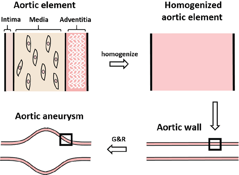
The Bayesian calibration framework includes a computational G&R model of AAA as a data input, where the detailed computational G&R model was described in Zeinali-Davarani et al. [28]. Our computational G&R model has three parts: constitutive relations of intrinsic material behavior, a stress-mediated production function, and a damage function. To describe material behavior, we assume that the aorta is comprised of three stress-bearing constituents, viz. elastin, collagen fiber families, and vasoactive smooth muscle cells. The G&R model then uses a constrained mixture approach that homogenizes the three structural constituents and simulates AAA expansion by a finite element method. The constrained mixture approach is described in Fig. 2.
Fig. 2.
The constrained mixture approach is illustrated for three main constituents of aortic wall, elastin, collagen and smooth muscle cells for modeling AAA growth. The G&R model is implemented in a 2D finite element method (FEM) and computationally generates an AAA from an initial healthy aorta to its growth by prescribing a elastin damage profile and by utilizing the stress-mediated G&R at every FEM elements [33].
Each constituent, in addition to its contribution to the construction and strength of the artery’s wall, has its own individual properties. The population-based material parameter distributions of abdominal aortas obtained from ex vivo tests of human tissues [29] was given by Seyedsalehi et al. [26]. The stress-mediated production functions connect the stress-state of the artery to changes of the mass rates with a stress-mediated feedback approach. Moreover, in the G&R model, the AAA is initialized by imposing damage function to the elastin of normal aorta. The initialization is supported by the previous study [30], which shows that one of the main features of AAA is the elastin reduction. The study [11] elaborates that the degradation of elastin can directly form patient-specific shapes of aneurysms. On the other hand, the other factors, such as alteration of intrinsic material parameters [16], disturbed collagen production [31] and hemodynamics [32], are taken as the minor reason of initialization of AAA, and are considered as modeling errors in our approach.
The damage function takes into account elastin and vasoactive smooth muscle, therein elastin plays a key role in the mechanical behavior of aorta. Elastin contributes resilience and elasticity to the aortic tissue; but when the person’s age is advanced, elastin cannot be replaced. For an AAA, the localized dilation of the aorta is initiated by the degradation of the elastin. This degradation will reduce the amount of elastin, leading to the weakening of the wall. The damage will result in the increase of the diameter and wall stress of the aneurysm. The increase of the stress in constituents results in an increase in the accumulation of collagen and smooth muscles as a way to compensate for the elastin’s loss and decrease stress in the wall. All the relations and details of the model have been previously reported by Zeinali-Davarani et al. [34] and Kwon et al. [14]. In the current study, we decided to use the 2D axisymmetric G&R model for our Bayesian calibration. As discussed, the elastin damage in the aortic wall initiates the growth of the aneurysm. Here we define the initial elastin’s damage function as
| (1) |
where s is the coordinate defined on the centerline. g(s) = 1− d(s) is the ratio of remaining elastin to the initial amount at s. The damage function in (1) contains two parameters of interest {θ1,θ2} to be calibrated from the real data and another quantity α that is identified via CT images without Bayesian calibration. They have their own specific effects on the shape of the damage function and thus on the stress-stretch and geometrical state of the AAA at a given time.
In particular, θ1 is a scaling factor with θ1 ∈ [0,1). An increase in θ1 toward 1 will increase the degradation of elastin and thus increase the dilatation of the artery. θ1 = 0 means no degradation; hence, the artery will retain its initial state. α corresponds to the location on the centerline at which the maximum damage occurs, so it is relatively easy to be estimated from the CT images compared to θ1 and θ2. In particular, the location of the maximum diameter would be approximately close to the location of the maximum damage; hence, we estimated α by finding the location of the maximum diameter using the CT images. The modeling errors due to α-approximation will be considered as our model inadequacy, which will be a part of the statistical model in our Bayesian calibration. Thus, we fix α on an appropriate value obtained from CT images directly a-priori and focus on calibration of θ1 and θ2 in a Bayesian way.
B. Quantity of interest (QoI) for AAA G&R
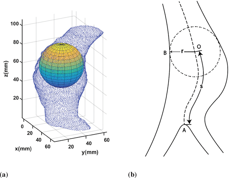
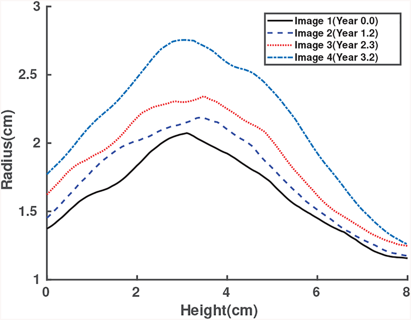
The quantity of interest (QoI) of AAA G&R is what we want to predict in AAA growth in the future. The selection of the QoI will let us subsequently determine the statistical models and investigate the associated uncertainties. In this study, we truncate patient’s scan images into the sections that range from the aortic bifurcation point to the lower renal branch. For each section, a centerline is generated by the maximally inscribed sphere method in the AAA 3D images [35]. The radii of the inscribed spheres r, which are selected as the QoI, are given at the axial position (or height) along the centerline s and at the time t. Figs. 3a and 3b show inscribed spheres and the resulting centerline, respectively, for a given 3D point cloud sampled from CT scan image data from a patient. This QoI selection is consistent with medical practice in which the diameter of the AAA is used as an important decision variable [2], [36]. To align serial geometries of the same patient, we assume that QoIs with the same height correspond to the same point on the aorta, albeit scanned at the different time. Fig. 4 shows the QoIs of Patient 1 prepared for the Bayesian calibration procedure, from scan images of Patient 1 taken at 4 time points in series. Bayesian calibration combines the QoIs and the simulation data to calibrate the selected parameters in the computational model. In this paper we consider the following questions: Can we predict the radius vs. height profiles for CT scan images 3 and 4 in the future given CT scan images 1 and 2 in Fig. 4? What is the uncertainty associated with such prediction? The answers to the those questions using the proposed Bayesian calibration method for this particular patient-specific data set shown in Fig. 4, are given in Section V-B as a part of the real data study case.
Fig. 3.
Inscribed spheres and center lines. (a) An inscribed sphere with point clouds from the CT scan images. (b) A center line generated by inscribed spheres.
Fig. 4.
Radius vs height coordinate on the centerline measured from CT scans of Patient 1 over the surveillance period. The lines from bottom to top represent images 1, 2, 3, and 4, respectively.
C. Calibration model
Let ζ(x) be the QoI of the true AAA G&R process, the input variable of which is denoted by x and defined as x = [t s], where t is the time and s is the height coordinate on the centerline as illustrated in Fig. 3b. Suppose that we have n observations. To model possible observation error, e.g., resolution and segmentation errors in CT scan images, we consider the noisy observations as follows.
| (2) |
where the measurement error, i.e., the difference between the observation and the true process is denoted by εi. We further assume that each εi is independent and identically distributed (i.i.d.) as . We denote the QoI of the G&R computational model output at x as r(x,θ), where θ is called a set of calibration parameters, or calibration inputs. In the G&R computational model for the AAA expansion, damage parameters serve as calibration parameters that are patient specific for the AAA growth, i.e., the calibration parameters are θ = [θ1 θ2] defined in Section II-A.
Given the available QoI of the G&R computational model, we model the true process as
| (3) |
where δ(·) is a model inadequacy function, i.e., model error, which is independent of the computational outputs. It is natural to assume the true AAA expansion process ζ(x) cannot be fully described by the computational model, therefore we introduce δ(x) to represent the discrepancy in (3).
By combining (2) and (3), we have
| (4) |
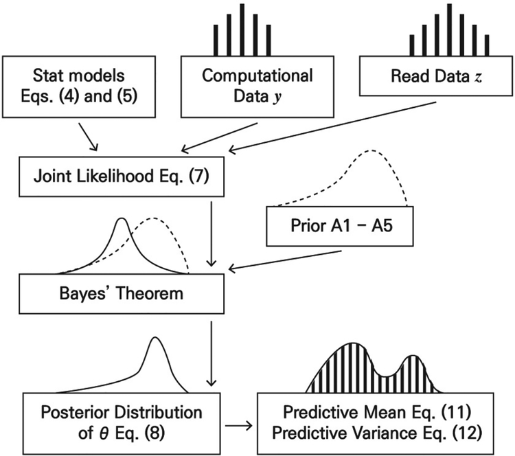
which gives a calibration model that relates G&R computational outputs with the true process and the observations. The Bayesian calibration method [19] we adopt in this paper introduces Gaussian process priors for the computational model and the model error in order to calibrate θ and predict the QoI. Fig. 5 shows the flow-chart for Bayesian calibration. The regular Bayesian analysis just includes one data source as its input. Our Bayesian calibration model integrates two data sources (i.e., computational data and real CT image data as shown in Fig. 5) to implement predictions. The statistical models in Fig. 5 are further assumed to follow Gaussian processes, which will be discussed in the next section.
Fig. 5.
The flow-chart of Bayesian calibration. Statistical models (4) and (5) are combined by computational data y and real data z to produce the joint likelihood. The posterior distribution of θ in (8) can then be used to predictive mean (11) and predictive variance (12) of the QoI.
D. Statistical models
Let be the Gaussian process (GP) with the mean function m(·) and the covariance function k(·, ·). A GP is flexible and popularly used as a prior model for functional prediction [37], [38]. We introduce GPs as prior beliefs for the G&R computational model and the model inadequacy, respectively by
| (5) |
Gaussian processes combine the flexibility of being able to model arbitrary smooth functions, with the simplicity of a Bayesian specification that only requires inference over a small number of hyperparameters [37]–[40]. The QoI for AAA G&R is a simple bell curve shape as in Fig. 4. Following the theoretical rationale [40], we used a mixture of 3 Gaussian processes (computational model, model inadequacy, and observational error) to model the QoI. We believe that our application (i.e., simple curve shape) is well suited for the assumptions and our corresponding model, QoI, and measurement errors can be realizable from the Gaussian processes in (5). One can make a distributional assumption other than Gaussian to be more flexible, but performance can be hindered by computational complexity.
We use a linear combination of basis functions to form a general mean structure. Hence for (5), we have and , where ()T is the transpose operator. The mean function of the model error m2 is linear in time t and location s. The coefficients β = [β1 β2] are hyperparameters in a Bayesian context.
The covariance functions use the squared exponential functions as follows.
where is the weighted norm of (x − x′) by Ω. Weights of Ωx, Ωθ and are all diagonal matrices. ψ = [ψ1 ψ2]denotes the hyperparameters with
| (6) |
where vec(Ω) vectorizes the diagonal entries of Ω. ψ1 contains hyperparameters of r(·, ·) in (5). ψ2 contains hyperparameters of δ(·) in (5). Note that k1 is a multiplicative kernel. The correlation is large when is small.
III. Bayesian Analysis For Calibration
This section outlines our Bayesian approach. More technical details can be found in the supplement of this paper.
A. Joint likelihood
We define as calibration inputs and x* as variable inputs of the computational model. Let N be the total number of pairs of variable and calibration inputs. We further define the computational model output vector (Fig. 5) as and the corresponding input matrix as
The Gaussian process prior on the computational model then gives .
Let n be the number of real observations and be the set of real observations (Fig. 5) corresponding to the variable input matrix . To calibrate θ from the observations, we augment variable inputs Xo with θ such that Xo(θ) = [(x1,θ)T,⋯,(xn,θ)T]T. From the calibration model, we then have
where In is the n×n identity matrix.
We combine the computational model outputs and observations, , which we call a data vector.
| (7) |
B. Calibration
To estimate (θ,β,λ,ψ) under the Bayesian framework, we consider the following prior distributions and assumptions.
A.1 β1 and β2 have non-informative priors, i.e., p(β1,β2) ∝ 1.
A.2 θ is independent of the other parameters.
A.3 θ follows a normal distribution.
A.4 ψ1 and ψ2 in (6) follow lognormal distributions.
A.5 log(λ) has a non-informative prior, i.e., p(log(λ)) ∝ 1.
Note that based on A.1 and A.2, we obtain the joint prior distribution in the following form p(θ,β,λ,ψ) ∝ p(θ)p(λ)p(ψ). For A.3, we use the sample mean and variance of the calibration parameter inputs that were used to generate computational model outputs for the normal prior density. A.4 guarantees that ψ1 and ψ2 in (6) are positive values in the calculation since they are all hyperparameters in covariance functions. Together with the prior specification given above, the full joint posterior distribution of θ,β,λ,ψ given d, i.e., p(θ,β,λ,ψ | d) can be found. In this form, β is integrated out easily, while λ and ψ are estimated by maximizing conditional posterior distributions p(ψ1 |y) and p(λ,ψ2 |d,ψ1), as proposed by Kennedy and O’Hagan (2001) [19]. Having estimated λ and ψ and plugging them into p(θ | λ,ψ,d), we obtain the posterior distribution of the calibration parameter θ to be
| (8) |
C. Prediction
We introduce variable inputs to be used for prediction. The corresponding prediction of the QoI at given variable inputs Xp is denoted as . For quality of the prediction, we can consider variable inputs in Xc that cover Xp.
Under the Bayesian framework, a prediction can be made using the predictive distribution of the (unobserved) true process ζ(x) given full data d. First we obtain the distribution of ζ(·) conditional on θ, and , which is also normal. Therefore, its mean function is given by
| (9) |
Additionally, its covariance function can be found
| (10) |
We can then obtain the predictive distribution of ζ(x) given d, and by integrating θ out from with respect to the posterior distribution of θ given in (8). From (9) and (10), we obtain the predictive expectation and variance of ζ(·) evaluated at inputs Xp as follows (Fig. 5):
| (11) |
and
| (12) |
where ζ(Xp) = [ζ(xn+1) ⋯ ζ(xn+m)]T. We then obtain the prediction and its variance using the Markov Chain Monte Carlo (MCMC) technique (see more details in the supplemental document).
IV. Data
We consider two studies. In the in silico study case, we use the G&R computational model of the AAA expansion to generate synthetic observations in addition to producing computational model outputs. In this case, we know the realized true process along with the parameters that generate it for validation. In the second case, we use real data sets, i.e., observations from three sets of patient specific CT scan images. The G&R computational model is used only to obtain computational model outputs in this real-world data study. When implementing Bayesian analysis, we standardize all the inputs x, θ and outputs y, z to stabilize computation.
A. In silico simulated study
For our in silico study, we generate r(x,θ) from the G&R computational model. To validate our approach, we realize and set patient specific values on the calibration parameters (say θ0) for the synthesized true process so that we evaluate the estimated calibration parameters. Recall that for the damage function, we need to set θ1, θ2, α to produce the G&R computational model outputs. For the simulated observation case, we set θ1 = 0.65, θ2 = 6 and α = 3.1. Thus, we have θ0 = [0.65 6] for the true process. For the variable inputs x = [t s], we consider 8 equally spaced s from 0 to 9 cm and a time step of 5 days, which are fixed throughout the study. The time duration is 7 years, but several different choices of sampling times are considered. Note that when we implement Bayesian calibration, the values of the QoI (the radius with respect to the centerline) are standardized as well so that its mean is 0 and its variance is 1.
Once we obtain a realization of r(x,θ0), we add model and observation errors to get the final observations. The model error, δ(x), is realized from the model assumption (5) with β2 = [0.001 0.001], ω21 = 1, ω22 = 1, and . Then the standard deviation of model error δ(x) on each height at each time is about {0.071, 0.032}. The observation error ε is generated from with λ = 0.001, i.e., . The standard deviation of standardized computational outputs r is 1. To generate simulated observations, we add a model error process of 7.1% or 3.2% (with respect to r) and an observation error process of 3.2%. We chose these values for the model and observation errors in order to produce a data set that best illustrates the effects of different noise levels and sampling schemes.
We also need computational model outputs at various combinations of variable inputs and calibration inputs. For calibration inputs, we consider θ = [θ1 θ2] ∈ {0.5,0.65,0.8} × {2,6,10} so that there are total 9 combinations of θ1 and θ2. For variable inputs, s will be considered at 8 equally spaced values from 0 to 15 cm. For time t, we consider three different scenarios to see the effects of different time resolutions. With two choices of , there are a total of 6 different scenarios. Table I gives the label of each scenario. Further details of each scenario are given in Table II. With three cases of sampling time grids and the two levels of , we want to investigate the behavior of interaction between the computational model and Bayesian calibration. In Case 1, computational model inputs have a sparse time grid while those in Case 3 have a denser one. In Case 2, the computational model inputs do not cover the full time range we want to predict while those in Case 1 and Case 3 do.
TABLE I.
Differences in Xc and for simulation cases
| sampling time in Xc | ||
|---|---|---|
| every 2 years | Case 1a | Case 1b |
| every 1.5 years | Case 2a | Case 2b/2c |
| every 1 year | Case 3a | Case 3b |
TABLE II.
Parameters for case studies
| Case 1b | Case 2b/2c | Case 3b | Real Data | ||||
|---|---|---|---|---|---|---|---|
| Xc dimension | 288 × 4 | 360 × 4 | 576 × 4 | 288 × 4 | |||
| Xo dimension | 56 × 2 | 72 × 2 | 16 × 2 | ||||
| Xp dimension | 48 × 2 | 48 × 2 | 16 × 2 | ||||
| y dimension | 288 × 1 | 360 × 1 | 576 × 1 | 288 × 1 | |||
| z dimension | 56 × 1 | 72 × 1 | 16 × 1 | ||||
| δ % of r | 7.2% | 3.2% | 7.2% | 3.2% | 7.2% | 3.2% | 10% |
We note that variable inputs and calibration inputs for the proposed Bayesian calibration are standardized in the actual implementation so that we can assume the realized calibration inputs are centered at zero. We then use 0.3 as prior means of θ1 and θ2 (away from the zero) to investigate the robustness of prior distributions. In addition, we consider 0.1 for prior variances of θ1 and θ2. The same setting for the prior of θ1 and θ2 is used later in the real observation case. Note that the normal prior can be used for θ1 that is constrained to the interval [0,1]. As θ1 was standardized (mean is 0, standard deviation is 1), the range of θ1 becomes [−1.3,1.3] based on the parameter values we use. We set the prior of mean at 0.3, and the variance of prior at 0.1 (standard deviation is 0.32). According to the empirical rule, 99.7% of the samples from the prior will lie in the interval [−0.66,1.26] which contains in the interval [−1.3,1.3].
B. Real observation case
For the real observation case, we consider 4 serial CT scan images of Patient 1 as shown in Fig. 1. This particular patient’s CT scan examination spans a period of 3 years. For each image, we measured the corresponding radius (QoI) at each height on the centerline as illustrated in Fig. 4 using the maximally-inscribed sphere method developed in [35]. From the preliminary study of the damage shape with respect to the CT scan images, we selected α = 3.1 for (1) a-priori.
In addition, we selected the reasonable range of the calibration parameter θ a-priori to produce comparable computational model outputs for the particular observations (Fig. 4). More specifically, as prior information to determine the range of the calibration parameter θ, we fit the diameter of the computational model outputs to the diameter calculated from CT scan images using fminsearch in MATLAB (Mathwork, Natick, USA) and found the optimum value to be [θ1 θ2] = [0.2 0.9]. From this information, we consider θ = [θ1 θ2] ∈ {0.05,0.2,0.35} × {0.7,0.90,0.99}. For these 9 combinations of θ, we run the G&R model to produce the computational model outputs. More details for this real observation case are given in Table II. Aforementioned are for the set-ups of patient 1. We follow the same scheme to generate observations from 4 serial CT scan images of patients 2 and 3. For patient 2, we found α = 1.9 and we assumed that θ = [θ1 θ2] ∈ {0.055,0.065,0.075} × {0.65,0.75,0.85}. For patient 3, we found α = 1.3 and we assumed that θ = [θ1 θ2] ∈ {0.265,0.305,0.345} × {1.75,2.05,2.35}.
V. Results
In this section, we present results of the Bayesian calibration method on simulated observations and real observations as described in Section IV.
For simulated observations, means and standard deviations of relative errors across locations at different times are provided in Table IV. We gauge relative errors R = [R1⋯Rm]T over the height of the AAA that are calculated as
| (13) |
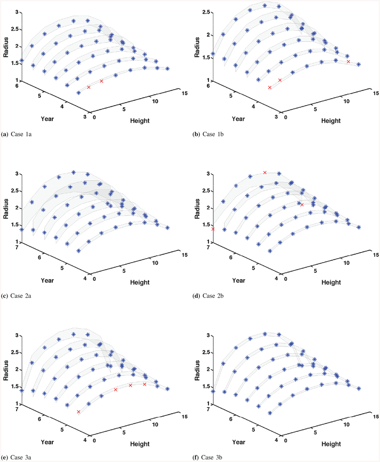
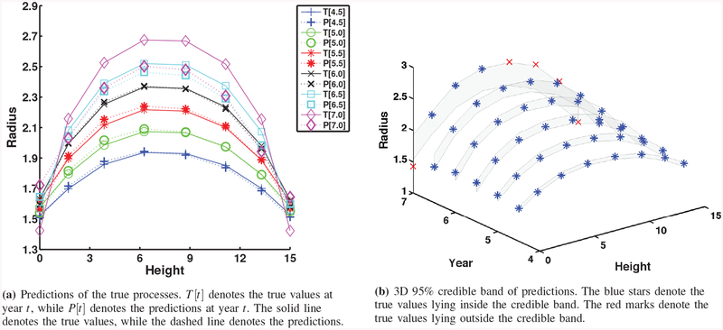
where T = [T1 ⋯ Tm]T is the realized true process for the simulated observation case that is described in Section IV-A. Correspondingly, 95% credible bands with true processes are presented in Fig. 6.
TABLE IV.
Means and standard deviations of relative errors across locations at different years in simulated observation cases. In each cell of the table, the former is the mean value and the latter is the standard deviation.
| Year | Case 1a | Case 1b | Year | Case 2a | Case 2b | Case 3a | Case 3b |
|---|---|---|---|---|---|---|---|
| 3.5 | 0.0116 / 0.0095 | 0.0133 / 0.0080 | 4.5 | 0.0247 / 0.0205 | 0.0032 / 0.0021 | 0.0199 / 0.0103 | 0.0058 / 0.0032 |
| 4.0 | 0.0116 / 0.0095 | 0.0105 / 0.0077 | 5.0 | 0.0325 / 0.0277 | 0.0088 / 0.0039 | 0.0176 / 0.0090 | 0.0038 / 0.0025 |
| 4.5 | 0.0171 / 0.0119 | 0.0137 / 0.0102 | 5.5 | 0.0367 / 0.0380 | 0.0140 / 0.0066 | 0.0144 / 0.0077 | 0.0039 / 0.0024 |
| 5.0 | 0.0239 / 0.0141 | 0.0220 / 0.0115 | 6.0 | 0.0376 / 0.0331 | 0.0071 / 0.0069 | 0.0144 / 0.0076 | 0.0056 / 0.0049 |
| 5.5 | 0.0251 / 0.0155 | 0.0237 / 0.0104 | 6.5 | 0.0343 / 0.0168 | 0.0271 / 0.0168 | 0.0194 / 0.0066 | 0.0096 / 0.0073 |
| 6.0 | 0.0211 / 0.0086 | 0.0099 / 0.0063 | 7.0 | 0.0970 / 0.0334 | 0.0965 / 0.0628 | 0.0213 / 0.0082 | 0.0090 / 0.0090 |
Fig. 6.
3D 95% credible band of predictions. The blue stars denote the true values lying inside the credible band. The red marks denote the true values lying outside the credible band.
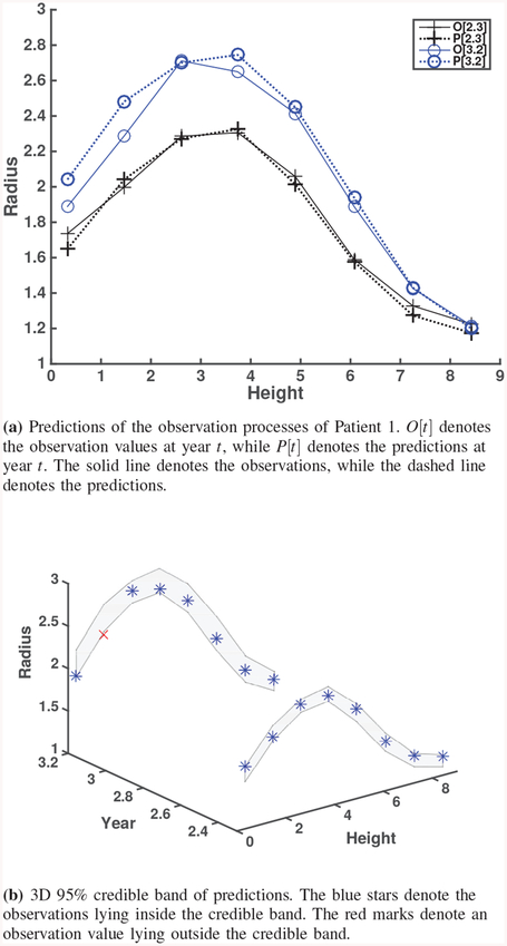
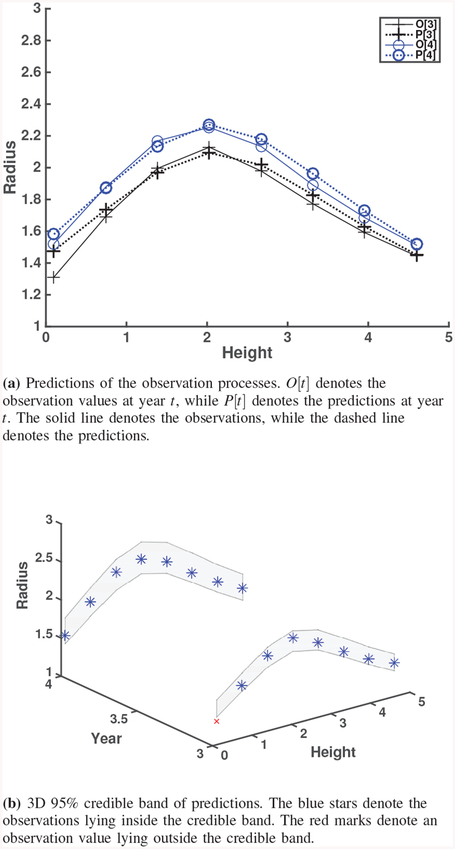
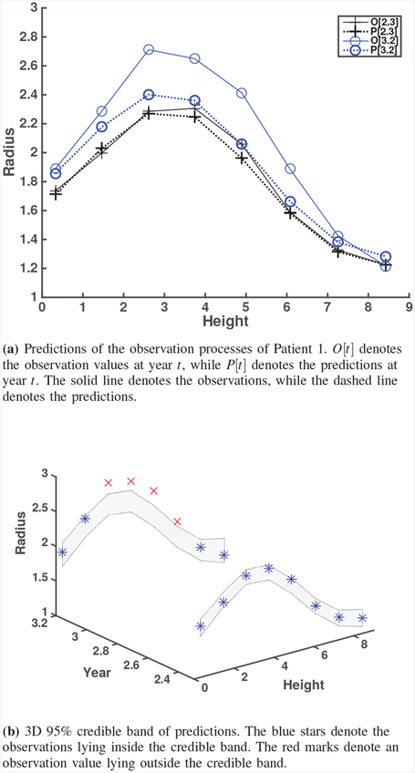
For the real observations, the prediction and credible band graphs are given together in Fig. 8, Fig. 10 and Fig. 11. Since only observations are available for these cases, relative errors for prediction are calculated by replacing {Ti} in (13) with the observations (i.e., noisy true values).
Fig. 8.
Predictions and credible bands for Real observation of Patient 1.
Fig. 10.
Predictions and credible bands for Real observation of Patient 2.
Fig. 11.
Predictions and credible bands for Real observation of Patient 3.
A. Results from simulated observation cases
In AAA clinical management, typically physicians use maximum diameters in cm and classify AAA patients by the maximum diameter. Therefore, we provided the predicted maximum diameter and its prediction error (i.e., prediction minus observation) in Table III. Among all the cases, the result of Case 3b outperforms all the others as it gives the smallest prediction error. Besides, we calculated log predictive likelihood for different cases. Compared with Case 1 and Case 3, Case 2 did not have G&R model information at years 6.5 or later to predict at years 6.5 and 7. Therefore, the log predictive likelihood of Case 2 is much smaller than the other two cases. The result is consistent with our findings that Case 2 has the lowest prediction performance.
TABLE III.
Predicted maximum diameter and prediction error at different years in simulated observation cases. In each cell of the table, the former is the maximum diameter (cm) and the latter is the prediction error.
| Year | Case 1a | Case 1b | Year | Case 2a | Case 2b | Case 3a | Case 3b |
|---|---|---|---|---|---|---|---|
| 3.5 | 3.3712 / 0.0154 | 3.3694 / −0.0057 | 4.5 | 3.8760 / −0.0169 | 3.8716 / −0.0183 | 3.9102 / 0.0795 | 3.8460 / −0.0255 |
| 4.0 | 3.6258 / 0.0269 | 3.6318 / 0.0108 | 5.0 | 4.1844 / −0.0061 | 4.1740 / 0.0170 | 4.1816 / 0.0772 | 4.1142 / −0.0195 |
| 4.5 | 3.9222 / 0.0638 | 3.9330 / 0.0558 | 5.5 | 4.4886 / 0.0014 | 4.4704 / 0.0439 | 4.4650 / 0.0766 | 4.3930 / −0.0115 |
| 5.0 | 4.2362 / 0.1062 | 4.2450 / 0.1012 | 6.0 | 4.7412 / −0.0399 | 4.7162 / 0.0140 | 4.7658 / 0.0838 | 4.6898 / 0.0025 |
| 5.5 | 4.5256 / 0.1124 | 4.5332 / 0.1130 | 6.5 | 4.9026 / −0.1654 | 4.8992 / −0.0916 | 5.0830 / 0.1004 | 5.0040 / 0.0184 |
| 6.0 | 4.7690 / 0.0585 | 4.7616 / 0.0565 | 7.0 | 4.9586 / −0.4012 | 4.9956 / −0.3038 | 5.3910 / 0.1023 | 5.3074 / 0.0043 |
| Log predictive likelihood | −215.6521 | −188.9377 | −987.0728 | −1563.825 | −87.39966 | −108.842 |
Relative errors in (13) (Table IV) are used for scientists and engineers to perform analytical comparison of prediction performance. From Table IV and Fig. 6 of the simulation study, we observe the following findings. Prediction quality improves when more computational model outputs are used for calibration. When we consider different sampling time resolutions, prediction quality monotonically improves from Case 1 (coarse resolution) to Case 3 (fine resolution). Smaller model errors (Cases 1b, 2b, and 3b) provide better prediction results. Compared to Cases 1a, 2a, and 3a, prediction quality from Cases 1b, 2b, and 3b is better. As one can expect, prediction quality decreases at the year for which the computational model outputs or observations are not available for calibration. For example, at years 4.5, 5, and 5.5, the errors between the true processes and predictions are more pronounced in Case 1a since both computational model outputs and observations are not available at those years. In particular, predictions at years 6.5 and 7 for Case 2 are the worst in terms of relative errors. Such results are reflected in wide credible bands as well. A possible reason is that calibration for Case 2 did not have information at years 6.5 or later to predict at years 6.5 and 7. Recall that computational model outputs are up to year 6 and observations are up to year 4. On the other hand, calibration for Case 1 has computational model outputs at year 6 to predict at years 4.5, 5 and 5.5. This result suggests that we can use computational model outputs at future times during calibration for better prediction. In this regard, results from Case 3 are better than Cases 1 and 2. However, more computational model outputs in the calibration process implies higher computational burden.
From the Bayesian calibration, we have posterior samples of calibration parameters as well as hyperparameters. For the simulated observation case, true values of parameters (values that were used to generated the data are actually close to the prior mean) are known so that we can compare the performance of Bayesian calibration for various simulation scenarios. The priors and posteriors (calibrated estimates) of θ1 and θ2 for each case are provided in Table V. Corresponding figures of comparison between priors and posteriors are shown in the supplemental document.
TABLE V.
Prior and posterior distributions of θ1 and θ2
| Case | (mean, std1) | (mean, std) | (mean, std) | (mean, std) |
|---|---|---|---|---|
| 1a | (0.678,0.035) | (6.050,0.105) | (0.686,0.010) | (6.052,0.003) |
| 1b | (0.668,0.023) | (5.912,0.147) | (0.671,0.007) | (5.908,0.007) |
| 2a | (0.681,0.035) | (6.072,0.105) | (0.690,0.003) | (6.074,0.003) |
| 2b | (0.672,0.024) | (6.013,0.080) | (0.676,0.005) | (6.013,0.002) |
| 3a | (0.669,0.016) | (5.997,0.056) | (0.672,0.002) | (5.997,9 · 10−4) |
| 3b | (0.660,0.010) | (6.003,0.040) | (0.661,8 · 10−4) | (6.003,5 · 10−4) |
| 2c | (0.665,0.032) | (5.992,0.115) | (0.669,0.008) | (5.992,0.004) |
| Patient 1 | (0.250,0.096) | (0.858,0.062) | (0.322,0.090) | (1.147,0.508) |
| Patient 2 | (0.065,0.008) | (0.750,0.082) | (0.070,0.005) | (0.716,0.053) |
| Patient 3 | (0.305,0.033) | (2.050,0.245) | (0.308,0.027) | (1.882,0.105) |
std denotes the standard deviation.
and denote priors of θ1 and θ2.
and denote posteriors of θ1 and θ2.
Comparing the posteriors of θ1 and θ2 in all cases, we clearly notice that the posteriors of Case 3 have the sharpest peaks around the true values, which can be utilized as point estimators. As shown in Table V, the posterior estimates of θ1 and θ2 in Case 3b are the closest to their true values among all cases. This also illustrates that more information from computational model outputs can give more accurate estimates of the calibrated parameters. Consequently, better estimation of calibrated parameters is likely to give us better quality of predictions.
Robustness to prior selection:
To investigate the impact of different priors on Bayesian calibration, we compare the results of Case 2b and Case 2c, where Case 2c is the same as Case 2b except the prior variances of calibration parameters are 10 times larger.
The posteriors of θ1 and θ2 for Case 2c cover the prior mean values, but they have larger posterior variances than those from Case 2b due to the larger prior variances. We see that the 95% credible bands (Figs. 6d and 7b) are similar even though their prior variances are quite different. This can be seen also in the predictions and relative errors (e.g., supplemental document). This implies that our Bayesian calibration method is robust to such changes in priors. Therefore, we may use a diffuse prior that can cover all the possible values of parameters θ by learning the statistical information from the background and the computational model. One can choose the priors for the real observation case in a similar way.
Fig. 7.
Predictions and credible bands for Case 2c.
B. Results from real observation case
In this section, we discuss the calibration results from real observations of patient 1 using CT images 1–4 as shown in Fig. 4, i.e., CT images taken at 0, 1.2, 2.3, and 3.2 years, respectively. To generate computational model outputs to be used for calibration, we consider the inputs Xc for a computational model as follows. Eight heights uniformly ranging from 0 to 8.2 are chosen. For calibration parameter, θ1 is chosen from {0.05,0.2,0.35} and θ2 is chosen from {0.7,0.90,0.99}. The computation takes 30 minutes. The G&R computation has been coded and implemented using MATLAB R2012a on an Intel Core i7 3770 3.4 GHz Processor with 12 GB of RAM. Table V shows the estimates of all calibration parameters. The prior means of θ1 and θ2 are 0.25 and 0.858, and their prior standard deviations are 0.96 and 0.062, respectively. The resulting posterior means of θ1 and θ2 from Bayesian analysis are 0.322, and 1.147, and their standard deviations are 0.09 and 0.508, respectively.
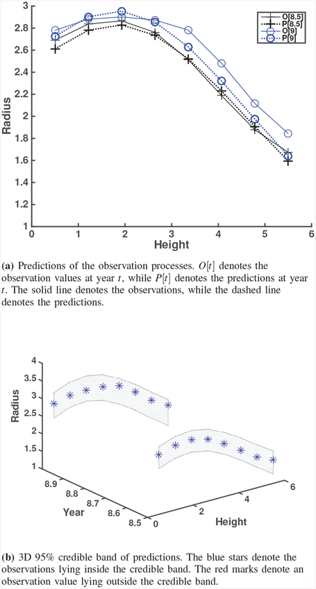
We withhold observations for the last two years during the calibration procedure in order to validate our approach by comparing predictions on the last two years (CT images 3 and 4, taken at 2.3 and 3.2 years, respectively). In contrast to the simulation study, we compare the results with observations (noisy true values) since the true process is not available in the real observations. The difference between the true process and the observation (the measurement error) is estimated to be from the real observation data used for Bayesian calibration as shown in Table II. There are some larger discrepancies in the lower part of predictions at 3.2 years, which can be shown in terms of relative errors. Most of the relative errors are less than 5%. Besides, Fig. 8a shows how close the Bayesian calibration model predicts the observation (i.e., noisy true) values. From Fig. 8b, we also find that only one observation value lies outside of the credible bands. These results support that our approach has a capability to predict AAA expansion using real data.
C. Comparison with a baseline model
We performed Gaussian process (GP) regression as a baseline model to demonstrate the effectiveness of our proposed approach. This baseline model was trained and performed using GPML package [41] in MATLAB 2018. The covariance was set as an ARD squared exponential covariance (i.e., covSEard). The results are presented in Tables VI and VII, and Figs. 8 and 9. Our Bayesian calibration outperforms GP prediction in terms of prediction errors (Table VI) as well as relative errors (Table VII), especially in a long time prediction horizon. This is due to the fact that GP prediction does not take into account the G&R model, therefore, it does not have predictive capability in the future time horizon. In addition, our Bayesian calibration updates calibration parameters of the G&R model in Table V and other uncertainties (Fig. 5), while GP prediction neglects them. In results, under GP prediction, credible bands are not predicted precisely as shown in Fig. 9(b). More comparisons against GP prediction are given in the supplemental document.
TABLE VI.
Predicted maximum diameter and prediction error at different years in real observation cases. In each cell of the table, the former is the maximum diameter (cm) and the latter is the prediction error (cm).
| Method | Years | Patient 1 | Years | Patient 2 | Years | Patient 3 |
|---|---|---|---|---|---|---|
| 3.2 | 5.4902 / 0.0678 | 4.0 | 4.5415 / 0.0696 | 9.0 | 5.9070 / 0.2095 | |
| 3.2 | 4.8029 / −1.2390 | 4.0 | 4.3127 / −0.3880 | 9.0 | 5.6185 / −0.3676 |
TABLE VII.
Means and standard deviations of relative errors across locations at different years in real observation cases. In each cell of the table, the former is the mean value and the latter is the standard deviation.
| Method | Years | Patient 1 | Years | Patient 2 | Years | Patient 3 |
|---|---|---|---|---|---|---|
| 3.2 | 0.0329 / 0.0326 | 4.0 | 0.0197 / 0.0137 | 9.0 | 0.0435 / 0.0367 | |
| 3.2 | 0.0802 / 0.0479 | 4.0 | 0.0494 / 0.0136 | 9.0 | 0.0548 / 0.0205 |
Fig. 9.
GP Predictions and credible bands for Real observation of Patient 1.
D. Insights from three real data cases
To get more insights from multiple patient cases, we also run our model on patients 2 and 3 (Table VI and Table VII). Both patients 1 and 2 have better prediction performance than patient 3 (Figs. 8, 10 and 11). In particular, for patient 3, the growth (to the right of the maximal point) is much faster, which may be due to the longer time horizon (8.5 and 9 years) as compared to patients 1 and 2. Our Bayesian calibration method accommodates this phenomenon appropriately. The credible bands of patient 3 are wider as well predicted (Fig. 11). In the elastin’s degradation function, an increase in θ1 will inflate the damage, thus accelerate the growth of aneurysm. θ2 controls the area under degradation, so an increase in θ2 will increase the area of aneurysm. As shown in Table V, patient 2 has the smallest posterior mean values, i.e., predictions (θ1,θ2) = (0.07,0.716) while patient 3 has the largest values (0.308 and 1.882), which matches well with that AAA enlargement of patient 3 increases with a larger magnitude and the AAA of patient 2 increases with a smaller magnitude. This trend can be seen in Figs. 10 and 11. Our Bayesian calibration takes into account this growth scheme and uncertainties. For other results of patients 2 and 3, please see the supplemental document.
VI. Discussion And Conclusion
From prediction graphs of Case 3 in the supplement document, we notice that the diameters of proximal and distal ends of the true line at year 7 tend to be smaller than the previous ones. When the AAA is gradually expanding, the end of both regions can be axially compressed, which means the radii of the two ends are often contracted. The computational model successfully captures this phenomenon. Currently we are studying serial images of abdominal aortic aneurysms, registered with the vertebral column. We speculate that the renal vein and artery, superior mesenteric artery, and iliac bifurcation can serve as an anchor (both serial and circumferential directions at the superior and inferior boundaries) to the infrarenal AAA during expansion. Hence, it may be possible that the physical constraints of the tethering of those vessels provide a strong confinement, or an anchor at the region of the aorta. During the AAA expansion, the volume of the AAA’s sac will gradually increase while stretching mostly in the circumferential direction and slightly in the axial direction simultaneously. Hence, because of the AAA expansion and the confinement in axial direction, the neck and distal part of aorta (from renal branches to the AAA’s sac) will be compressed in the axial direction. Using the 3D growth and remodeling simulation, Zeinali et al. (2012) [10] show the local change in the stress distribution, in which the stress of the sac is increased but the neck’s stress is decreased.
Recall that we estimated α a-priori before Bayesian calibration since we assume that the peak location of the future AAA and its overall geometry do not change significantly from the previous scans. As illustrated in the real observation case, the AAA peak location and the aneurysm shape did not significantly change during the follow-up images, which support our approach.
Estimates of β11 (the coefficient for time t) are always positive, which means the radii of AAAs increase in time due to AAA expansion. Estimates of β12 (the coefficient for θ1) are also positive in all cases, which means the QoI, i.e., the radii of AAA increases as θ1 increases. This can be explained by the damage function (1). The QoI increases while the elastin contents decreases as the amplitude of the damage function (e.g., θ1) increases. Estimates of β13 (the coefficient for θ2) are negative in the Patient 1 case while all β13’s are positive in the simulation cases. This could be due to the fact that θ2 values are largely different between real and simulation observations. On the other hand, the estimates of β21, β22 and in all cases are small. This implies that the computational model could explain most of the linear and covariance structures of the true process.
The results from the simulation case study suggest that Bayesian calibration may be used to combine the computational model, prior and uncertainty models, and real observations to predict the QoI at future times or at unobserved locations. The computational model output data provide a deterministic trend of the expansion process, which is modeled by a Gaussian process. Additionally, computational model discrepancies obtained from real observations are modeled by another Gaussian process. When we have more information from the computational model (in the form of finer grids for inputs Xc), we achieve lower prediction errors, and the posteriors of parameters θ1 and θ2 are more likely to concentrate on their true values as illustrated in our simulation results. We also find that posteriors and predictions from our approach are robust to the selection of priors for θ1 and θ2. In the real observation case of one patient, the results of Bayesian calibration indicated that the predictions are reasonably good when compared with the unused last two observations. Most of the unused observations match reasonably well with predictions and lie inside the 95% credible bands. The model and the observation errors collectively capture the structure of the true process in a consistent manner from a Bayesian perspective.
From our various case studies, we believe that our Bayesian calibration process has high capability of predicting complex G&R AAA processes. As compared with GP prediction with a set of real serial observations, we show that our Bayesian calibration outperforms GP prediction in prediction capability. This demonstrates that the additional complexity of Bayesian calibration is warranted by improved performance over a less complex method. We also analyze the results of our Bayesian calibration on three real data cases and show an insightful trend on calibrated model parameters. However, there is a need for validating our approach with a large number of real observation cases to evaluate its performance and efficacy in a clinical sense. We believe that for given past CT images of a patient, Bayesian calibration can help to guide the scheduling of future CT scans according to predictions with the credible bands.
A. Limitations
Limitations exist in our G&R simulations. First, one time initial damage of elastin in the focal lesion is considered to be over-simplified and compound effects (e.g., local hemodynamics, intraluminal thrombus, and axial or bending stretch) are not taken into the AAA growth mechanism. Second, values of material parameters were chosen by using only population-based values (Seyedsalehi et al. [26]) in contrast to those of patient-specific. Finally, there are various sources of errors in identifying axial location and diameter measurements from image segmentation, 3D reconstruction and registration processes (e.g., the smoothing effects, alignment of centerlines at different time points) that might affect the performance of the Bayesian calibration. Despite of the various limitations, our current study with multiple of real data sets showed promising results of Bayesian calibration compared to a naive GP prediction since our approach takes into account both the computational G&R model and its model inadequacy (5) along with various uncertainties. With better understanding of various compound effects on damage and remodeling mechanism, the Bayesian calibration will be further improved to be a reliable clinical tool in future.
B. Future work
As future work, we plan to consider complicated damage functional shapes with more parameters as well as asymmetric AAA expansion in a 3D space. We plan to investigate how to deal with high-dimensional calibration parameters when various compound effects and complex functions are used for damage and the rate of mass production. Finally, we will investigate how to incorporate other available patient-specific data for Bayesian calibration of a particular patient case.
Supplementary Material
Acknowledgment
Authors gratefully acknowledge the support, in part, by the National Heart, Lung, and Blood Institute of the National Institutes of Health (R01HL115185 and R21HL113857) and National Science Foundation (CMMI-1150376). The contents are solely the responsibility of the authors and do not necessarily represent the official views of the NIH and NSF. The work of Jongeun Choi has been supported in part by the National Research Foundation of Korea (NRF) grant funded by the Korea government (MSIT) (2018R1A4A1025986). There is no conflict of interest. We really appreciate Justin Mrkva for his help in efficiently generating simulated data sets.
Contributor Information
Liangliang Zhang, Department of the Statistics and Probability, Michigan State University, East Lansing, MI, USA..
Zhenxiang Jiang, Department of Mechanical Engineering, Michigan State University, East Lansing, MI, USA..
Jongeun Choi, School of Mechanical Engineering, Yonsei University, Seoul 03722, South Korea.
Chae Young Lim, Department of Statistics, Seoul National University, Seoul, South Korea..
Tapabrata Maiti, Department of the Statistics and Probability, Michigan State University, East Lansing, MI, USA..
Seungik Baek, Department of Mechanical Engineering, Michigan State University, East Lansing, MI, USA..
References
- [1].Porth C, Essentials of pathophysiology: Concepts of altered health states. Lippincott Williams & Wilkins, 2010, edition 3. [Google Scholar]
- [2].Klink A, Hyafil F, Rudd J, Faries P, Fuster V, Mallat Z, Meilhac O, Mulder WJ, Michel J-B, Ramirez F et al. , “Diagnostic and therapeutic strategies for small abdominal aortic aneurysms,” Nature Reviews Cardiology, vol. 8, no. 6, pp. 338–347, 2011. [DOI] [PubMed] [Google Scholar]
- [3].Budtz-Lilly J, Venermo M, Debus S, Behrendt C-A, Altreuther M, Beiles B, Szeberin Z, Eldrup N, Danielsson G, Thomson I et al. , “Assessment of international outcomes of intact abdominal aortic aneurysm repair over 9 years,” Journal of Vascular Surgery, vol. 66, no. 2, p. 677, 2017. [DOI] [PubMed] [Google Scholar]
- [4].Chaikof EL, Brewster DC, Dalman RL, Makaroun MS, Illig KA, Sicard GA, Timaran CH, Upchurch GR, and Veith FJ, “The care of patients with an abdominal aortic aneurysm: the society for vascular surgery practice guidelines,” Journal of Vascular Surgery, vol. 50, no. 4, pp. S2–S49, 2009. [DOI] [PubMed] [Google Scholar]
- [5].Baek S, Rajagopal KR, and Humphrey JD, “A theoretical model of enlarging intracranial fusiform aneurysms.” Journal of biomechanical engineering, vol. 128 1, pp. 142–9, 2006. [DOI] [PubMed] [Google Scholar]
- [6].Watton PN and Hill NA, “Evolving mechanical properties of a model of abdominal aortic aneurysm.” Biomechanics and modeling in mechanobiology, vol. 8 1, pp. 25–42, 2009. [DOI] [PubMed] [Google Scholar]
- [7].Volokh K and Vorp D, “A model of growth and rupture of abdominal aortic aneurysm,” Journal of Biomechanics, vol. 41, no. 5, pp. 1015–1021, 2008. [DOI] [PubMed] [Google Scholar]
- [8].Grytsan A, Eriksson TSE, Watton PN, and Gasser TC, “Growth description for vessel wall adaptation: A thick-walled mixture model of abdominal aortic aneurysm evolution,” 2017. [DOI] [PMC free article] [PubMed] [Google Scholar]
- [9].Farsad M, Zeinali-Davarani S, Choi J, and Baek S, “Computational growth and remodeling of abdominal aortic aneurysms constrained by the spine.” Journal of biomechanical engineering, vol. 137 9, 2015. [DOI] [PMC free article] [PubMed] [Google Scholar]
- [10].Zeinali-Davarani S and Baek S, “Medical image-based simulation of abdominal aortic aneurysm growth,” Mechanics Research Communications, vol. 42, pp. 107–117, 2012. [Google Scholar]
- [11].Wilson J, Baek S, and Humphrey J, “Importance of initial aortic properties on the evolving regional anisotropy, stiffness and wall thickness of human abdominal aortic aneurysms,” Journal of the Royal Society Interface, p. rsif20120097, 2012. [DOI] [PMC free article] [PubMed] [Google Scholar]
- [12].Sheidaei A, Hunley S, Zeinali-Davarani S, Raguin L, and Baek S, “Simulation of abdominal aortic aneurysm growth with updating hemodynamic loads using a realistic geometry,” Medical engineering & physics, vol. 33, no. 1, pp. 80–88, 2011. [DOI] [PubMed] [Google Scholar]
- [13].Poelma C, Watton PN, and Ventikos Y, “Transitional flow in aneurysms and the computation of haemodynamic parameters.” Journal of the Royal Society, Interface, vol. 12 105, 2015. [DOI] [PMC free article] [PubMed] [Google Scholar]
- [14].Kwon S, Rectenwald JE, and Baek S, “Intrasac pressure changes and vascular remodeling after endovascular repair of abdominal aortic aneurysms: review and biomechanical model simulation.” Journal of biomechanical engineering, vol. 133 1, p. 011011, 2011. [DOI] [PubMed] [Google Scholar]
- [15].Georgakarakos E, Argyriou CC, Schoretsanitis NG, Ioannou CV, Kontopodis N, Morgan R, and Tsetis DK, “Geometrical factors influencing the hemodynamic behavior of the aaa stent grafts: Essentials for the clinician,” CardioVascular and Interventional Radiology, vol. 37, pp. 1420–1429, 2014. [DOI] [PubMed] [Google Scholar]
- [16].Reeps C, Maier A, Pelisek J, Härtl F, Grabher-Meier V, Wall WA, Essler M, Eckstein H-H, and Gee MW, “Measuring and modeling patient-specific distributions of material properties in abdominal aortic aneurysm wall,” Biomechanics and Modeling in Mechanobiology, vol. 12, no. 4, pp. 717–733, 2013. [DOI] [PubMed] [Google Scholar]
- [17].van Disseldorp EMJ, Petterson NJ, Rutten MCM, van de Vosse FN, van Sambeek MRHM, and Lopata RGP, “Patient specific wall stress analysis and mechanical characterization of abdominal aortic aneurysms using 4d ultrasound.” European journal of vascular and endovascular surgery : the official journal of the European Society for Vascular Surgery, vol. 52 5, pp. 635–642, 2016. [DOI] [PubMed] [Google Scholar]
- [18].Do HN, Ijaz A, Gharahi H, Zambrano B, Choi J, Lee W, and Baek S, “Prediction of Abdominal Aortic Aneurysm Growth using Dynamical Gaussian Process Implicit Surface,” IEEE Transactions on Biomedical Engineering, 2018. [DOI] [PMC free article] [PubMed] [Google Scholar]
- [19].Kennedy MC and O’Hagan A, “Bayesian calibration of computer models,” Journal of the Royal Statistical Society: Series B (Statistical Methodology), vol. 63, no. 3, pp. 425–464, 2001. [Google Scholar]
- [20].Tsouri GR and Ostertag MH, “Patient-specific 12-lead ecg reconstruction from sparse electrodes using independent component analysis,” IEEE Journal of Biomedical and Health Informatics, vol. 18, no. 2, pp. 476–482, March 2014. [DOI] [PubMed] [Google Scholar]
- [21].Zhang C, Altaf MAB, and Yoo J, “Design and implementation of an on-chip patient-specific closed-loop seizure onset and termination detection system,” IEEE Journal of Biomedical and Health Informatics, vol. 20, no. 4, pp. 996–1007, July 2016. [DOI] [PubMed] [Google Scholar]
- [22].Colopy GW, Roberts SJ, and Clifton DA, “Bayesian optimization of personalized models for patient vital-sign monitoring,” IEEE Journal of Biomedical and Health Informatics, vol. 22, no. 2, pp. 301–310, March 2018. [DOI] [PubMed] [Google Scholar]
- [23].Hawkins-Daarud A, Prudhomme S, van der Zee KG, and Oden JT, “Bayesian calibration, validation, and uncertainty quantification of diffuse interface models of tumor growth,” Journal of mathematical biology, vol. 67, no. 6–7, pp. 1457–1485, 2013. [DOI] [PubMed] [Google Scholar]
- [24].Biehler J, Gee MW, and Wall WA, “Towards efficient uncertainty quantification in complex and large-scale biomechanical problems based on a Bayesian multi-fidelity scheme,” Biomechanics and modeling in mechanobiology, vol. 14, no. 3, pp. 489–513, 2015. [DOI] [PubMed] [Google Scholar]
- [25].Lee SI, Mortazavi B, Hoffman HA, Lu DS, Li C, Paak BH, Garst JH, Razaghy M, Espinal M, Park E, Lu DC, and Sarrafzadeh M, “A Prediction Model for Functional Outcomes in Spinal Cord Disorder Patients Using Gaussian Process Regression,” IEEE Journal of Biomedical and Health Informatics, vol. 20, no. 1, pp. 91–99, January 2016. [DOI] [PubMed] [Google Scholar]
- [26].Seyedsalehi S, Zhang L, Choi J, and Baek S, “Prior distributions of material parameters for Bayesian calibration of growth and remodeling computational model of abdominal aortic wall,” J Biomech Eng, vol. 137, no. 10, p. 101001, 2015. [DOI] [PMC free article] [PubMed] [Google Scholar]
- [27].Kwon S, Burek W, Dupay A, Farsad M, Baek S, Park E, and Lee W, “Interaction of expanding abdominal aortic aneurysm with surrounding tissue: Retrospective CT image studies,” Journal of nature and science, vol. 1, no. 8, p. e150, 2015. [PMC free article] [PubMed] [Google Scholar]
- [28].Zeinali-Davarani S, Sheidaei A, and Baek S, “A finite element model of stress-mediated vascular adaptation: application to abdominal aortic aneurysms,” Computer methods in biomechanics and biomedical engineering, vol. 14, no. 9, pp. 803–817, 2011. [DOI] [PubMed] [Google Scholar]
- [29].Geest JPV, Sacks MS, and Vorp DA, “Age dependency of the biaxial biomechanical behavior of human abdominal aorta,” Journal of biomechanical engineering, vol. 126, no. 6, pp. 815–822, 2004. [DOI] [PubMed] [Google Scholar]
- [30].Rizzo RJ, McCarthy WJ, Dixit SN, Lilly MP, Shively VP, Flinn WR, and Yao JS, “Collagen types and matrix protein content in human abdominal aortic aneurysms,” Journal of Vascular Surgery, vol. 10, no. 4, pp. 365–373, 1989. [DOI] [PubMed] [Google Scholar]
- [31].Cyron C, Wilson J, and Humphrey J, “Mechanobiological stability: a new paradigm to understand the enlargement of aneurysms?” Journal of The Royal Society Interface, vol. 11, no. 100, p. 20140680, 2014. [DOI] [PMC free article] [PubMed] [Google Scholar]
- [32].Arzani A, Les A, Dalman R, and Shadden S, “Effect of exercise on patient specific abdominal aortic aneurysm flow topology and mixing.” International Journal for Numerical Methods in Biomedical Engineering, vol. 30, no. 2, pp. 280–295, 2014. [DOI] [PMC free article] [PubMed] [Google Scholar]
- [33].Alford PW, Humphrey JD, and Taber LA, “Growth and remodeling in a thick-walled artery model: effects of spatial variations in wall constituents,” Biomechanics and modeling in mechanobiology, vol. 7, no. 4, p. 245, 2008. [DOI] [PMC free article] [PubMed] [Google Scholar]
- [34].Zeinali-Davarani S, Raguin LG, Vorp DA, and Baek S, “Identification of in vivo material and geometric parameters of a human aorta: toward patient-specific modeling of abdominal aortic aneurysm,” Biomechanics and modeling in mechanobiology, vol. 10, no. 5, pp. 689–699, 2011. [DOI] [PubMed] [Google Scholar]
- [35].Gharahi H, Zambrano B, Lim C, Choi J, Lee W, and Baek S, “On growth measurements of abdominal aortic aneurysms using maximally inscribed sphere,” pp. 683–691, 2015. [DOI] [PMC free article] [PubMed] [Google Scholar]
- [36].Kniemeyer H, Kessler T, Reber P, Ris H, Hakki H, and Widmer M, “Treatment of ruptured abdominal aortic aneurysm, a permanent challenge or a waste of resources? prediction of outcome using a multi-organ-dysfunction score,” European Journal of Vascular and Endovascular Surgery, vol. 19, no. 2, pp. 190–196, 2000. [DOI] [PubMed] [Google Scholar]
- [37].Williams CK and Rasmussen CE, “Gaussian processes for machine learning,” MIT Press, 2006. [Google Scholar]
- [38].Xu Y, Choi J, Dass S, and Maiti T, “Sequential Bayesian prediction and adaptive sampling algorithms for mobile sensor networks,” IEEE Transactions on Automatic Control, vol. 57, no. 8, pp. 2078–2084, 2012. [Google Scholar]
- [39].Xu Y, Choi J, Dass S, and Maiti T, Bayesian prediction and adaptive sampling algorithms for mobile sensor networks: Online environmental field reconstruction in space and time. Springer, 2016. [Google Scholar]
- [40].Rasmussen CE and Ghahramani Z, “Infinite mixtures of Gaussian process experts,” in Advances in neural information processing systems, 2002, pp. 881–888. [Google Scholar]
- [41].Rasmussen CE and Nickisch H, “Gaussian processes for machine learning (GPML) toolbox,” Journal of machine learning research, vol. 11, no. Nov, pp. 3011–3015, 2010. [Google Scholar]
Associated Data
This section collects any data citations, data availability statements, or supplementary materials included in this article.


