Exact hypothesis testing for shrinkage-based Gaussian graphical models

Abstract

Motivation

One of the main goals in systems biology is to learn molecular regulatory networks from quantitative profile data. In particular, Gaussian graphical models (GGMs) are widely used network models in bioinformatics where variables (e.g. transcripts, metabolites or proteins) are represented by nodes, and pairs of nodes are connected with an edge according to their partial correlation. Reconstructing a GGM from data is a challenging task when the sample size is smaller than the number of variables. The main problem consists in finding the inverse of the covariance estimator which is ill-conditioned in this case. Shrinkage-based covariance estimators are a popular approach, producing an invertible ‘shrunk’ covariance. However, a proper significance test for the ‘shrunk’ partial correlation (i.e. the GGM edges) is an open challenge as a probability density including the shrinkage is unknown. In this article, we present (i) a geometric reformulation of the shrinkage-based GGM, and (ii) a probability density that naturally includes the shrinkage parameter.

Results

Our results show that the inference using this new ‘shrunk’ probability density is as accurate as Monte Carlo estimation (an unbiased non-parametric method) for any shrinkage value, while being computationally more efficient. We show on synthetic data how the novel test for significance allows an accurate control of the Type I error and outperforms the network reconstruction obtained by the widely used R package GeneNet. This is further highlighted in two gene expression datasets from stress response in Eschericha coli, and the effect of influenza infection in Mus musculus.

Availability and implementation

https://github.com/V-Bernal/GGM-Shrinkage

Supplementary information

Supplementary data are available at Bioinformatics online.

1 Introduction

In systems biology and bioinformatics an important objective is to explore molecular associations (e.g. gene regulatory or protein interaction networks) based on molecular profiles. Among the most popular statistical models for biological networks are Relevance networks (RNs) (Butte and Kohane, 2003), Gaussian graphical models (GGMs) (Edwards, 2000) and Bayesian networks (BNs) (Friedman et al., 2000).

GGMs are widely used for network learning because, unlike RNs, they measure the strengths of direct relationships (avoiding indirect, spurious associations). When compared with BNs, GGMs are computationally feasible (even for large networks) and have similar statistical performance (Werhli et al., 2006). In particular, GGMs employ partial correlations to represent probabilistic dependences (e.g. relationships among genes, proteins or metabolites) by measuring linear relationships between pairs of variables while conditioning over the remaining ones (i.e. the effects from all other variables are adjusted, resulting in a measure of direct relationships). In this way, a GGM’s structure consists of nodes representing the random variables with an edge connecting a pair of nodes according to its partial correlation (e.g. whether it is statistically significant).

The reconstruction of a GGM requires the inverse of the covariance matrix. It is therefore important that the covariance estimator is (i) invertible and (ii) well-conditioned (i.e. that the inversion does not magnify estimation errors). For the sample covariance estimator ${\widehat{\mathbf{C}}}^{\mathrm{SM}}$ with $p$ variables and sample size $n$, three main cases can be identified (Ledoit and Wolf, 2004): it is invertible and well-conditioned if $n\gg p$, it is invertible but ill-conditioned if $n$ is comparable to $p$, and it is not invertible if $n\ll p$. This set up is referred to as a high-dimensional problem, ‘small n, large p’ or just as ‘$n\ll p$’. The analysis of molecular profiles in biology usually involves a large set of variables (e.g. genes, proteins and metabolites) and a relatively small sample size (e.g. biological replicates or time points). In this case, there are two popular frameworks for learning GGMs from quantitative molecular profile data. On one hand, Glasso (Friedman et al., 2008) is based on estimating the covariance’s inverse using a $L_1$ penalty (i.e. some of the matrix entries are estimated as zero), and is complemented with model selection strategies. On the other hand, GeneNet (Schäfer and Strimmer, 2005a) estimates a modified covariance matrix by using an (invertible) estimator based on shrinkage (Ledoit and Wolf, 2004). The latter has the advantage of providing P-values (Strimmer, 2008a, b) and this article will focus on this approach.

Covariance estimators based on shrinkage are useful in the high-dimensional case as they produce a more stable (but biased) estimator. They consist of a convex linear combination of the (unbiased) sample covariance estimator ${\widehat{\mathbf{C}}}^{\mathrm{SM}}$ with a target estimator $\mathbf{T}$ (e.g. a diagonal matrix). The result is a well-conditioned estimator, and its inverse can be used to compute the ‘shrunk’ partial correlations. Over the last decade, the shrinkage approach to reconstruct GGMs has had a considerable use in biological/medical research (Beerenwinkel et al., 2007; Benedetti et al., 2017; Keller et al., 2008; Ma et al., 2007; Saha et al., 2017). In particular, the widely used R package GeneNet received more than 1200 citations to date (Supplementary Fig. S1), and methodologically is one of the most important GGM approaches in system biology (Faust and Raes, 2012; Lemm et al., 2011; Markowetz and Spang, 2007).

However, a proper significance test of the ‘shrunk’ partial correlations requires the inclusion of the shrinkage value in an analytical form, which is an open and challenging task not addressed so far. The importance of an accurate test becomes greater for large networks, since a GGM with $p$ variables implies testing $p(p-1)/2$ edges, the reconstruction becomes a multiple testing problem. Thus, even a slight bias in the test translates into an error that is repeated systematically. Moreover, if the bias is not independent of $n$ or $p$, studies performed under different conditions are not comparable. For example, in Schäfer and Strimmer (2005b), the authors employed the standard density of the partial correlation, and reported that for small number of samples (e.g. n<30) the test has a low power. In addition, a recent study (Omranian et al., 2016) found that the method returns a rather small fraction of true positives.

To overcome the above-mentioned limitations, we aim to obtain a probability density that includes the shrinkage effects. The new test of significance must be valid for any shrinkage value, providing a proper control of the false positives (FPs) and the use of multiple testing corrections.

2 Materials and methods

This section introduces some background theory about GGMs, as well as the shrinkage approach for covariance estimation. This is followed by a description of how the test of significance is performed in GeneNet, together with its shortcomings. Next, to overcome the aforementioned pitfalls, the inference problem is translated under a geometrical perspective. This is achieved by using some seminal ideas that go back to the work of R.A. Fisher in the early 1900s. Finally, it is shown how these ideas permit the inclusion of the shrinkage into the inference in the form of a ‘shrunk’ probability density.

As part of the notation throughout the text capital letters are used to represent random variables (e.g. X), uppercase bold letters for matrices (e.g. C), and lowercase bold letters for vectors (e.g. ${\displaystyle \overrightarrow{\mathit{x}}}$). We use the lowercase $\rho$ for the partial correlation coefficient, and the uppercase P for the matrix of partial correlations.

2.1 Gaussian graphical models

A GGM is an undirected graphical model represented by a matrix P of partial correlation coefficients (Whittaker, 1990). The partial correlation is a measure of the linear relationships between pairs of variables that corrects the effect coming from all the others (i.e. it measures full-conditional relationships). In this way, the coefficient ${\mathbf{P}}_{\mathit{ij}}$ stands for the partial correlation between variables $i$ and$j$, and can be written as

$${\mathbf{P}}_{\mathit{ij}}=-\mathrm{ }\frac{{\mathbf{\Omega }}_{\mathit{ij}}}{\sqrt{{\mathbf{\Omega }}_{\mathit{ii}}}\sqrt{{\mathbf{\Omega }}_{\mathit{jj}}}}$$ (1)

where $\mathbf{\Omega }$ is the inverse of the $p\times p$ covariance matrix $\mathbf{C}$ (Edwards, 2000). However, estimating $\mathbf{C}$ from data is not trivial when the sample size $n$ is smaller than the number of variables $p$. For example, let $\mathbf{D}$ be a$p\times n$ data matrix with the observations arranged in columns. The maximum likelihood estimator ${\widehat{\mathbf{C}}}^{\mathrm{ML}}$ is given by

$${\widehat{\mathbf{C}}}^{\mathrm{ML}}=\frac{1}{n}{\mathbf{D}}_{\mathbf{c}}{{\mathbf{D}}_{\mathbf{c}}}^{\mathbf{t}}$$ (2)

where ${\mathbf{D}}_{\mathbf{c}}$ is the $p\times p$ centered matrix obtained by subtracting from each row/variable of $\mathbf{D}$ its mean value, and the superscript t refers to the transpose. In this case, neither ${\widehat{\mathbf{C}}}^{\mathrm{ML}}$, nor the unbiased estimator ${\widehat{\mathbf{C}}}^{\mathrm{SM}}=\raisebox{1ex}{$n$}\!\left/ \!\raisebox{-1ex}{$n-1$}\right.{\widehat{\mathbf{C}}}^{\mathrm{ML}}$ (i.e. the sample covariance) are positive definite. As some of the eigenvalues can be zero these estimators are not necessarily invertible.

Ledoit and Wolf (2003, 2004) proposed a shrinkage-based estimator which consists of a convex combination of the form

$${\widehat{\mathbf{C}}}^{\mathbf{\lambda }}=\left(1-\lambda \right){\widehat{\mathbf{C}}}^{\mathrm{SM}}+\lambda \mathbf{T}$$ (3)

where$\mathrm{ }\mathbf{T}$ is a target estimator (e.g. a diagonal matrix of variances), and $\lambda$ is the shrinkage value, which is between 0 and 1. The authors choose $\lambda$ to minimize the mean square error (MSE) (i.e. to optimize the tradeoff between the variance coming from ${\widehat{\mathbf{C}}}^{\mathrm{SM}}$ and the bias from $\mathbf{T}$). A short overview on shrinking toward different target matrices can be found in Schäfer and Strimmer (2005a). In this sense it is guaranteed that ${\widehat{\mathbf{C}}}^{\mathbf{\lambda }}$, as defined in Equation (3), is well-conditioned in the ‘small n, large p’ scenario, and its inverse can be used to compute the ‘shrunk’ partial correlations. However it has the disadvantage that the shrinkage effect (i.e. $\lambda$) propagates to the partial correlations via Equation (1). Although ${\widehat{\mathbf{C}}}^{\mathbf{\lambda }}$ is a less variable (but biased) estimator with respect to ${\widehat{\mathbf{C}}}^{\mathrm{SM}}$, the ‘shrunk’ partial correlation is distorted in a non-trivial manner.

2.2 Empirical null fitting—parametric test in GeneNet

GeneNet (Schäfer and Strimmer, 2005a) is a state of the art approach for inferring shrinkage-based GGMs. It estimates ${\widehat{\mathbf{C}}}^{\mathbf{\lambda }}$ with an analytical expression for $\lambda$ that minimizes the MSE, as explained in Section 2.1. The partial correlations obtained by Equation (1) with ${\widehat{\mathbf{C}}}^{\mathbf{\lambda }}$ consist of a mixture of edges from the null and real effects. Following the notation in (Schäfer and Strimmer, 2005a) the distribution across edges $f\left(\rho \right)$ is assumed to be a mixture density of the form $f\left(\rho \right)={\pi }_0{f}_0\left(\rho \right)+\left(1-{\pi }_0\right)f_1\left(\rho \right)$, where ${\pi }_0$ is the proportion of the null edges, $f_0\left(\rho \right)$ is the probability density for $\rho =0$, and $f_1\left(\rho \right)$ the probability density for the real effects ($\rho \ne 0$). Next, the inference is carried out by empirical null fitting (ENF).

ENF aims to correct for implicit ‘imperfections’ in experimental setups by identifying an empirical $f_0\left(\rho \right)$. For this, it is necessary to find a region where $f_0\left(\rho \right)$ dominates over $f_1\left(\rho \right)$. A necessary condition known as the zero assumption, is that $f_1\left(\rho \right)$ should vanish near to $\rho =0$, which holds when ${\pi }_0\ge 0.90$ (Efron, 2012). This constrains ENF to the case of sparse networks. Despite its advantages, ENF is susceptible to errors due to the difficulty in choosing a ‘non-contaminated’ region. For more details about ENF we refer the reader to Efron (2004, 2005).

The test for significance exploits the fact that under simulation studies (for small λ) the distribution of the ‘shrunk’ partial correlation is close to the standard partial correlation (i.e. without shrinkage) given by Fisher (1924) as

$$f_0\left(\rho \right)\mathrm{ }=\frac{1}{\mathrm{Beta}\left(\frac{1}{2},\frac{k-1}{2}\right)}{(1-{\rho }^2)}^{(k-3)/2}$$ (4)

The authors use it as a substitute of the unknown ‘shrunk’ density. In this way, $k$ is found by maximizing the (truncated) likelihood over a domain where presumably the zero assumption holds. However, as the shrinkage effects are not included, the P-values are suboptimal.

In particular, inferring a GGM of $p$ variables implies a multiple testing problem as $p(p-1)/2$ tests have to be performed. This becomes more important when modeling biological networks with hundreds or thousands of variables. Thus, the use of a probability density including the distortion from $\lambda$ becomes crucial. Otherwise, even a slight deviation from it would translate in a bias that is repeated systematically when computing the P-values and the corresponding multiple testing correction.

2.3 The geometry of partial correlation

In this subsection, we show how the shrinkage value $\lambda$ can be taken into account. To this end, we make use of geometrical considerations and the concept of subject space. Subject space is a scheme where random variables are represented as vectors in a coordinate system with one axis per observation/experiment (Wickens, 2014). In this way, $p$ random variables with $n$ samples translate into $p$ vectors in an $n$-dimensional space. Under this scheme, probabilistic relationships (e.g. correlations) can be interpreted geometrically.

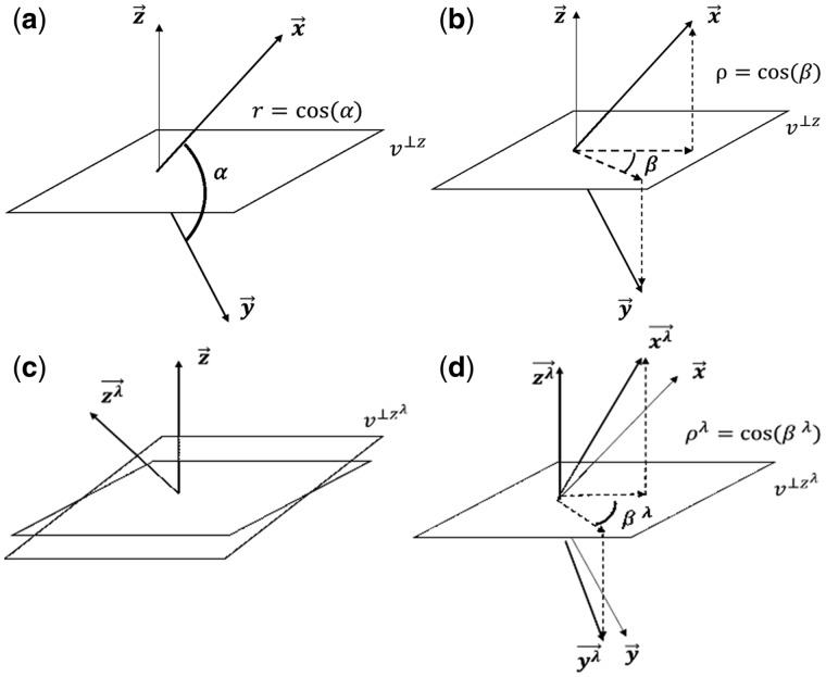
For the purpose of illustration consider three random variables $X, Y$, and $Z$ with expectation zero ($E\left[X\right]=E\left[Y\right]=E\left[Z\right]=0$). Their respective vector representations are denoted by ${\displaystyle \overrightarrow{\mathit{x}}},{\displaystyle \overrightarrow{\mathit{y}}},{\displaystyle \overrightarrow{\mathit{z}}}$. The correlation $r$ between $X$ and $Y$ (a measure of linear dependence) is related to the angle between the vectors (see Fig. 1a), and can be written as

$$r_{\mathit{XY}}=\frac{\sum _{i=1}^n\left(x_i-{\displaystyle \stackrel{-}{x}}\right)\left(y_i-{\displaystyle \stackrel{-}{y}}\right)}{\sqrt{{\sum _{i=1}^n\left(x_i-{\displaystyle \stackrel{-}{x}}\right)}^2}\sqrt{{\sum _{i=1}^n\left(y_i-{\displaystyle \stackrel{-}{y}}\right)}^2}}=\frac{{\displaystyle \overrightarrow{\mathit{x}}}·{\displaystyle \overrightarrow{\mathit{y}}}}{{\Vert {\displaystyle \overrightarrow{\mathit{x}}}\Vert }_2{\Vert {\displaystyle \overrightarrow{\mathit{y}}}\Vert }_2}$$ (5)

where ${\Vert {\displaystyle \overrightarrow{\mathit{*}}}\Vert }_2$ denotes the usual Euclidean norm, and ${\displaystyle \overrightarrow{\mathit{x}}}·{\displaystyle \overrightarrow{\mathit{y}}}={\Vert {\displaystyle \overrightarrow{\mathit{x}}}\Vert }_2{\Vert {\displaystyle \overrightarrow{\mathit{y}}}\Vert }_2\cos (\angle {\displaystyle \overrightarrow{\mathit{x}}},{\displaystyle \overrightarrow{\mathit{y}}})$and $\angle {\displaystyle \overrightarrow{\mathit{x}}},{\displaystyle \overrightarrow{\mathit{y}}}$ stands for the angle between ${\displaystyle \overrightarrow{\mathit{x}}}$ and ${\displaystyle \overrightarrow{\mathit{y}}}$. In the multivariate case, the pairwise correlations can be arranged in a symmetric matrix (i.e. the correlation matrix). This matrix is the covariance matrix of the standardized random variables, and its pairwise association are in $[-1,1]$.

Fig. 1.

Geometry of the partial correlation. The vectors ${\displaystyle \overrightarrow{\mathit{x}}}$, ${\displaystyle \overrightarrow{\mathit{y}}}$ and ${\displaystyle \overrightarrow{\mathit{z}}}$ represent the random variables X, Y and Z  in subject space. In Panel (a), the correlation $\mathit{r}$ between X and Y is the cosine of $\alpha$. In Panel (b), the partial correlation between X and Y can be interpreted as the cosine of the angle $\beta$. That is the cosine between the projection of ${\displaystyle \overrightarrow{\mathit{x}}}$ and ${\displaystyle \overrightarrow{\mathit{y}}}$ onto a plane orthogonal to ${\displaystyle \overrightarrow{\mathit{z}}}$. The shrinkage effect consists in that the vectors ${\displaystyle \overrightarrow{\mathit{x}}}$, ${\displaystyle \overrightarrow{\mathit{y}}}$ and ${\displaystyle \overrightarrow{\mathit{z}}}$are transformed to ${\displaystyle \overrightarrow{{\mathit{x}}^{\mathit{\lambda }}}}, {\displaystyle \overrightarrow{{\mathit{y}}^{\mathit{\lambda }}}}$ and ${\displaystyle \overrightarrow{{\mathit{z}}^{\mathit{\lambda }}}}$ such that their lengths remain 1, and only the angles between each other change. In other words, the transformed vectors become less correlated. In Panel (c), the geometrical effect of the shrinkage consists in changing the projection plane ${\mathit{v}}^{\perp \mathit{z}}$ to ${\mathit{v}}^{\perp {\mathit{z}}^{\mathit{\lambda }}}$. In Panel (d), the ‘shrunk’ partial correlation ${\rho }^{\lambda }$ between X and Y is the cosine of the angle ${\beta }^{\lambda }$. That is the cosine between the projections of ${\displaystyle \overrightarrow{{\mathit{x}}^{\mathit{\lambda }}}}$ and ${\displaystyle \overrightarrow{{\mathit{y}}^{\mathit{\lambda }}}}$ onto ${\mathit{v}}^{\perp {\mathit{z}}^{\mathit{\lambda }}}$

Whenever the target matrix $\mathbf{T}$ in Equation (3) is chosen as the diagonal matrix of variances, it results in scaling the off-diagonal elements of ${\widehat{\mathbf{C}}}^{\mathrm{SM}}$ by a constant factor $(1-\lambda )$, while the diagonal remains unchanged. This applies as well to the correlation matrix with a shrinkage towards the identity matrix; symbolically ${r^{\lambda }}_{\mathit{ij}}=\left(1-\lambda \right)r_{\mathit{ij}} \forall i\ne j$, and 1 otherwise. In this case, the maximal correlation is $\pm (1-\lambda )$, and (near) multi-collinearity is avoided. In subject space, this decorrelation means that the angles between the vectors increase while their lengths remain equal to one, generating the new ${\displaystyle \overrightarrow{{\mathit{x}}^{\mathit{\lambda }}}},{\displaystyle \overrightarrow{{\mathit{y}}^{\mathit{\lambda }}}},{\displaystyle \overrightarrow{{\mathit{z}}^{\mathit{\lambda }}}}$.

On the other hand, the (standard) partial correlation $\rho$ is a measure of linear dependence between two random variables after conditioning over all others. Geometrically, conditioning $X$ (and $Y$) over the variable $Z$ is equivalent to projecting the vector ${\displaystyle \overrightarrow{\mathit{x}}}$ (and ${\displaystyle \overrightarrow{\mathit{y}}}$) onto a plane $v^{\perp Z}$orthogonal to ${\displaystyle \overrightarrow{\mathit{z}}}$. Therefore, $\rho$ is the cosine of the angle between the projected vectors on $v^{\perp Z}$ as shown in Figure 1b. The new vectors (i.e. ${\displaystyle \overrightarrow{{\mathit{x}}^{\mathit{\lambda }}}},{\displaystyle \overrightarrow{{\mathit{y}}^{\mathit{\lambda }}}}$) are now projected onto a new plane (i.e. $v^{\perp z^{\lambda }}$), propagating the shrinkage effects as shown in Figure 1c and d. At this point we recognize that the same geometric arguments used in Fisher (1924) to obtain the distribution of the (standard) partial correlation hold. From here on we will adapt that reasoning to our context.

We start by highlighting that $r^{\lambda }$ =$\left(1-\lambda \right)r$ is invariant under rotations of the axes (like $r$). In other words, given a rotation of the coordinates, the shrunk (and standard) correlation remains unchanged. Now, suppose that the coordinate system rotates making one of its axes coincides with ${\displaystyle \overrightarrow{{\mathit{z}}^{\mathit{\lambda }}}}$ (the new conditioning variable). Then, conditioning over $Z^{\lambda }$ becomes equivalent to removing (from ${\displaystyle \overrightarrow{{\mathit{x}}^{\mathit{\lambda }}}}$ and ${\displaystyle \overrightarrow{{\mathit{y}}^{\mathit{\lambda }}}}$) the component in the ${\displaystyle \overrightarrow{{\mathit{z}}^{\mathit{\lambda }}}}$ direction. Thus, the vectors are projected onto a plane $v^{\perp Z^{\lambda }}$ that is orthogonal to ${\displaystyle \overrightarrow{{\mathit{z}}^{\mathit{\lambda }}}}$. Consequently, $r^{\lambda }$ is modified when it is conditioned over $Z^{\lambda }$ to give the ‘shrunk’ partial correlation ${\rho }^{\lambda }$; symbolically ${\rho }^{\lambda }=r^{\lambda }|Z^{\lambda }$. The distribution of $r^{\lambda }|Z^{\lambda }$ is the distribution of $r^{\lambda }$ obtained by removing one sample (decreasing its degrees of freedom by one). This process can be repeated by rotating the axes once more to condition over the next variable, and the argument is generalizable by replacing $Z$ with a set of $p-2$ variables $\{Z_1,Z_2,., Z_{p-2}\}$. Finally, the vectors have been conditioned over the $p-2$ other variables, and ${\rho }^{\lambda }=r^{\lambda }\left|\right\{Z_1,Z_2,., Z_{p-2}\}$ follows the distribution of $r^{\lambda }$ obtained after removing $p-2$ samples.

The distribution for $r^{\lambda }$ is found via the transformation $r^{\lambda }=(1-\lambda )r$ over Equation (4) leading to

$${\int }_{-1}^1{f}_0\left(r\right)dr={\int }_{-\left(1-\lambda \right) }^{\left(1-\lambda \right) }{f}_0\left(\frac{r^{\lambda }}{\left(1-\lambda \right) }\right)\frac{d{r}^{\lambda }}{\left(1-\lambda \right) }=1$$ (6)

and is naturally defined in $[-(1-\lambda ),(1-\lambda \left)\right]$ with the form

$${f_0}^{\lambda }\left(r^{\lambda }\right)=\frac{{\left({\left(1-\lambda \right)}^2-{\left(r^{\lambda }\right)}^2\right)}^{(k-3)/2}}{\mathit{Beta}\left(\frac{1}{2},\frac{k-1}{2}\right){\left(1-\lambda \right) }^{(k-2)}}$$ (7)

The expectation is $\mathbb{E}\left[r^{\lambda }\right]=\left(1-\lambda \right)\mathbb{E}\left[r\right]$, and its variance $\mathrm{var}\left[r^{\lambda }\right]={\left(1-\lambda \right)}^2\mathrm{v}\mathrm{ar}\left[r\right]$ is reduced as ${\left(1-\lambda \right)}^2\le 1$. As a consequence of the geometric arguments above the density for the ‘shrunk’ partial correlation${\rho }^{\lambda }=r^{\lambda }\left|\mathrm{ }\right\{Z_1,Z_2,., Z_{p-2}\}$ in the well posed case $n\gg p$ is also described by Equation (7) with $k=n-1-(p-2)$. In the ill-posed case $n<p$, $k$ can be estimated via maximum likelihood estimation (MLE) (Supplementary Section S2) as it has no clear geometrical meaning. Some examples of the shrinkage effect are provided in the Supplementary Section S1. Further mathematical details can be found in Fisher (1915) and Hotelling (1953).

3 Implementation

In what follows we will compare two inference methods. First, ENF with Equation (4) currently implemented in GeneNet version 1.2.13 (see Section 2.2). Second, the parametric approach proposed here, to which we will refer as Shrunk MLE (see Supplementary Section S2). We will employ as the gold standard a computationally expensive estimation of P-values based on Monte Carlo (MC) (see Supplementary Section S3). MC estimation is a non-parametric and unbiased method; however, for large networks it is time costly which limits its use in many applications.

3.1 Synthetic data

Simulations are performed with R version 3.4.0, and GeneNet version 1.2.13. The later allows to generate GGMs with a fixed percentage of partial correlations (Schäfer and Strimmer, 2005a).

3.2 Stress response in Escherichia coli

This dataset consists of E.coli microarray gene-expression from Schmidt-Heck et al. (2004). The authors studied the stress temporal response after the expression of recombinant human superoxide dismutase (SOD) at 8, 15, 22, 45, 68, 90, 150 and 180 min. SOD expression was induced by isopropyl β-D-1-thiogalactopyranoside (IPTG), which is a lactose analog inducer of the lac operon. In the original study the authors identified 102 out of 4289 protein coding genes as differentially expressed at transcript level in one or more samples after induction. Data pre-processing included log₂-ratio transformation with respect to the first time point. The final dataset consists of expression values for transcripts corresponding to 102 genes with 9 time points, and was obtained from the R package GeneNet version 1.2.13.

3.3 Infection response in Mus musculus

The following dataset comes from a study of transcript interactions in a mouse (M.musculus) model of influenza infection (Steed et al., 2017). It is available at https://www.ebi.ac.uk/arrayexpress/experiments/E-MTAB-5337, and consists of RNA-seq transcript expression data of mouse lungs. The study focuses on the role of the Irgm1 gene in mice of 8–12 weeks of age with samples at four time points (0, 3, 6, and 10 days after infection). We pre-processed it by filtering out probes with low counts (i.e. fractions per million (FPM) < 1). From the duplicate probes we kept the one with the highest FPM. A total of 539 genes were differentially expressed at the 10% level false discovery rate (FDR) and their expression values were log₂-transformed.

4 Results

4.1 Analysis of simulated data

In this section, we demonstrate the superior performance of the improved approach Shrunk MLE by comparing it to: (i) ENF, and (ii) MC P-value estimation. A total of 4574 datasets were simulated (see Supplementary Table S1). First, we perform a qualitative study under the null hypothesis $H_0:\rho =0$. Second, we cross compare the reconstruction for sparse networks (i.e. small percentage of true positives) in terms of the FPs, and the positive predictive value (PPV). Third, two real quantitative molecular profile datasets are used to examine the results from a biological point of view. Supplementary Table S2 gives an overview of definitions used in the evaluation.

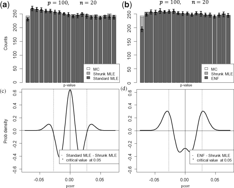
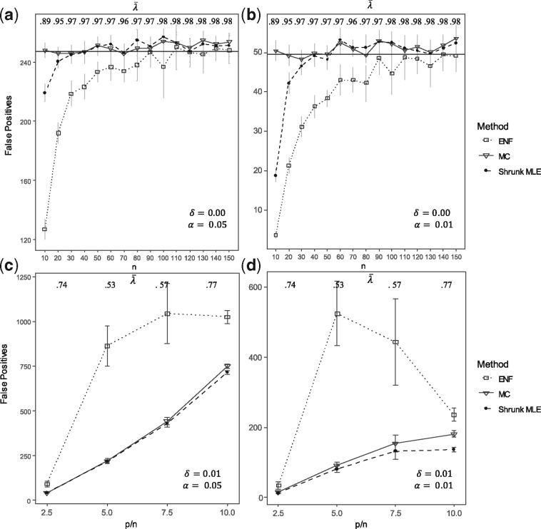
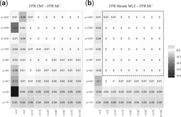
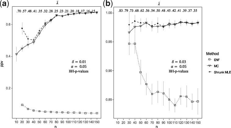
Figure 2a and b display the average histograms for the P-values retrieved by each method. Figure 2c and d show the two null-densities$\mathrm{ }{f}_0\left({\rho }^{\lambda }\right)$ and ${f_0}^{\lambda }\left({\rho }^{\lambda }\right)\mathrm{ }$presented as Equations (4) and (7). In the first case, the degrees of freedom $k$ was obtained via MLE under simulated $H_0$, in the second case via ENF. Here it can be observed that $f_0\left({\rho }^{\lambda }\right)$ has larger tails than ${f_0}^{\lambda }\left({\rho }^{\lambda }\right)$. This is further illustrated by Q-Q plots in Supplementary Figure S2, where the P-values’ quantiles are expected to be on the diagonal line if they agree with the theoretical quantiles (from a uniform distribution in $[0,1]$). Figure 3 shows the number of significant partial correlations obtained by each method while varying the sample size $n$. Figure 3a and b show the results using (un-adjusted) P-values under $H_0$ at $\alpha =0.05$ and $\alpha =0.01$ respectively. It can be observed that ENF does not recover the proportion of expected FPs. Figure 3c and d show the FPs for different ratios $p/n$ in sparse networks. In this scenario, ENF learns considerably more FPs than the other methods. In Figure 4, we compare the false positive rate (FPR) with respect to the gold standard in a grid of $p$ and $n$. For Shrunk MLE the performance is equivalent to MC when $n>10$ and $p>40$, while ENF differs in almost every case. The PPV for different $n$ is presented in Figure 5 for adjusted P-values (Benjamini and Hochberg, 1995). See Supplementary Figures S3 and S4 for the PPV with unadjusted P-values, and an additional Type I error plot. In general, a relatively low PPV is expected as $\delta$ is small (i.e. there are few positives compared with the number of tests). We observe that the performance of Shrunk MLE is similar to the gold standard MC even for very large $\lambda$. Additionally, Shrunk MLE requires a much shorter computational time, as can be seen in the Supplementary Table S3.

Fig. 2.

Probability densities and P-values under$\mathrm{ }{H}_0$. This figure shows a comparison of the standard $f_0\left({\rho }^{\lambda }\right)$ and ‘shrunk’ ${f_0}^{\lambda }\left({\rho }^{\lambda }\right)$ densities, and their P-values under $H_0$. Here Standard MLE denotes $f_0\left({\rho }^{\lambda }\right)$ (i.e. Equation 4) with k obtained via MLE (as in Shrunk MLE). Panel (a) shows the average histogram of P-values obtained with (i) Standard MLE (dark grey), (ii) Shrunk MLE (light grey) and (iii) MC (white) with 15 iterations. Panel (b) replaces Standard MLE by ENF to estimate $k$ in $f_0\left({\rho }^{\lambda }\right)$ (currently used in GeneNet). The bin’s width is set to 0.05; therefore, the first bin represents the amount of significant coefficients at the 5% level. The bin’s height corresponds to the mean over 25 simulations, and the error bars (for ENF) to ±2 SE. It can be seen that the P-values from ENF (dark grey) are not uniformly distributed in [0, 1] under $H_0$. Panels (c) and (d) show the difference $f_0\left({\rho }^{\lambda }\right)-{f_0}^{\lambda }\left({\rho }^{\lambda }\right)$ when $k$ is found via MLE or via ENF, respectively (see Section 2.1). Data were simulated with $p=100$, $n=20$ and $\lambda =$0.94. The critical value at $\alpha =0.05$ (in dashed grey) is estimated by MC (with 100 iterations). It can be seen that $f_0\left({\rho }^{\lambda }\right)$ has larger tails than ${f_0}^{\lambda }\left({\rho }^{\lambda }\right)$

Fig. 3.

False positives. This figure shows the number of FPs obtained with different sample size $n$. The number of FPs are shown in Panels (a) and (b) under $H_0$: no partial correlation (i.e. the percentages of true correlations $\delta$ is zero). Inference is carried out from simulated data for $p$ = 100 and $n$ ranging from 10 to 150 in steps of size 10. The black horizontal line represents the expected number of FPs under$\mathrm{ }{H}_0$, tested at $\alpha$ = 0.05 and$\mathrm{ }0.01$ respectively (i.e. 247.5 for $\alpha$ = 0.05 and 49.5 for $\alpha$=0.01). Panels (c) and (d) show the number of FPs for different proportions $p/n$ when the percentages of non-zero correlations is $\delta$ = 0.01. Here $p$ = 50, 100, 150, 200 and $n$ = 20. Three approaches are compared: ENF (dot with dashed line), Shrunk MLE (square with dotted line), and MC with 15 iterations (triangle with continuous line). Symbols (and bars) represent the average (±2 SE) over 25 repeated simulations. The upper horizontal axis shows the average shrinkage intensity $\stackrel{}{\mathrm{\lambda }}$ rounded to two digits

Fig. 4.

FPR cross-comparison. This figure shows a heatmap for the difference in FPR under $H_0$: no partial correlation with respect to the gold standard (MC). The number of variables $p$ range from 10 to 400, and the sample size $n$ from 3 to 100. Panel (a) shows the heatmap for the FPR for ENF minus the FPR for MC, averaged over 10 simulations (rounded to two decimals). Panel (b) show the respective results for Shrunk MLE. The test is carried out at $\alpha$ = 0.05 with a shrinkage value fixed to $\lambda$ = 0.3. The color scale represents the FPR differences in the $p$ – $n$ grid, where the larger the FPR difference the darker is the corresponding grid cell. In general, Shrunk MLE outperforms ENF, and it is in close agreement with MC for $p>40$ and $n>10$

Fig. 5.

Positive predictive value. This figure shows the PPV ($\mathit{PPV}=\mathit{TP}/\mathit{P}$) obtained with different sample sizes. The inference is carried out from simulated data for $p$ =100 with $n$ ranging from 10 to 150 in steps of size 10, tested at $\alpha$ = 0.05. The Panels (a) and (b) show the PPV using Benjamini-Hochberg (BH)-adjusted P-values for multiple testing with $\delta$ = 0.01 (or 49 correlations) and $\delta$ = 0.03 (or 148 correlations). Three approaches are compared: ENF (dot with dashed line), Shrunk MLE (square with dotted line), and MC with 15 iterations (triangle with continuous line). Symbols (and bars) represent the average (±2 SEs) over 25 repeated simulations. The upper horizontal axis shows the average shrinkage intensity $\overline{\mathrm{\lambda }}$ rounded to two digits

4.2 Analysis of experimental data

4.2.1 Effects of human SOD protein expression on transcript expression in E.coli

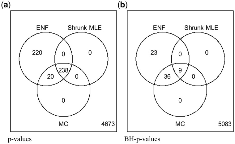
Here we employ our new approach to analyze E.coli microarray gene-expression data from Schmidt-Heck et al. (2004). The final data consist of transcripts corresponding to 102 genes with 9 time points. We treated the data as static (ignoring its temporal nature) following the original analysis (Schäfer and Strimmer, 2005a). Figure 6 shows that MC, and our approach (Shrunk MLE) learn nearly the same amount of edges using P-values, differing in 20 out of 258 connections (∼7.75%).

Fig. 6.

Amount of significant edges related to the induced expression of SOD in E.coli. Analysis of E.coli gene microarray expression data upon response to induced SOD expression. The dataset includes 102 genes (Schmidt-Heck et al., 2004). The estimator produces an optimal shrinkage $\lambda$ = 0.18. Three methods are compared at $\alpha$ = 0.05: ENF, Shrunk MLE, MC with 40 iterations. Panel (a) Venn diagram of significant partial correlations (i.e. edges in the GGM) recovered by each method with un-adjusted P-values. Panel (b) Venn diagram of significant partial correlations recovered by each method with BH-adjusted P-values

ENF learns 220 additional edges (∼85.3% more than MC). We observe that after BH adjustment the amount of edges in Shrunk MLE is too low to make any conclusion due to the small sample size (see Figs 3–5). Therefore, the analysis is continued with un-adjusted P-values. For every method the most significant connections were lacA-lacZ, lacY-lacZ and lacA-lacY. The lac operon involves precisely these three genes induced by IPTG. Shrunk MLE and MC retrieve 74 connected genes, and ENF 88 at $\alpha =0.05$. These genes were assessed for gene ontology (GO) enrichment using PANTHER Classification System (http://geneontology.org/) (Ashburner et al., 2000; Mi et al., 2017) with a FDR < 0.05. The result shows that our method identifies a significant enrichment of stress response (GO: 0006950, fold enrichment = 2.57, FDR = 3.87 10⁻²). In contrast, this GO term is not significant for ENF (fold enrichment = 9.81, FDR = 1.27 10⁻¹) suggesting that the enrichment of the genes related to the treatment stimulus was diluted. The most significant GOs obtained with Shrunk MLE, ENF, as well as the hubs present in the network structures are reported in Supplementary Table S4a–c, respectively. The GGM structure can be seen in Supplementary Figure S5.

4.2.2 Effects of infection with the influenza virus on gene expression in M.musculus

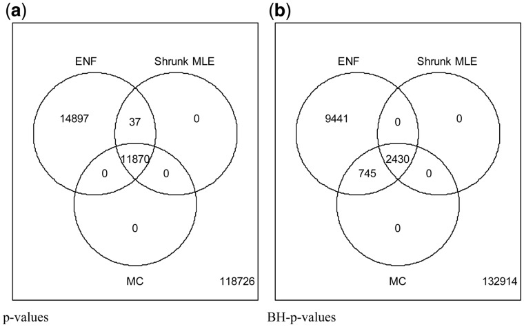
Here we study transcript interactions in a public RNA-seq data from a mouse (M.musculus) model of influenza infection (Steed et al., 2017). The final data consists of 539 genes and 2$4$ samples. Figure 7 shows that MC (considered as the gold standard), and Shrunk MLE learn nearly the same number of edges using P-values, differing only in 37 out of 11 870 connections (∼0.312%). It also shows that the agreement using BH-adjusted P-values is ∼76.53%. This illustrates the fact that even small discrepancies in the P-values might become large for the adjusted P-values, and can be observed by comparing the PPVs in Figure 5 and Supplementary Figure S3.

Fig. 7.

Amount of significant edges related to lung samples’ expression in M.musculus. Analysis of M.musculus RNA-seq expression data from lung samples (Steed et al., 2017). The estimator produces an optimal shrinkage $\lambda \approx$0.11. Three methods are compared at $\alpha =0.10$; ENF, Shrunk MLE and MC (with 40 iterations). Panel (a) Venn diagram of significant partial correlations (i.e. edges in the GGM) recovered by each method with un-adjusted P-values. Panel (b) Venn diagram of significant partial correlations recovered by each method with BH-adjusted P-values

ENF learns considerably more edges (∼200%) compared with MC or to our method. As the large number of genes is uninformative for GO enrichment analysis the edges were assessed in terms of true positive rate (TPR) and FPR by using as ground truth the protein-protein interaction STRING database (https://string-db.org/) (Szklarczyk et al., 2017) (see Supplementary Table S5a). We observe that while the TPR for Shrunk MLE and ENF are similar, the FPR is lower for Shrunk MLE. Moreover, not a single additional connection found exclusively by ENF is reported in the STRING database. The most significant GOs found with Shrunk MLE, and ENF are reported in Supplementary Table S5b and c, and the GGM structure in Supplementary Figure S6.

5 Discussion

GGMs assess linear relationships between pairs of variables (partial correlations) from multivariate normal data. Some pitfalls inherent to the model are that non-linear associations are not necessarily captured, and that the partial correlation is not a robust statistics (i.e. it is susceptible to outliers), which becomes important when the sample size is small. The motivation for this work has been to improve the inference of GGMs from quantitative molecular profile data when sample size is small (e.g. 10–20), and there is large number of variables (100–10 000). Inferring a GGM structure demands the inverse of the covariance matrix, which is ill-conditioned in the high-dimensional scenario. Covariance estimators based on shrinkage are broadly employed in these cases, resulting in an invertible matrix. Previously, a parametric tests for GGMs was designed that calibrates the P-values in a approximated way, using the standard density and ENF. The inference becomes suboptimal because the shrinkage effects are not included in the test density. Moreover, ENF is known to be susceptible to errors as the selection of a non-contaminated region is difficult (i.e. it is restricted to sparse networks). An accurate ‘shrunk’ test is needed to complement the estimation with a proper control of the Type I error (i.e. FPR), and multiple testing corrections. In this way, experiments performed with different sample sizes and/or number of compounds (nodes) become comparable.

Our empirical results support the idea that the standard density has larger tails than the new ‘shrunk’ density. As a consequence (i) under$\mathrm{ }{H}_0\mathrm{ }$the P-values deviate from $U[0,1]$, and (ii) the FPs cannot be controlled efficiently by multiple testing procedures. When it comes to its biological interpretation the excessive number of FPs might dilute the GO enrichment related to the treatment stimulus (see E.coli example) thus obscuring the targeted effect of the analysis.

To resolve this situation, we have derived the null distribution of the ‘shrunk’ (i.e. regularized) partial correlation. In this sense, our work represents an improvement over the parametric tests described in Schäfer and Strimmer (2005a,b). To our knowledge, this is the only approach with a theoretical test of significance that includes the shrinkage effect. This was achieved by recalling some the geometrical ideas about the partial correlation coefficient from the seminal work of Fisher (1924). The improved approach presented here (i.e. Shrunk MLE) is independent of the aforementioned drawbacks because it naturally includes the shrinkage, and the degrees of freedom are estimated independently of the real mixture. We have shown how the test with Shrunk MLE (i) allows the inference for any shrinkage value with accurate multiple testing corrections (e.g. control of the FDR), (ii) it is as accurate as MC P-value estimation (a non-parametric approach considered to be the gold standard) while computationally faster and (iii) it is not limited to sparse networks. The assessment was carried out in terms of the number of learnt edges, and the PPV (with and without adjustment). Particularly, for $p>40$ and $n>10$ the FPR is as accurate as MC (see Fig. 4). However, for dataset with too small sample size (e.g. $n$ = 5 and $p$ = 20 in Fig. 4) the estimation should be performed with MC.

Ideally, an analysis should include both the coefficient and its P-value. However, without considering $\lambda$, it is not trivial to conclude by the ‘shrunk’ coefficient whether an association is strong or not. Further studies are required to address this issue.

Funding

This work was supported by the Data Science and System Complexity Centre (DSSC) of the University of Groningen. M.G. is supported by the European Cooperation in Science and Technology (COST) [COST Action CA15109 European Cooperation for Statistics of Network Data Science (COSTNET)].

Conflict of Interest: none declared.

References

- Ashburner M. et al. (2000) Gene ontology: tool for the unification of biology. Nat. Genet., 25, 25.. [DOI] [PMC free article] [PubMed] [Google Scholar]
- Beerenwinkel N. et al. (2007) Genetic progression and the waiting time to cancer. PLoS Comput. Biol., 3, e225.. [DOI] [PMC free article] [PubMed] [Google Scholar]
- Benedetti E. et al. (2017) Network inference from glycoproteomics data reveals new reactions in the IgG glycosylation pathway. Nat. Commun., 8, 1483. [DOI] [PMC free article] [PubMed] [Google Scholar]
- Benjamini Y., Yosef H. (1995) Controlling the false discovery rate: a practical and powerful approach to multiple testing. J R Stat Soc Series B Stat Methodol., 57, 289–300. [Google Scholar]
- Butte A.J., Kohane I.S. (2003) Relevance networks: a first step toward finding genetic regulatory networks within microarray data In: Parmigiani G.et al. (ed.) The Analysis of Gene Expression Data. Springer, New York, NY, pp. 428–446. [Google Scholar]
- Edwards D. (2000) Introduction to Graphical Modelling, 2nd edn. Springer Science & Business Media, Springer-Verlag; New York. [Google Scholar]
- Efron B. (2012) Large-Scale Inference: Empirical Bayes Methods for Estimation, Testing, and Prediction. Cambridge University Press, New York. [Google Scholar]
- Efron B. (2004) Large-scale simultaneous hypothesis testing: the choice of a null hypothesis. J. Am. Stat. Assoc., 99, 96–104. [Google Scholar]
- Efron B. (2005) Local false discovery rates. Stanford University.
- Faust K., Raes J. (2012) Microbial interactions: from networks to models. Nat. Rev. Microbiol., 10, 538.. [DOI] [PubMed] [Google Scholar]
- Fisher R.A. (1915) Frequency distribution of the values of the correlation coefficient in samples from an indefinitely large population. Biometrika, 10, 507–521. [Google Scholar]
- Fisher R.A. (1924) The distribution of the partial correlation coefficient. Metron, 3, 329–332. [Google Scholar]
- Friedman J. et al. (2008) Sparse inverse covariance estimation with the graphical lasso. Biostatistics, 9, 432–441. [DOI] [PMC free article] [PubMed] [Google Scholar]
- Friedman N. et al. (2000) Using Bayesian networks to analyze expression data. J. Comput. Biol., 7, 601–620. [DOI] [PubMed] [Google Scholar]
- Hotelling H. (1953) New light on the correlation coefficient and its transforms. J. R. Stat. Soc. Ser. B, 15, 193–232. [Google Scholar]
- Keller M.P. et al. (2008) A gene expression network model of type 2 diabetes links cell cycle regulation in islets with diabetes susceptibility. Genome Res., 18, 706–716. [DOI] [PMC free article] [PubMed] [Google Scholar]
- Ledoit O., Wolf M. (2004) A well-conditioned estimator for large-dimensional covariance matrices. J. Multivar. Anal., 88, 365–411. [Google Scholar]
- Ledoit O., Wolf M. (2003) Improved estimation of the covariance matrix of stock returns with an application to portfolio selection. J. Empir. Financ., 10, 603–621. [Google Scholar]
- Lemm S. et al. (2011) Introduction to machine learning for brain imaging. Neuroimage, 56, 387–399. [DOI] [PubMed] [Google Scholar]
- Ma S. et al. (2007) An Arabidopsis gene network based on the graphical Gaussian model. Genome Res., 17, 1614–1625. [DOI] [PMC free article] [PubMed] [Google Scholar]
- Markowetz F., Spang R. (2007) Inferring cellular networks - a review. BMC Bioinformatics, 8, S5. [DOI] [PMC free article] [PubMed] [Google Scholar]
- Mi H. et al. (2017) PANTHER version 11: expanded annotation data from Gene Ontology and Reactome pathways, and data analysis tool enhancements. Nucleic Acids Res., 45, D183–D189. [DOI] [PMC free article] [PubMed] [Google Scholar]
- Omranian N. et al. (2016) Gene regulatory network inference using fused LASSO on multiple data sets. Sci. Rep., 6, 20533.. [DOI] [PMC free article] [PubMed] [Google Scholar]
- Saha A. et al. (2017) Co-expression networks reveal the tissue-specific regulation of transcription and splicing. Genome Res., 11, 1843–1858. [DOI] [PMC free article] [PubMed] [Google Scholar]
- Schäfer J., Strimmer K. (2005a) A shrinkage approach to large-scale covariance matrix estimation and implications for functional genomics. Stat. Appl. Genet. Mol. Biol., 4, 1175–1189. [DOI] [PubMed] [Google Scholar]
- Schäfer J., Strimmer K. (2005b) An empirical Bayes approach to inferring large-scale gene association networks. Bioinformatics, 21, 754–764. [DOI] [PubMed] [Google Scholar]
- Schmidt-Heck W. et al. (2004) Reverse engineering of the stress response during expression of a recombinant protein. In: Proceedings of the EUNITE Symposium, 10–12 June 2004, Aachen, Germany pp. 407–412. Verlag Mainz. [Google Scholar]
- Steed A.L. et al. (2017) The microbial metabolite desaminotyrosine protects from influenza through type I interferon. Science, 357, 498–502. [DOI] [PMC free article] [PubMed] [Google Scholar]
- Strimmer K. (2008a) A unified approach to false discovery rate estimation. BMC Bioinformatics, 9, 303.. [DOI] [PMC free article] [PubMed] [Google Scholar]
- Strimmer K. (2008b) fdrtool: a versatile R package for estimating local and tail area-based false discovery rates. Bioinformatics, 24, 1461–1462. [DOI] [PubMed] [Google Scholar]
- Szklarczyk D. et al. (2017) The STRING database in 2017: quality-controlled protein-protein association networks, made broadly accessible. Nucleic Acids Res., 45, D362–D368. [DOI] [PMC free article] [PubMed] [Google Scholar]
- Werhli A.V. et al. (2006) Comparative evaluation of reverse engineering gene regulatory networks with relevance networks, graphical Gaussian models and Bayesian networks. Bioinformatics, 22, 2523–2531. [DOI] [PubMed] [Google Scholar]
- Whittaker J. (1990) Graphical Models in Applied Multivariate Statistics. Wiley Publishing, NY. [Google Scholar]
- Wickens T.D. (2014) The Geometry of Multivariate Statistics. Psychology Press, New York. [Google Scholar]
Associated Data
This section collects any data citations, data availability statements, or supplementary materials included in this article.