Abstract
mrgsolve is an open‐source R package available on the Comprehensive R Archive Network. It combines R and C++ coding for simulation from hierarchical, ordinary differential equation–based models. Its efficient simulation engine and integration into a parallelizable, R‐based workflow makes mrgsolve a convenient tool both for simple and complex models and thus is ideal for physiologically‐based pharmacokinetic (PBPK) and quantitative systems pharmacology (QSP) model. This tutorial will first introduce the basics of the mrgsolve simulation workflow, including model specification, the introduction of interventions (dosing events) into the simulation, and simulated results postprocessing. An applied simulation example is then presented using a PBPK model for voriconazole, including a model validation step against adult and pediatric data sets. A final simulation example is then presented using a previously published QSP model for mitogen‐activated protein kinase signaling in colorectal cancer, illustrating population simulation of different combination therapies.
mrgsolve Structure
mrgsolve is distributed as an R package that is freely available on the Comprehensive R Archive Network (CRAN; https://cran.r-project.org/web/packages/mrgsolve/index.html). The mrgsolve package uses Livermore Solver for Ordinary Differential Equations, an ordinary differential equation (ODE) solver from the ODEPACK1 library, which is interfaced with R through the Rcpp2 package. C++ classes were developed to abstract solver setup, data sets and records, and pharmacokinetic (PK) dosing events. S4 classes and methods were created to represent the model in R as an updatable object. The modeler creates a model specification file consisting of R and C++ code that is parsed, compiled, and dynamically loaded into the R session. Input data are passed in, and simulated data are returned as R objects, so disk access is never required during the simulation cycle after compiling. The resulting computational efficiency facilitates model exploration and application both during model development and decision‐making phases of a drug development program. mrgsolve features include the following:
NM‐TRAN‐like input data sets3
Bolus, infusion, compartment on/off, and reset functionality
Bioavailability, absorption lag, steady‐state, interdose interval, additional doses, model event times
Multivariate normal random effects simulated using RcppArmadillo4
Compatible with parameter estimation and design packages in R (nlme,5 saemix,6 PopED,7 PFIM8)
Integration with data summary (dplyr9) and plotting (ggplot,9 lattice10) packages
Parallelization with existing R infrastructure (mclapply11) or Sun Grid Engine (qapply12)
Compatible with output from many different model estimation platforms
Easily integrated with Shiny13 to create interactive model‐visualization applications
In addition to its release on CRAN, active development of mrgsolve is documented on GitHub https://github.com/metrumresearchgroup/mrgsolve, with input and contributions encouraged and welcomed from the pharmacometrics modeling and simulation community.
Modeling and Simulation Workflow
The general modeling and simulation workflow includes an integration of mrgsolve with other packages available in R to script, in a traceable and reproducible manner, customized data handling, model development and simulation, summarization, and visualization (Figure 1 ). The model code and script to fully implement and reproduce a simple example is available in the associated GitHub repository https://github.com/metrumresearchgroup/cptpsp-tutorial-2019. The two main pieces of the mrgsolve component of this workflow, model specification and simulation, are discussed in more detail in the next sections.
Figure 1.
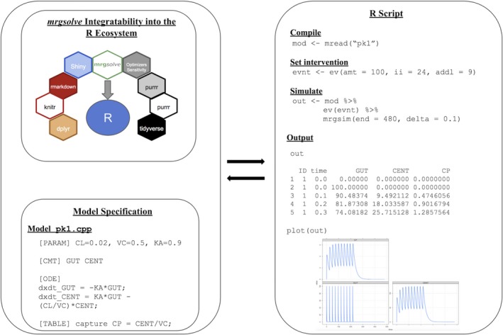
mrgsolve modeling and simulation workflow.
Model specification
The mrgsolve model specification file contains a description of the model components in different blocks. It takes a mixture of C++ and R syntax. The primary components include blocks for: model parameters ([PARAM]), state variables ([INIT], [CMT]), the ODEs ([ODE]), and outputs ([TABLE], [CAPTURE]). Each of these blocks is described in more detail and summarized (Table 1 ) in the next sections.
Table 1.
mrgsolve code blocks description
| Code block | Syntax | Comments |
|---|---|---|
| [PROB] | Text | Used to make notes about the model with no restrictions on the text entered. |
| [PARAM] | R | Used to define the parameter list in the model. |
| [CMT] | Text | Used to declare the names of all compartments in the model. Initial values are assumed to be 0. |
| [INIT] | Text | Used to declare the names and initial values of all compartments in the model. |
| [ODE] | C++ | Used to define model differential equations. |
| [TABLE] | C++ | Used to interact with parameter, compartment values, and other user‐defined variables after the system advances to the next time. |
| [MAIN] | C++ |
This code block has two main purposes:
For users who are familiar with NONMEM, [MAIN] is similar to $PK. The MAIN function gets called just prior to advancing the system from the current time to the next time for each record in the data set. [MAIN] also gets called several times before starting the problem and just prior to simulating each individual in the population. Finally, it gets called every time the model initial conditions are queried with init(). |
| [GLOBAL] | C++ |
This block is for writing C++ code that is outside of [MAIN], [ODE] and [TABLE]. There is no artificial limit on what sort of C++ code can go in [GLOBAL]; however, there are two more common uses:
|
| [PREAMBLE] | C++ |
This block is called once in two different settings:
[PREAMBLE] is a function that allows you to set up your C++ environment. It is only called one time during the simulation run (right at the start). The code in this block is typically used to configure or initialize C++ variables or data structures that were declared in [GLOBAL]. |
| [OMEGA] | Text | Used to enter variance/covariance matrices for subject‐level random effects drawn from multivariate normal distribution. All random effects are assumed to have a mean of 0. |
| [SIGMA] | Text | Use this block to enter variance/covariance matrices for within‐subject random effects drawn from multivariate normal distribution. All random effects are assumed to have a mean of 0. |
Parameters
The parameter block [PARAM] is used to list an updatable set of name–value pairs. Although the name “parameter” may have a certain connotation in the modeling world, in mrgsolve a “parameter” could be any category of numeric data: covariates (e.g., WT, AGE, SEX), flags, and other numeric data that we commonly call “parameter” (e.g., CL or VC).
Although there may be multiple [PARAM]blocks in a model, once compiled they become condensed to a single parameter list stored in the model object. The names and values of all parameters must be declared for the model to be compiled. For example:
[PARAM] CL = 1, VC = 20, KA = 1.2
KM = 25, VMAX = 400, FLAG = 1, WT = 80
SEX = 0, N = sqrt(25)
Notably, although a default value for each parameter must be declared for compilation at model compile time, the value of any parameter may be updated without recompiling the model using either the param()function during simulation execution or through an input data set.
State variables
Similar to the parameter list, the model state variables or compartments list is a series of name–value pairs that define the number, names, and initial conditions of each state variable (compartment) in the model. Compartments are declared in one of two code blocks: [INIT] or [CMT]. Nominal initial values must be supplied for each compartment. The main difference between [INIT] and [CMT] is that [CMT] assumes a default initial value of 0 for each compartment; thus only compartment names are entered. When using [INIT], both names and values must be explicitly stated for each compartment. The initial values for each compartment can be queried with the init() function. For example:
[CMT] GUT CENT RESP
or
[INIT] GUT = 0, CENT = 0, RESP = 25
ODEs
The [ODE] block is where the ordinary differential equations are defined. For each compartment, the value of the differential equation needs to be assigned to dxdt_CMT, where CMT is the name of the compartment. The dxdt_ equation may be a function of model parameters (via [PARAM]), the current value of any compartment (CMT), or any user‐derived variable. For example:
[CMT] GUT CENT
[ODE]
dxdt_GUT = -KA*GUT;
dxdt_CENT = KA*GUT - KE*CENT;
Because the [ODE] block is written in C++, a semicolon is required at the end of each statement.
It is important to make sure that there is a dxdt_ expression defined for every compartment listed in [CMT] or [INIT], even if it is dxdt_CMT = 0. The [ODE] function is called repeatedly (at each solver step) during a simulation run. For computational efficiency it is recommended that any calculations that do not rely on recalculation at each step be included outside of [ODE], e.g., in the [MAIN] block where derived quantities also can be calculated (Table 1 ). Notably, any calculation that depends on an amount in a compartment and determines the dxdt_ expression in a model must be written in [ODE]. For example:
[CMT] CENT RESP
[PARAM] VC = 100, KE = 0.2, KOUT = 2, KIN = 100
[ODE]
double CP = CENT/VC;
double INH = CP/(IMAX+CP);
dxdt_CENT = -KE*CENT;
dxdt_RESP = KIN*(1 - INH) - RESP*KOUT;
Note that in the [ODE] block new C++ variables must be declared as double with the semicolon at the end of each line.
Outputs
When a simulation is run in mrgsolve, the time progression of the state variables (compartments) at each specified time point is returned by default. Any other variable of interest can be returned using the [CAPTURE] block that will add additional columns to the default output capturing these variables. Often users need to interact with parameters, compartment values, and other user‐defined variables after the system advances to the next time to generate new variables. The block [TABLE] can be used for this purpose and the newly generated variables can be subsequently captured in [CAPTURE]. Example:
[TABLE] double CP = CENT/VC;
[CAPTURE] CP
The [TABLE] block also uses C++ syntax, so new variables must be declared (double) and statements must end with semicolons. For convenience, the user can simply use the capture type declaration in [TABLE], and this variable would automatically be integrated in the output without the need for a [CAPTURE] block. Example:
[TABLE] capture CP = CENT/VC;
Following is a complete example of a model specification file code for a one‐compartment PK model with oral absorption:
[PARAM] CL=0.02, VC=0.5, KA=0.9
[CMT] GUT CENT
[ODE]
dxdt_GUT = -KA*GUT;
dxdt_CENT = KA*GUT - (CL/VC)*CENT;
[TABLE] capture CP = CENT/VC;
This complete model example is saved as model/pk1.cpp in the associated GitHub repository https://github.com/metrumresearchgroup/cptpsp-tutorial-2019. Additional references include a summary of the model blocks (Table 1 ) and the mrgsolve user guide: https://mrgsolve.github.io/user_guide/index.html.
Creating a model object
Prior to simulation, a model object is created to contain the mrgsolve model using the mread()function. This function will read, parse, compile, and load the model to create a model object to be used for running simulations. As an example, the following code snippet will read in the one‐compartment model pk1 saved in the relative path ../model:
library(mrgsolve)
mod <- mread("pk1", "../model")
To get information about the model, type mod in the R console:
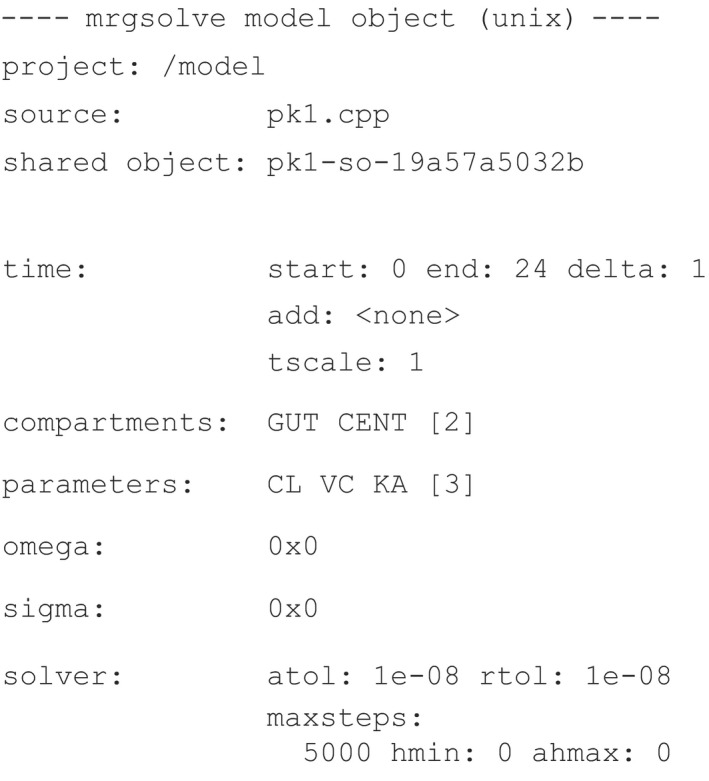
To review the model parameter values, the user can use the param() function as:
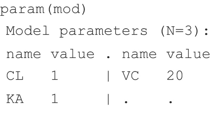
Note that the param() function can be used to explore model parameter values as above or to update those values with new values as mentioned previously. For example, if the user wants to update the CL value, the command to be used is: param(mod, CL = 2).
Setting an intervention
Setting an intervention, similar to a dosing event, can be done by creating an event object using the ev() function:
evnt <- ev(amt = 100, ii = 24, addl = 9)
This command creates the evnt object that defines a dose (amt) of 100 to be taken every day (ii; interdose interval) for 10 days (addl; nine additional doses). Intentional similarities between mrgsolve and NONMEM (ICON Development Solutions, Gaithersburg, MD) annotations were purposeful and allow, for example, the use of NM‐TRAN formatted data as input into the simulations. By default, the dose will go into compartment 1, which is the first compartment to be declared in the [INIT] or [CMT] blocks. In this example, that is the gut compartment GUT. To specify a different compartment, the user can use the ev() function cmt argument with the specific compartment number or name.
Simulating
The created model and event objects are passed to the mrgsim()function to run the simulation. The code below takes advantage of the magrittr 14 syntax %>% (available as part of the tidyverse suite9; installation and loading of the required packages is also documented and scripted through code; see mrgsolveIntro_script.R in the GitHub repository) to pass the model mod and the event evnt objects into the mrgsim() function for simulation:
out <‐ mod %>% ev(evnt) %>% mrgsim(end = 480, delta = 0.1)
The simulation output (a data frame of simulated values) is saved to the object out. Two elements of the simulation time grid—end and delta—are illustrated in the example code. These define the output end time and the interval between output time points, respectively. Other elements are start that defines the start time and add that defines any arbitrary vector of additional times to simulate. For an example of the simulation output, head(out)returns:
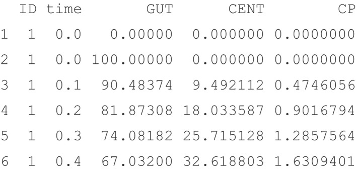
Note that the output captures the values for the two model compartments GUT and CENT as well as the captured plasma concentration CP. The same out object can be used to plot simulation results (Figure 1 ) with the function plot(out).
Additional details and examples are available on the mrgsolve GitHub page (https://github.com/metrumresearchgroup/mrgsolve) and vignettes (https://mrgsolve.github.io/vignettes/).
PBPK Application: Voriconazole
Advancements in computation capabilities have contributed to an increased use of PBPK models in recent years. These are typically mamillary models, with individual compartments representing different tissues and organs in the body. The PK of the drug of interest is described via a series of ODEs with the rates controlled by physiological properties of the species (e.g., organ volumes and blood flows) and the physicochemical properties of the drug (e.g., lipophilicity, unbound fraction, and pKa). Being based on first principles makes PBPK models particularly useful in running simulations when there are little or no clinical data available as in the case of special populations such as neonates, children, and pregnant women.
Implementation of a previously developed voriconazole PBPK model15 in mrgsolve is used as a demonstration. The PBPK model was developed by Zane and Thakker15 with the intent of providing a mechanistic explanation for the difference in voriconazole PK between adults and children. The PBPK model structure (Figure 2 ) included assumptions that the compartments were well stirred and that the transfer of drug between these compartments was flow limited. The generic flow‐limited ODEs were adapted from the previously described mass balance differential equations16, 17, 18 as follows:
| (1) |
| (2) |
| (3) |
| (4) |
| (5) |
Figure 2.
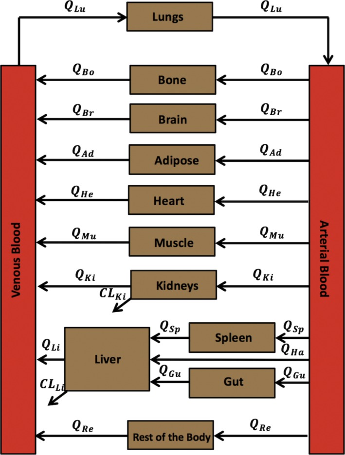
Voriconazole physiologically‐based pharmacokinetic (PBPK) model structure. The full PBPK model structure where Q represents the blood flows, CL represents clearance, and the subscripts Ad, Bo, Br, Gu, He, Ki, Li, Lu, Mu, Sp, and Re refer to adipose, bone, brain, gut, heart, kidneys, liver, lungs, muscle, spleen, and rest of the body compartments, respectively. Ha, hepatic artery.
Eqs. (1), (2), (3), (4), (5) represent the generic ODEs for noneliminating, eliminating, arterial, venous, and lung compartments, respectively, where A T is the amount of drug in tissue T; Q T is the blood flow to that tissue; C A and C V are the drug concentrations in the arterial and venous blood compartments, respectively; Kp T is the tissue:plasma partition coefficient; BP is the blood:plasma concentration ratio; CLT is the tissue clearance; and f u is the unbound fraction of drug. The specific organ subscript notations follow the same notations in Figure 2 .
The parameters required to populate the aforementioned equations were collected as follows: (i) physiological parameters including organ volumes (needed to calculate drug concentrations) and organ blood flows for the typical 30‐year‐old adult male and 5‐year‐old male child were collected from the International Commission on Radiological Protection Publication 89,19 (ii) K p values for each tissue were computed using the Poulin and Theil calculation method with inputs of drug physicochemical properties (logP, pKa, f u, and BP15, 20) and the different tissue fractional composition (water, neutral, and phospholipids) to calculate Kp values as follows20:
| (6) |
| (7) |
where Eqs. 6 and 7 were used to calculate Kp values for nonadipose and adipose tissues, respectively. P o:w is the n‐octanol:buffer partition coefficient of the nonionized species and is the olive oil:buffer partition coefficient of both the nonionized and ionized species at pH 7.4. f nl, f ph and f w are the fractional volumes of neutral lipids, phospholipids, and water, respectively. f u is the unbound fraction of drug. The subscripts t and p indicate tissue and plasma, respectively.
To calculate the in vivo hepatic clearance (CLLi) for voriconazole, in vitro hepatic metabolism data21 were used as follows:
| (8) |
| (9) |
where CLLi,mic is the in vitro microsomal clearance, f u,mic is the free fraction of the drug in the in vitro microsomal system, MPPGL is the mg microsomal proteins per gram liver, W Li is liver weight, V max,Li,mic and K m,Li,mic are the hepatic maximum rate of clearance and Michaelis‐Menten constant estimated from the in vitro system, respectively.
PBPK model building in mrgsolve
Two files were created to build the PBPK model: a model specification file for the ODE‐based model and an R script file to compile the model and run simulations. In the associated GitHub repository https://github.com/metrumresearchgroup/cptpsp-tutorial-2019, these files can be found under model/voriPBPK.cpp and script/voriPBPK_script.R, respectively. In the model specification file, the main blocks needed to define the model were [PARAM], [CMT], [MAIN], [ODE], and [TABLE] blocks; typically a user will start with the [CMT] and [ODE] blocks and then walk back to populating the necessary components as parameters and derived parameters required to run the ODEs. Model compartments for the current example were declared according to Figure 3 :

Figure 3.
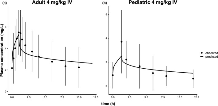
Model validation against observed data. Voriconazole plasma concentration‐time profiles for 4 mg/kg intravenous infusion dosing for adults (a) and children (b). The plots show the observed data (black dots) and the corresponding predictions from the adult and pediatric models (black lines). Error bars represent standard deviation.
The ODEs were declared in the [ODE] block as:
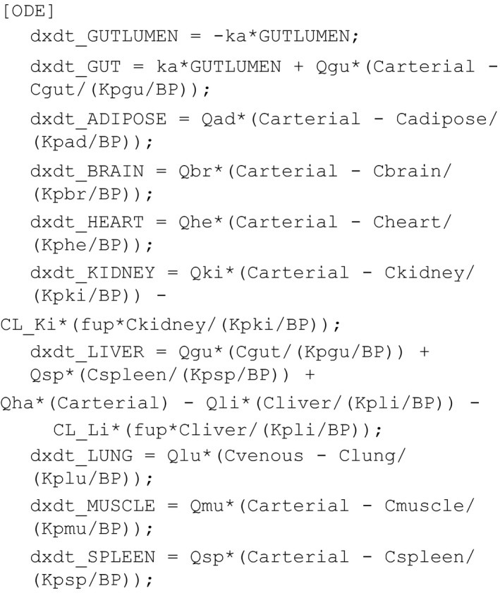
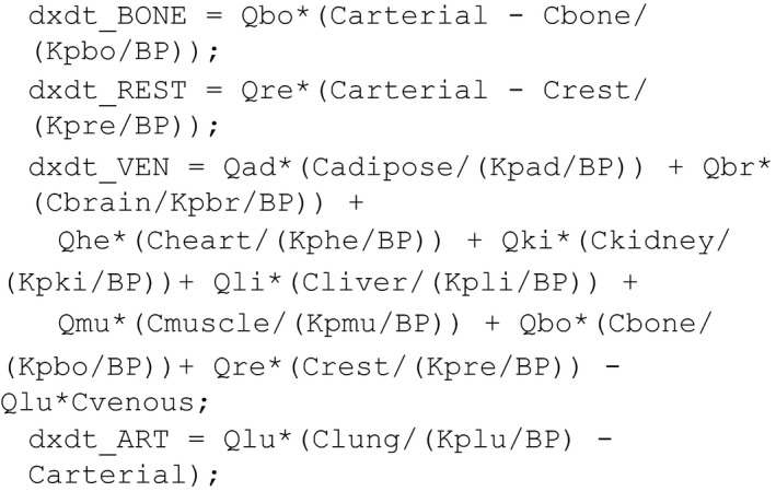
Voriconazole concentrations in different tissues were also declared in the [ODE] block because they were dependent on the state variables governed by the previous ODEs. For example, the muscle drug concentration was declared as:
double Cmuscle = MUSCLE/Vmu;
Organ volumes, blood flows, body weight, voriconazole absorption rate constant, unbound fraction, in vitro hepatic metabolism parameters, calculated Kp, and blood:plasma concentration ratio BP were directly declared in the [PARAM] block (see voriPBPK.cpp in the GitHub repository).
In the [MAIN] block, derived parameters included arterial and venous blood volumes, blood flow to the liver, volume and blood flow to the rest of the body compartment, and in vivo hepatic clearance as follows:
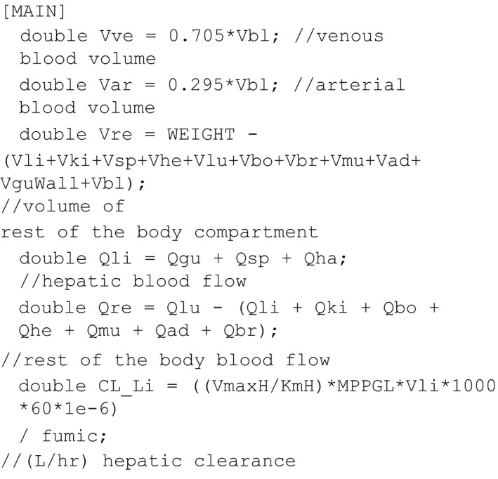
Finally, in the [TABLE] block, voriconazole plasma concentration can be captured to be part of the output as:
[TABLE] capture CP = Cvenous/BP;
Model validation
After model building, the following step would be to use the associated R script voriPBPK_script.R to compile the model and run simulations for model validation against the observed data. The script starts by cleaning up the working space and loading the necessary libraries. Then the adult model was compiled using the mread() function as follows:
modA <- mread("../model/voriPBPK")
This command compiles the adult model and saves it as modA object. The param() function was used to generate the pediatric model. First, a pedPhys object was created that was a named list of the curated pediatric physiological parameters19 and then a new pediatric model was generated by updating the adult model as follows:
modP <- param(modA, pedPhys)
Note that the updated parameter object needs to be a named list with the same parameter names as declared in the [PARAM] block.
Similarly, the K p values can be updated to reflect the calculated values using the Poulin and Theil method as previously described.20 To make this calculation process seamless and easily applicable to drugs other than voriconazole, an R script (calcKp_PT.R) was created that contains the function calcKp_PT(). This function takes any drug's physicochemical properties and returns a named list that can be directly used to update the PBPK model object. The function also needs fractional tissue composition data as another input. These data were digitized from the Poulin and Theil publication20 and saved as data/tissue_comp_PT.csv. For voriconazole, the K p updating was done by first reading in the tissue composition data, sourcing the calcKp_PT() function, calculating the K p values, and saving them as a named list Kp, then finally updating the model objects:
tissueComp <- read.csv("../data/tissue_comp_PT.csv") # tissue composition
source("calcKp_PT.R")
Kp <- calcKp_PT(logP=2.56, pKa=1.76, fup=0.42, BP=1, type=3, dat=tissueComp)
modA <- param(modA, Kp)
modP <- param(modP, Kp)
where the calcKp_PT() argument type was set to 3 for monoprotic base (see calcKp_PT.R for more details).
Next, simulations can be run to validate the model predictions against the digitized observed data from the Zane and Thakker publication15 (digitization was done using webplotdigitizer: https://automeris.io/WebPlotDigitizer/). The following two sets of clinical data were used for validation: (i) an adult 4 mg/kg intravenous infusion dose infused over an hour twice a day for a week and (ii) a pediatric 4 mg/kg intravenous infusion dose infused with a rate of 3 mg/kg/hour twice a day for a week. Steady‐state simulations were run for both populations under the same conditions as the observed data, and the simulation objects simA (for adults) and simP (for children) were created as follows:
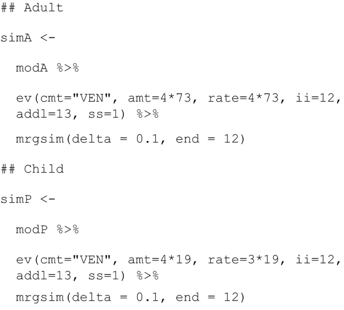
In the previous simulations, the function ev() was used to set the dosing events for the simulations as previously described. The simulation results were then plotted against the observed data and were shown to match well with the latter (Figure 3). As mentioned previously, the workflow in R could also be utilized to wrap the model objects within other R functions to run sensitivity analyses to pinpoint the most influential parameters (e.g., FME22 and sensitivity23 package functions) or to further tune the model predictions via parameter optimization.
QSP Application: Mitogen‐Activated Protein Kinase
Using the same approach, a QSP application is demonstrated in mrgsolve using the mitogen‐activated protein kinase (MAPK) model published by Kirouac et al.24 (Figure 4 ). The authors were interested in the clinical responses to therapy in colorectal cancer caused by a V600E/K mutation in the cytosolic kinase BRAF, which renders the kinase constitutively active and hence activates the downstream MEK and extracellular‐signal‐regulated kinase (ERK) signaling. BRAF and MEK inhibitors were found to be effective in V600E mutant melanoma, but these agents showed only a moderate effect in colorectal cancer. The purpose of the QSP model was to build a signaling cascade for MAPK (Figure 4 ) to assess the effect of introducing an ERK inhibitor as a monotherapy or in combination regimens with other agents on tumor size in colorectal cancer.24
Figure 4.
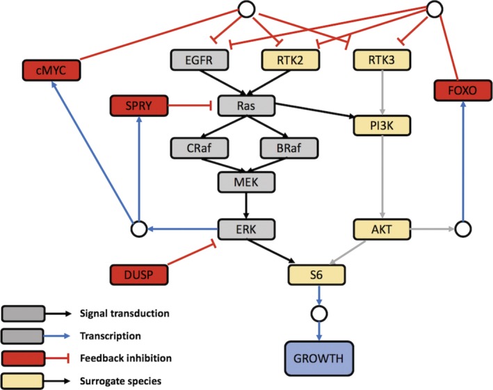
MAPK quantitative systems pharmacology model signaling network. Gray, red, and yellow nodes represent MAPK signaling pathway, regulatory feedback, and alternative signaling pathway components. Image was reproduced from24 under a Creative Commons Attribution 4.0 International License. DUSP, dual‐specificity phosphatase; EGFR, epidermal growth factor receptor; ERK, extracellular‐signal‐regulated kinase; FOXO, forkhead box protein; MAPK, mitogen‐activated protein kinase; PI3k, phosphatidylinositol‐3‐Kinase; RTK, receptor tyrosine kinase.
QSP model building in mrgsolve
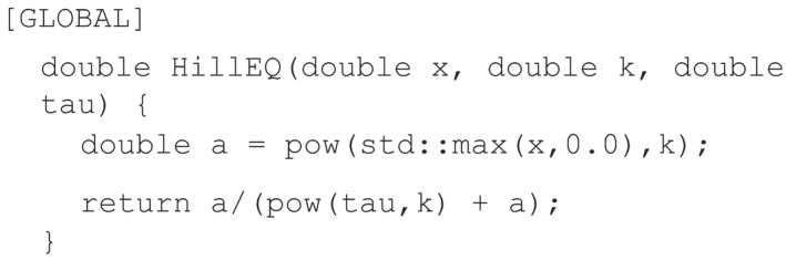
A mrgsolve model file was generated programmatically from the Systems Biology Markup Language file attached to the Kirouac et al. publication. The translation code was written in R and utilized an R interface to libSBML as linked from https://sbml.org. The translated model specification file model/mapkQSP.cpp in the associated GitHub repository contained the usual mrgsolve blocks [INIT], [PARAM], [ODE], and [TABLE], where the model compartments with their initial conditions, parameters, ODEs, and outputs were declared. A new [GLOBAL] block (see Table 1 ) was added to the specification file to define a Hill equation that would be used in the [ODE] block as follows:
The virtual population of 1,000 randomly sampled parameter values included as a supplement file in the Kirouac et al. publication was saved as data/s10vpop_pk.RDS. One set of these parameter values was used as a placeholder in the specification file [PARAM] block. For more details about the model structure and parameter values, please refer to mapkQSP.cpp in the associated GitHub repository.
Comparing different therapeutic combinations
The model was then used to compare the responses to different regimens of mono and combination drug therapies with and without an ERK inhibitor. The proposed drugs were the BRAF inhibitor vemurafenib (VEMU), the MEK inhibitor cobimetinib (COBI), the epidermal growth factor receptor antibody cetuximab (CETUX), and the ERK inhibitor GDC‐0994 (GDC). The clinical dosing regimens for COBI and GDC were daily dosing of 60 and 400 mg, respectively, with 21/7‐day on/off cycles, whereas for VEMU and CETUX the dosing was continuous 960 and 450 mg twice daily and weekly, respectively.24 These dosing regimens were implemented in the mapkQSP_script.R as follows:
# ERK inhibitor - GCD-994 (GDC) - Compartment 12
dataG <- ev(cmt = 12, amt = 400, ii = 1, addl = 20)
dataG <- seq(dataG, wait = 6, dataG)
# MEK inhibitor - cobimetinib (COBI) - Compartment 10
dataCO <- mutate(dataG, cmt=10, amt=60)
# EGFR inhibitor - cetuximab (CETUX) - Compartment 7
dataCE <- ev(cmt=7, amt=450, ii=7, addl=7)
# BRAF inhibitor - vemurafanib (VEMU) - Compartment 8
dataV <- ev(cmt=8, amt=960, ii=0.5, addl=120)
Two functions were created, (comb() and sim()), to combine dosing regimens and simulate, a data frame was then created to encompass all 16 possible combinations of the four drugs of interest, and finally the simulations were run given the full virtual population as follows:
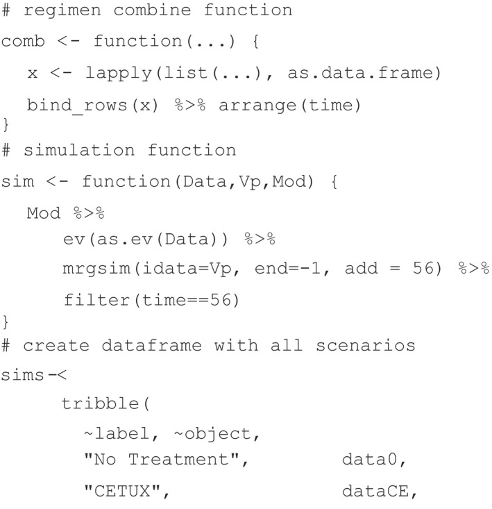
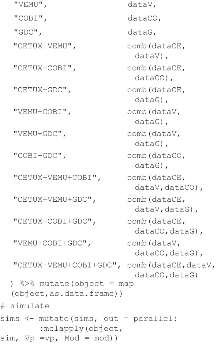
The end time for all simulations was 56 days (8 weeks) because this is the time when the tumor size response is assessed.24
The results for all simulations were summarized in Figure 5 , which was used as model verification as a reproduction of figure 6B from Kirouac et al.24 The figure depicts the noticeable impact of the ERK inhibitor GDC on tumor size either as a mono or combination therapy (red boxplots). The overall response rate (ORR) to GDC as a monotherapy or as a GDC + COBI combination therapy was quantified in the full virtual population vs. a subset of the population where tumor size was strongly dependent on MAPK signaling (represented by higher WOR parameter values). In the R/mrgsolve workflow, this was done as follows:
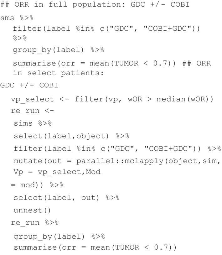
Figure 5.
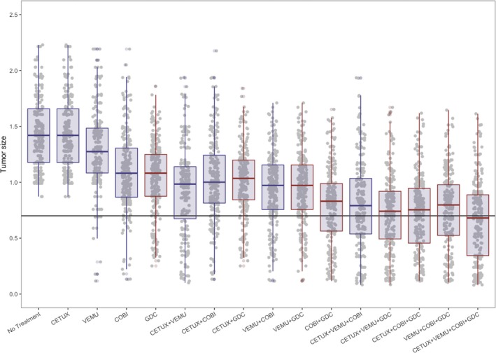
Effect of different drug combinations on tumor size. Normalized tumor size at week 8 is plotted against each of the 16 corresponding drug combinations. Gray dots and overlaid boxplots represent simulated tumor sizes with combinations containing GDC highlighted in red. Horizontal black line represents tumor size reduction of 30%. CETUX, cetuximab; COBI, cobimetinib; GDC, GDC‐0994; VEMU, vemurafenib.
Results traceably, and in an open‐source platform, reproduced the previously predicted ORR in the full population (14% and 35.2% for GDC and GDC+COBI, respectively), and a more significant ORR on the MAPK‐dependent subpopulation (28.7% and 70.5% for GDC and GDC+COBI, respectively) with the combination therapy approximating the ORR reached with BRAFV600E mutation melanoma patients (~70%).24 Complete reproduction of this example in mrgsolve is available in the following vignette: https://github.com/metrumresearchgroup/pbpk-qsp-mrgsolve/blob/master/docs/mapk_inhibitors_in_colorectal_cancer.md#translation
Funding
No funding was received for this work.
Conflict of Interest
The authors declared no competing interests for this work.
Supporting information
Supplementary Materials. mrgsolve model code for physiologically‐based pharmacokinetic and quantitative systems pharmacology example models.
References
- 1. Hindmarsh, A.C. ODEPACK, a systematized collection of ODE solvers In Scientific Computing, MACS Transactions on Scientific Computation, Vol. 1 (eds. Stepleman R.S. et al) 55–64 (North-Holland, Amsterdam, The Netherlands, 1983). [Google Scholar]
- 2. Eddelbuettel, D. Seamless R and C++ Integration With Rcpp (Springer Science & Business Media, Berlin, Germany, 2013). [Google Scholar]
- 3. Beal, S.L. & Sheiner, L.B. . NONMEM Users Guide (University of California, San Francisco, CA, 1992). [Google Scholar]
- 4. Eddelbuettel, D. & Sanderson, C. RcppArmadillo: accelerating R with high‐performance C linear algebra. Comput. Stat. Data Anal. 71, 1054–1063 (2014). [Google Scholar]
- 5. Pinheiro, J. , Bates, D. , DebRoy, S. & Sarkar, D. ; R Core Team . nlme: linear and nonlinear mixed effects models <https://CRAN.R-project.org/package=nlme> (2019).
- 6. Comets, E. , Lavenu, A. & Lavielle, M. Parameter estimation in nonlinear mixed effect models using saemix, an R implementation of the SAEM algorithm [internet]. J. Stat. Softw. 80 (2017). 10.18637/jss.v080.i03. [DOI] [Google Scholar]
- 7. Nyberg, J. , Ueckert, S. , Strömberg, E.A. , Hennig, S. , Karlsson, M.O. & Hooker, A.C. PopED: an extended, parallelized, nonlinear mixed effects models optimal design tool. Comput. Methods Programs Biomed. 108, 789–805 (2012). [DOI] [PubMed] [Google Scholar]
- 8. Bazzoli, C. , Retout, S. & Mentré, F. Design evaluation and optimisation in multiple response nonlinear mixed effect models: PFIM 3.0. Comput. Methods Programs Biomed. 98, 55–65 (2010). [DOI] [PubMed] [Google Scholar]
- 9. Wickham, H. tidyverse: easily install and load the “Tidyverse” <https://CRAN.R-project.org/package=tidyverse> (2017).
- 10. Lattice Nordhausen, K. Multivariate data visualization with R by Deepayan Sarkar. Int. Stat. Rev. 440(2008). 10.1111/j.1751-5823.2008.00062_5.x. [DOI] [Google Scholar]
- 11. R Core Team . R: A Language and Environment for Statistical Computing (R Foundation for Statistical Computing, Vienna, Austria, 2018). https://www.R-project.org/ [Google Scholar]
- 12. Gentzsch, W. Sun Grid Engine: towards creating a compute power grid Proceedings First IEEE/ACM International Symposium on Cluster Computing and the Grid. 10.1109/ccgrid.2001.923173 [DOI] [Google Scholar]
- 13. Chang, W. , Cheng, J. , Allaire, J.J. , Xie, Y. & McPherson, J. shiny: web application framework for R <https://CRAN.R-project.org/package=shiny> (2019)
- 14. Bache, S.M. & Wickham, H. . magrittr: a forward‐pipe operator for R https://CRAN.R-project.org/package=magrittr; (2014).
- 15. Zane, N.R. & Thakker, D.R. A physiologically based pharmacokinetic model for voriconazole disposition predicts intestinal first‐pass metabolism in children. Clin. Pharmacokinet. 53, 1171–1182 (2014). [DOI] [PubMed] [Google Scholar]
- 16. Thompson, M.D. & Beard, D.A. Development of appropriate equations for physiologically based pharmacokinetic modeling of permeability‐limited and flow‐limited transport. J. Pharmacokinet Pharmacodyn. 38, 405–421 (2011). [DOI] [PMC free article] [PubMed] [Google Scholar]
- 17. Zhuang, X. & Lu, C. PBPK modeling and simulation in drug research and development. Acta Pharm. Sin B. 6, 430–440 (2016). [DOI] [PMC free article] [PubMed] [Google Scholar]
- 18. Jones, H. & Rowland‐Yeo, K. Basic concepts in physiologically based pharmacokinetic modeling in drug discovery and development. CPT Pharmacometrics Syst Pharmacol. 2, e63 (2013). [DOI] [PMC free article] [PubMed] [Google Scholar]
- 19. Basic anatomical and physiological data for use in radiological protection: reference values. A report of age‐ and gender‐related differences in the anatomical and physiological characteristics of reference individuals. ICRP Publication 89. Ann. ICRP. 32, 5–265 (2002). [PubMed] [Google Scholar]
- 20. Poulin, P. & Theil, F.‐P. Prediction of pharmacokinetics prior to in vivo studies. 1. Mechanism‐based prediction of volume of distribution. J. Pharm. Sci. 91, 129–156 (2002). [DOI] [PubMed] [Google Scholar]
- 21. Yanni, S.B. , Annaert, P.P. , Augustijns, P. , Ibrahim, J.G. , Benjamin, D.K. Jr & Thakker, D.R. In vitro hepatic metabolism explains higher clearance of voriconazole in children versus adults: role of CYP2C19 and flavin‐containing monooxygenase 3. Drug Metab. Dispos. 38, 25–31 (2010). [DOI] [PMC free article] [PubMed] [Google Scholar]
- 22. Soetaert, K. & Petzoldt, T. Inverse modelling, sensitivity and Monte Carlo analysis in R using package FME. J. Stat. Softw. 33 (2010). 10.18637/jss.v033.i03. [DOI] [Google Scholar]
- 23. Iooss, B. et al Sensitivity: global sensitivity analysis of model outputs <https://CRAN.R-project.org/package=sensitivity> (2018).
- 24. Kirouac, D.C. et al Clinical responses to ERK inhibition in BRAFV600E‐mutant colorectal cancer predicted using a computational model. NPJ Syst. Biol. Appl. 3, 14 (2017). [DOI] [PMC free article] [PubMed] [Google Scholar]
Associated Data
This section collects any data citations, data availability statements, or supplementary materials included in this article.
Supplementary Materials
Supplementary Materials. mrgsolve model code for physiologically‐based pharmacokinetic and quantitative systems pharmacology example models.


