Hybrid Electron Microscopy Normal Mode Analysis with Scipion

Abstract

Hybrid Electron Microscopy Normal Mode Analysis (HEMNMA) method was introduced in 2014. HEMNMA computes normal modes of a reference model (an atomic structure or an electron microscopy map) of a molecular complex and uses this model and its normal modes to analyze single‐particle images of the complex to obtain information on its continuous conformational changes, by determining the full distribution of conformational variability from the images. An advantage of HEMNMA is a simultaneous determination of all parameters of each image (particle conformation, orientation, and shift) through their iterative optimization, which allows applications of HEMNMA even when the effects of conformational changes dominate those of orientational changes. HEMNMA was first implemented in Xmipp and was using MATLAB for statistical analysis of obtained conformational distributions and for fitting of underlying trajectories of conformational changes. A HEMNMA implementation independent of MATLAB is now available as part of a plugin of Scipion V2.0 (http://scipion.i2pc.es). This plugin, named ContinuousFlex, can be installed by following the instructions at https://pypi.org/project/scipion-em-continuousflex. In this article, we present this new HEMNMA software, which is user‐friendly, totally free, and open‐source.

Statement for a Broader Audience

This article presents Hybrid Electron Microscopy Normal Mode Analysis (HEMNMA) software that allows analyzing single‐particle images of a complex to obtain information on continuous conformational changes of the complex, by determining the full distribution of conformational variability from the images. The HEMNMA software is user‐friendly, totally free, open‐source, and available as part of ContinuousFlex plugin (https://pypi.org/project/scipion-em-continuousflex) of Scipion V2.0 (http://scipion.i2pc.es).

1. INTRODUCTION

Cryo‐electron microscopy (cryo‐EM) has become comparable to X‐ray crystallography with regards to the obtainable resolution of structures of biomolecular complexes, which are now increasingly determined at near‐atomic resolution.1, 2, 3, 4, 5, 6, 7, 8, 9, 10 No requirement for sample crystallization and the possibility to elucidate multiple conformations of a complex from the same sample are among the main advantages of cryo‐EM. Characterizing the different conformations that can coexist is essential for understanding how the complexes function and addressing their dynamics.

To achieve near‐atomic resolution of 3D reconstructions, the classical approach is to collect a large number of images of complexes (particles) at random and unknown orientations within a thin layer of vitreous ice, then, perform 2D and 3D classifications into an initially set number of classes and, finally, perform 3D reconstruction using only those particles that have the most consistent views and conformations (those that contribute to the highest‐resolution class averages) while removing all other particles.8, 9, 10, 11, 12, 13, 14 Such “selection” of particles may obscure information on a possibly larger conformational variability as some conformational states may be thrown away blindly instead of being elucidated. Therefore, non‐classification‐based methods are required to extract from images the full distribution of conformational variability (the so‐called conformational space or landscape in which the images are mapped) and to assemble 3D reconstructions from identified, more or less dense regions in this space (denser regions contain more frequent conformational states and less dense regions contain less frequent states). Such methods are necessary for studying continuous conformational changes of complexes (the concept including the possibility of unequally distributed conformers, e.g., possible existence of more stable conformers) and are referred to as continuous‐state methods. Many classification‐based methods (referred to as discrete‐state methods) can be found in the literature.15, 16, 17, 18, 19, 20, 21, 22, 23, 24, 25, 26, 27, 28 While the majority of the discrete‐state methods require that the number of classes is set initially, setting this number in some of the methods is less arbitrary as it is based on making a balance between intraclass and interclass variances after a statistical analysis of the data, typically using an eigenvector analysis of the covariance estimated from images or from volumes reconstructed from random subsets of images.18, 19, 21 The covariance eigenvectors estimation has also been introduced in the context of continuous conformational heterogeneity.29, 30 The latter methods are closely related to continuous‐state methods whose development started recently and are currently an active field of research.31, 32, 33, 34, 35, 36, 37

We introduced the continuous‐state method referred to as Hybrid Electron Microscopy Normal Mode Analysis (HEMNMA) in 2014.31, 32 HEMNMA computes normal modes of a reference model (an atomic structure or an EM map) of a molecular complex and uses this model and its normal modes to analyze single‐particle images of the complex iteratively in order to extract information on the full distribution of conformational variability from these images. In each iteration, HEMNMA aims at simultaneously solving both orientational and conformational heterogeneity of images using the reference model and its normal modes.

Although often considered as “model‐free,” the continuous‐state methods from other groups do use a model (e.g., the model used by Dashti et al.33 is EMDB‐1067 density map). This model is used to first solve the orientational heterogeneity of images, by determining the particle 3D orientation and 2D shift in each image assuming conformational homogeneity of images (e.g., the particle orientation and shift in each image can be determined by the standard projection matching of the image with the model). Then, the conformational heterogeneity of images is solved (i.e., the conformations are determined) using the image orientations and shifts determined in the previous step. These methods do not refine orientations and shifts when determining conformations, assuming that the effects of orientational changes dominate those of conformational changes so that each image can be associated with the correct orientation.

An advantage of HEMNMA is a simultaneous determination of all parameters of each image (particle conformation, orientation, and shift) through their iterative optimization, which allows applications of HEMNMA even when the effects of conformational changes dominate those of orientational changes. The simultaneous determination of the parameters is done by iterative matching of the image with projections of the reference model being deformed using a linear combination of normal modes (the conformation is estimated by determining the unknown coefficients of the linear combination, i.e., by determining the displacement amplitudes along normal modes). The reference model does not need to be an atomic‐resolution model and can also be an EM map. This EM map can be obtained by 3D reconstruction from combined data as if the data were conformationally homogeneous (e.g., by the so‐called random sample consensus approach that identifies the best EM maps from those reconstructed using random subsets of images and random image orientations,38 maximum likelihood optimization of a number of 3D reconstructions starting from random data subsets,39 or other methods40).

HEMNMA and other continuous‐state methods are fundamentally different from classification‐based (discrete‐state) methods. For instance, the discrete‐state method of Haselbach et al.27 uses standard Relion39 software for discrete classification of images into a number of 3D maps and standard principal component analysis (PCA) to cluster the maps. As similar classification‐based methods, it is prone to assigning images to lower‐noise density maps independently of whether or not the images belong there. For further reading on the different methods, the reader can refer to some of the recent methods reviews.41, 42, 43, 44, 45

The first version of HEMNMA was implemented in Xmipp46 and was using MATLAB for statistical analysis of obtained conformational distributions and for fitting of underlying trajectories of conformational changes.31, 32 A MATLAB‐independent version of HEMNMA was recently implemented in Scipion47 and is currently available as part of a plugin of Scipion V2.0 (http://scipion.i2pc.es). This plugin, named ContinuousFlex, can be installed by following the instructions at https://pypi.org/project/scipion-em-continuousflex. The new HEMNMA software is totally free and open‐source, and the new graphical interface is even more user‐friendly than the previous one. In this article, we present this new HEMNMA software.

2. HEMNMA WITHIN SCIPION: STEPS, PARAMETERS, AND GRAPHICAL INTERFACE

The steps to follow are listed in the HEMNMA menu on the left side of the Scipion project window and are numbered from 1 to 6. When the different steps are executed, a tree‐like structure of the project appears on the right side of the window, with each block corresponding to a step or a substep (Figures 1 and 2). In this section, we describe the steps (Steps 1–6), parameters, and graphical interface of HEMNMA. Each parameter is also described in the graphical interface, via a help message that can be displayed by clicking on the question mark next to the corresponding parameter field. The majority of the parameters are set to the values that usually produce good results. These default values are visible in the graphical interface and can be modified by the user. The parameters whose values are expected to be less frequently changed are hidden by default. By selecting “Advanced” as “Expert Level” mode (“Normal” is the default mode), the values of these “advanced” parameters can be visualized (the parameter names showing up on a grey background) and modified (e.g., Figure 3a).

Figure 1.

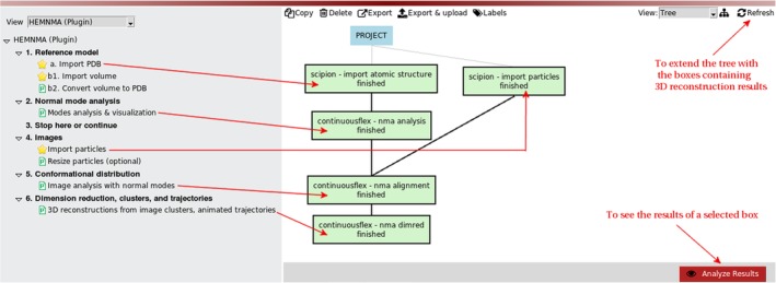
HEMNMA project tree for the case of analyzing images using an atomic structure as the reference model

Figure 2.

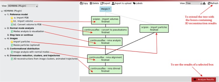
HEMNMA project tree for the case of analyzing images using a density volume as the reference model. The volume is converted into 3D Gaussian functions (the so‐called pseudoatoms)

Figure 3.

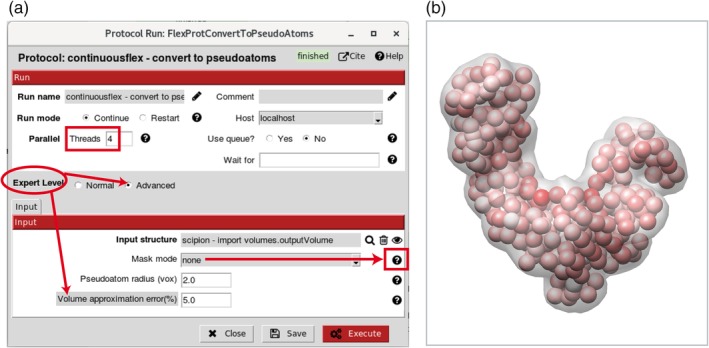
Volume‐to‐pseudoatoms conversion. (a) Dialog box. (b) Superposition of an input density volume (transparent grey) and its pseudoatomic representation [spheres where the amplitudes of Gaussian functions are color‐coded from white (smallest) to red (largest)]. In this example, the Gaussian‐function standard deviation (pseudoatom radius) and the desired volume approximation error are 2 voxels and 5%, respectively. The desired volume approximation error parameter is hidden by default (“Expert Level” is set to “Normal”) and can be visualized by setting “Expert Level” to “Advanced” (panel a). The volume‐to‐pseudoatoms conversion is parallelized using threads (parallel processes sharing the same memory) and the number of threads to use can be specified in the “Threads” field (panel a). The masking options to remove background noise from the input volume are explained in the help message under the corresponding question mark (panel a)

2.1. Step 1: Reference model

The reference model to import can be a PDB file with atomic coordinates or a density volume (e.g., an EM map or a simulated map from a PDB structure). Both import options are provided (Steps 1.a and 1.b1 in the project tree, Figures 1 and 2). Figures 1 and 2 show the project tree for an input atomic structure and for an input density volume, respectively. Before the next step, the input density volume must be converted into a PDB‐format file. We provide a tool for the volume conversion into a set of 3D Gaussian functions (Step 1.b2 in the project tree, Figure 2), the so‐called pseudoatoms,48 whose coordinates are written into a PDB file. More precisely, the conversion is performed so that the input density volume is represented with Gaussian functions of a given (input) standard deviation (“Pseudoatom radius” input parameter expressed in voxels), by minimizing the normalized volume approximation error48 to reach a given (input) value of this error (“Volume approximation error” parameter expressed in percent) (Figure 3). Note that the default value of the “Volume approximation error” parameter is 5%, which can be modified by first selecting “Advanced” as “Expert Level” mode to visualize the parameter (Figure 3a). Through this conversion procedure, some noise may be removed from the input density volume, as shown elsewhere.49 However, strong particle background noise should be removed using external tools or the masking procedures available in HEMNMA (“Mask mode” parameter in Figure 3a allows entering the name of a binary mask file or the threshold value below which the densities should be removed). For faster processing, the volume‐to‐pseudoatoms conversion was parallelized and should be run using several CPU threads (sharing the same memory). The number of threads can be specified via the “Threads” parameter (Figure 3a). The results of the volume‐to‐pseudoatoms conversion can be visualized with Chimera50 (Figure 3b) by clicking on the “Analyze Results” button in the project window (Figure 2).

After a displacement with normal modes, both an atomic reference model and a pseudoatomic reference model (from a reference density volume) are converted into a density volume whose projections are compared with images to determine the conformations in these images (Step 5). The higher the resolution of the reference model, the more accurate the normal modes and the conformational determination will be. Thus, the most accurate conformational determination is expected with input atomic models and high‐resolution EM maps.

The reference atomic model can be a full‐atomic model or a coarse‐grained model (e.g., containing Cα atoms only). The computation of normal modes (Step 2) requires information on the shape of the entire complex. An atomic model lacking a few small regions (e.g., disordered regions) may still be used as the reference model. If the atomic model lacks large portions of a complex and an EM map can be obtained for the entire complex, this EM map should be used as the reference model. An alternative reference model could be a hybrid model of the entire complex obtained by modeling the missing parts in the atomic model or the density volume computed from this hybrid model.

Classical, classification‐based approaches can be used to obtain a reference EM map for HEMNMA to analyze the entire heterogeneous set of images or an image subset with heterogeneity reduced through classification, as shown elsewhere.31 The use of classification‐based approaches before HEMNMA may be particularly useful in the case of combined discrete and continuous conformational heterogeneity (e.g., a mixture of flexible complexes bound and unbound with ligands).

There are no restrictions regarding the number of atoms in input PDB files or the size of input EM maps, except that the maps should have a cubic shape. There are no restrictions regarding the content of the atomic model, such as the presence of DNA, ligands, and so forth. However, in the case of a heterogeneous set of particles bound and unbound with ligands, it may be interesting to remove the ligand from the reference model, as shown elsewhere.31, 51

2.2. Step 2: Normal mode analysis

Normal modes of the atomic or pseudoatomic representation of the reference model (“Input structure” field in Figure 4a) are computed using Tirion's elastic network model.52 In this model, atoms or pseudoatoms interact if they are connected with elastic springs. The interaction cut‐off distance parameter determines how many atoms or pseudoatoms will be connected with elastic springs. The following two options exist for setting this value, via the “Cut‐off mode” parameter (Figure 4a): “absolute” and “relative.” If “absolute” is chosen for “Cut‐off mode” (unshown in Figure 4a), the interaction cut‐off distance value is an input parameter that should be set directly by the user (by setting the “Cut‐off distance” parameter, expressed in angstroms, which shows up only if “absolute” is chosen for “Cut‐off mode”). The default value of “Cut‐off distance” is 8 Å, which is the empirical recommended value for atomic structures. The “Cut‐off distance” value of 8 Å implies building an elastic network in which two atoms are connected with a spring (interact with each other) only if their distance is smaller than 8 Å. If “relative” is chosen for “Cut‐off mode,” the interaction cut‐off distance value is computed automatically based on a given (input) percentage of distances (“Cut‐off percentage” parameter expressed in percent, Figure 4a) that should be below this value. The default value of the “Cut‐off percentage” is 95%, which is the empirical recommended value for pseudoatomic structures. The “Cut‐off percentage” value of 95% implies building an elastic network in which two pseudoatoms are connected with a spring only if their distance is smaller than the one below which 95% of distances are. The larger the interaction cut‐off distance for a given complex, the more rigid the elastic network will be. A too‐large interaction cut‐off distance produces a too rigid elastic network, which can be detected and corrected by analyzing the normal‐mode animations with the provided graphical interface (normal mode analysis (NMA) results viewer in Figure 4b).

Figure 4.

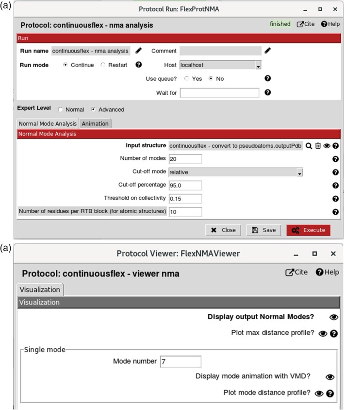
Normal mode analysis and visualization. (a) Dialog box (note that “Cut‐off mode” selected here is “relative” and that the interface allows selecting the cut‐off mode “absolute” as well). (b) Normal modes viewer allowing visualizing animations of normal modes (using “Display mode animation with VMD?” for the mode specified in “Mode number”) and checking their collectivities and scores (using “Display output Normal Modes?”)

Normal modes are computed by diagonalizing a square matrix of second derivatives of the potential energy function of the structure (Hessian matrix). One dimension of the Hessian matrix is three times the number of atoms or pseudoatoms. For faster Hessian diagonalization with input atomic structures (large Hessians due to large numbers of atoms), the structure is split into blocks of several residues, each block having six degrees of freedom (three rotations and three translations), which reduces the Hessian dimension to six times the number of blocks and is known as Rotation Translation Block (RTB) method.53 The number of residues per RTB block should be set by the user, and its default value in the graphical interface is 10 (Figure 4a). The larger the number of residues per block (i.e., the smaller the number of blocks), the faster the computation of normal modes and the more rigid the elastic network will be. A too large number of residues per block will produce a too rigid elastic network, which can be detected and corrected by analyzing the normal‐mode animations with the provided graphical interface (NMA results viewer, Figure 4b).

The number of computed normal modes is three times the number of pseudoatoms (for a pseudoatomic structure) or six times the number of RTB blocks (for an atomic structure). However, the number of modes written on the disk and animated should be set by the user (“Number of modes” parameter, Figure 4a). It is usually enough to save animations for 20–100 modes (e.g., the most relevant modes to experimentally observed conformational changes of low‐symmetry structures are generally among the first 10–20 lowest‐frequency non‐rigid‐body modes). The computed normal modes can be inspected by visualizing their animations, collectivities,54 and scores,32 via the NMA results viewer (Figure 4b) that can be obtained by clicking on the “Analyze Results” button in the project window. The collectivity54 indicates how much the atoms or pseudoatoms move together with a given mode. It is computed for the entire complex without differentiating between its domains and it is normalized between 1/N (maximally localized motion) and 1 (maximally collective motion), where N is the number of atoms or pseudoatoms. Highly collective low‐frequency modes have been shown to be functionally relevant.55, 56, 57, 58 Therefore, we also provide the score32 that combines the collectivity and frequency criteria, by penalizing the modes with higher frequencies and lower collectivities. The score is normalized between 1/M (highest collectivity and lowest frequency motion) and 1 (lowest collectivity and highest frequency motion), where M is the number of modes.

The list of modes, with their collectivities and scores, can be obtained using “Display output Normal Modes?” in the NMA results viewer (Figure 4b). The interface allows ordering the modes according to the increasing or decreasing values of the collectivity or score measures. The modes most relevant to the actual conformational change are expected to be among those with the lowest scores. The number of the lowest‐score modes to inspect should be larger in the case of highly symmetrical structures (e.g., icosahedral‐symmetry viruses) as highly collective modes may also exist at higher frequencies in such cases. To help the user decide which modes should certainly not be selected for the image analysis (Step 5), the modes with collectivities below 0.15 (very localized motions) are unchecked in the list of modes obtained via “Display output Normal Modes?” (Figure 4b). The value of 0.15 for this collectivity threshold can be modified by the user (“Threshold on collectivity” parameter, Figure 4a).

The motion trajectory along a normal mode is saved in a text file by concatenating the frames (in PDB format) of the coordinate displacement along this mode. The default number of frames is 10 and the default amplitude of the displacement along normal mode is 50 (these parameters can be modified via the “Animation” tab, unopened in Figure 4a). This trajectory file is animated with visual molecular dynamics (VMD),59 by selecting “Display mode animation with VMD?” and specifying the mode to be animated in the “Mode number” field (Figure 4b). VMD provides tools to save the motion trajectories in Animated GIF or MPEG movie formats that can be played with more standard movie players.

The modes can also be inspected by plotting the shifts of atoms (or pseudoatoms) along the specified mode and by plotting their maximum shifts over all modes via “Plot mode distance profile?” and “Plot max distance profile?,” respectively (Figure 4b). For instance, a too large shift of one or a very few atoms (or pseudoatoms) with respect to the shift of other atoms (or other pseudoatoms) is typically a sign that the value of the atomic (or pseudoatomic) interaction cut‐off distance used for computing normal modes is not optimal. In this case, normal modes should be recomputed using a modified value of this parameter.

2.3. Step 3: Information

At this step, entitled “Stop here or continue” in the HEMNMA menu (Figures 1 and 2), we remind the user that HEMNMA software may also be used for NMA only (the processing can be stopped after computing and analyzing normal modes at Step 2). The following steps should be performed if aiming at analyzing conformational heterogeneity in images using the normal modes computed in Step 2.

2.4. Step 4: Images

This step allows importing images that will be analyzed with normal modes. The images should have a square shape. They should have a power of 2 pixels in each dimension when using the so‐called “wavelet & splines” method for rigid‐body alignment in combination with the elastic alignment (see Step 5 for more information about the alignment methods). The larger the size of images, the longer the image analysis time will be. The image size can be reduced if the speed is an issue. The image size of 128 × 128 pixels is usually a good compromise.

2.5. Step 5: Conformational distribution

In this step, a combined elastic and rigid‐body alignment is performed between particle images and the reference model to calculate the parameters of orientation, translation, and elastic deformation (amplitudes of normal modes) of the reference model that best describe the given particle image.

Figure 5a shows the interface (“Input” tab) for selecting the images to be analyzed (“Input particles” parameter) and the normal modes to use for the image analysis (“Modes selection” parameter) from an entire list of computed normal modes (“Normal modes” parameter). The modes to use for the image analysis can be selected as the modes with the highest collectivities or least scores, with or without using previous knowledge about possible movements. The six lowest‐frequency modes (modes 1–6, where the index of the mode corresponds to the mode order according to the increasing frequency) describe rigid‐body movements of the structure and are often referred to as rigid‐body normal modes. These modes should not be selected because rigid‐body movements are taken into account through the iterative combined rigid‐body and elastic alignment, as explained in the next paragraph. Usually, this alignment is performed with 1–10 selected normal modes excluding modes 1–6.

Figure 5.

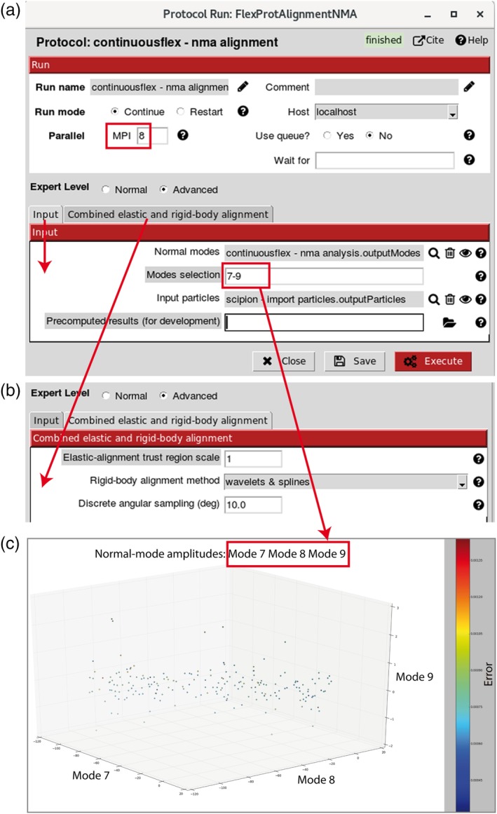
Image analysis with normal modes. (a) and (b) Two sections of the dialog box, regarding input (panel a) and alignment (panel b). (c) An example of visualization of image analysis results in three dimensions (amplitudes along three normal modes). The image analysis task is parallelized using MPI protocol and the number of MPI cores (parallel processes that do not necessarily share the same memory) can be specified in the MPI field (panel a). In panel b, the default choice for the “Rigid‐body alignment method” is “wavelets & splines” (the alternative method is “projection matching”) and the elastic alignment is performed by Powell's trust region method. In panel c, each point corresponds to a particle image with assigned orientations, translations, and normal‐mode displacement amplitudes with respect to the reference model (close points correspond to similar conformations and vice versa)

The interface for setting the parameters of the combined elastic and rigid‐body alignment is shown in Figure 5b (“Combined elastic and rigid‐body alignment” tab). We use Powell's optimization (more precisely, Powell's trust region method60) to iteratively estimate the elastic deformation (normal‐mode amplitudes) of the reference model by maximizing the similarity between the particle image and the best matching projection of the deformed model (objective function, in optimization terminology). In each iteration of Powell's method, an estimate of the normal‐mode amplitudes is used to displace the atoms or the pseudoatoms along with normal modes and the obtained, elastically deformed structure is converted into a density volume that is then rigid‐body aligned with the particle image. The rigid‐body alignment allows the determination of the orientation and translation parameters (rigid‐body parameters) and the objective‐function evaluation that is then used to better estimate the normal‐mode amplitudes (elastic deformation parameters) for the next iteration of Powell's method.

The values of the parameters of Powell's method are set internally in the code and are not modifiable via the interface except for the scaling factor of the initial trust‐region radius (“Elastic‐alignment trust region scale” parameter in Figure 5b). The default value of the scaling factor is 1, which generally works well. When expecting larger conformational changes, it may be interesting to increase the scaling factor (typically to a value between 1 and 2). The rigid‐body alignment can be performed using one of the following two methods: (a) “projection matching” that stands for the standard reference‐library‐based (discrete) projection matching in real space (faster but less accurate method); and (b) “wavelets & splines” that stands for a discrete projection matching in wavelet space61 followed by a continuous matching in 3D Fourier space based on spline interpolation62 (slower but more accurate method; in particular, more robust to noise). The default choice is “wavelets & splines” (“Rigid‐body alignment method” in Figure 5b). The angular sampling step61 for the reference projection library computation is 10° by default and can be modified via the interface (“Discrete angular sampling” parameter expressed in degrees, Figure 5b).

This combined rigid‐body and elastic alignment is the task that requires the most computation. Therefore, it was message passing interface (MPI) parallelized to simultaneously process N particle images using N MPI cores on CPU computers, clusters or supercomputers. The user specifies the number of MPI cores to be used (“MPI” parameter in Figure 5a). On an Intel Xeon CPU at 2.9 GHz, the analysis of one particle image of size 128 × 128 pixels with 3, 6, and 9 normal modes may, respectively, take 2, 5, and 10 min when using “projection matching” rigid‐body alignment and 5, 13, and 25 min when using “wavelets & splines” rigid‐body alignment.

Normal‐mode amplitudes resulting from the image analysis with normal modes can be visualized in one dimension (histogram) as well as in two or three dimensions (Figure 5c). Points in a 2D and 3D space correspond to images with assigned orientations, translations, and normal‐mode displacement amplitudes with respect to the reference model. Close points in this space correspond to similar conformations and vice versa.

2.6. Step 6: Dimension reduction, clusters, and trajectories

The normal‐mode displacement amplitudes obtained by image analysis in Step 5 can be projected onto a space of lower dimension (1D, 2D, or 3D) (Figure 6), using the technique of PCA or one of several other dimension reduction techniques.63 To perform the dimension reduction, the user specifies the conformational distribution to be analyzed (the image analysis results obtained in Step 5), the desired lower dimension, and one of the available linear or nonlinear dimensionality reduction techniques via “Conformational distribution,” “Reduced dimension,” and “Dimensionality reduction method” fields, respectively (Figure 6a). The “Extra params” field (Figure 6a) allows modifying the parameters of the dimensionality reduction techniques (the parameters and their default values are listed in the help message linked to the “Dimensionality reduction method” field). The available dimensionality reduction techniques are PCA, Kernel PCA, Probabilistic PCA, Local Tangent Space Alignment (LTSA), Linear LTSA, Diffusion Map, Linearity Preserving Projection, Laplacian Eigenmap, Hessian Locally Linear Embedding, Stochastic Proximity Embedding, and Neighborhood Preserving Embedding.63 The dimension reduction viewer (Figure 6b) can be obtained by clicking on “Analyze Results” button in the project window. It allows displaying the axes of the low‐dimensional space (Figure 6c) specified via the “Display normal‐mode amplitudes in the low‐dimensional space” field (Figure 6b). Also, the dimension reduction viewer (Figure 6b) allows opening the tool for making animations (“Trajectories Tool,” Figure 7a) and the tool for computing 3D reconstructions (“Clustering Tool,” Figure 8a).

Figure 6.

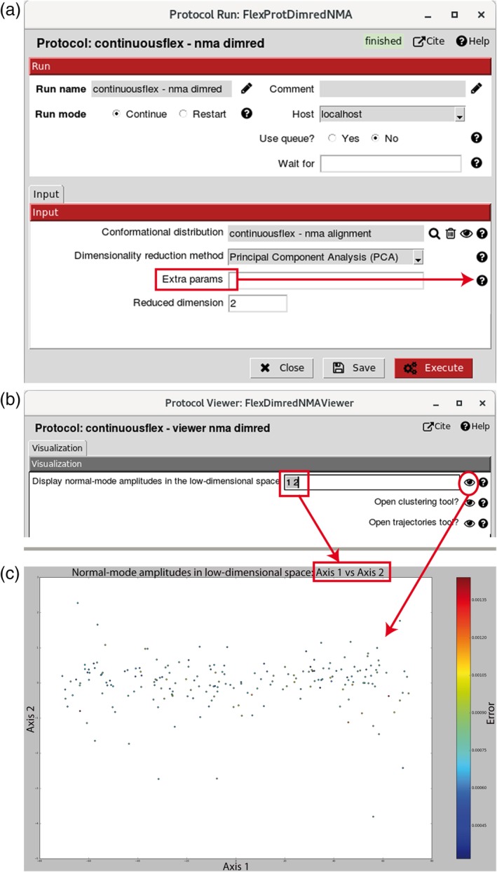
Dimension reduction. (a) Dialog box for projecting normal‐mode amplitudes computed by image analysis onto a space of lower dimension using PCA (here, 2 in “Reduced dimension” means projecting onto a 2D space) or one of several other dimension reduction methods selected via “Dimensionality reduction method” (the default values of parameters of these methods are provided in the help message displayable by clicking on the corresponding question mark). (b) Dimension reduction viewer allowing visualizing normal‐mode amplitudes in the low‐dimensional space (here, a 2D space specified by axes 1 and 2) as well as opening the clustering (grouping) and trajectories tools. (c) Example of projecting normal‐mode amplitudes onto a low‐dimensional space (here, 2D space specified in panel b). In panel a, the methods available for the dimension reduction are PCA, Kernel PCA, Probabilistic PCA, Local Tangent Space Alignment (LTSA), Linear LTSA, Diffusion Map, Linearity Preserving Projection, Laplacian Eigenmap, Hessian Locally Linear Embedding, Stochastic Proximity Embedding, and Neighborhood Preserving Embedding

Figure 7.

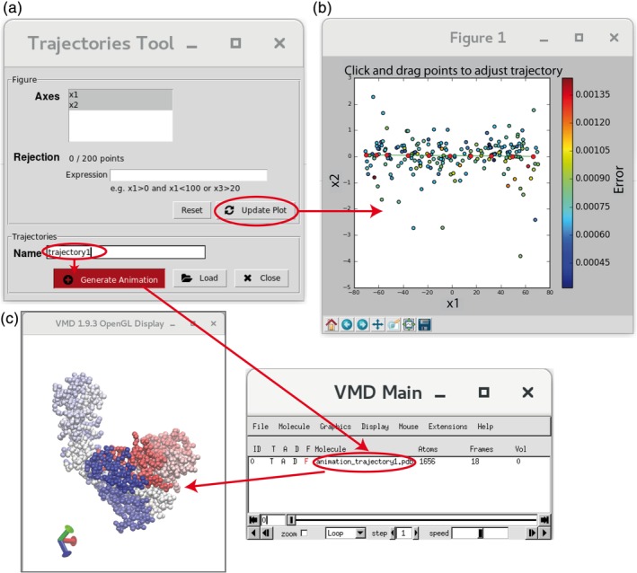
Animations after image analysis. (a) Trajectories Tool. (b) Example of trajectory (10 red points, see the text for more details). (c) Trajectory animation using VMD

Figure 8.

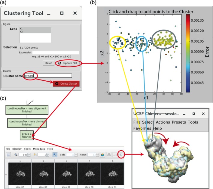
3D reconstructions after image analysis. (a) Clustering Tool for grouping close points (images with similar conformations). (b) Example of selecting a group of points (circled in yellow) for 3D reconstruction. (c) Chimera superposition of three 3D reconstructions (yellow, cyan, and gray isosurfaces) from the corresponding groups of images denoted in panel b (points surrounded by yellow, cyan, and gray ellipses, panel b), with the most dominant motion shown by red arrows. The group of points saved using the “Create Cluster” button (panel a) appears as a new box in the project tree (panel c), possibly after using the “Refresh” button from the project window. The saved group of points can be inspected using the “Analyze Results” button from the project window, which shows images in this group (not shown here) and slices of the volume reconstructed from these images (panel c). The volume isosurface can be visualized by clicking on the Chimera icon in the slices display menu (panel c)

While the advantage of nonlinear dimensionality reduction techniques is better suitability to nonlinear manifold data representations, the advantage of linear dimensionality reduction techniques (PCA, Linear LTSA, Linearity Preserving Projection, Probabilistic PCA, and Neighborhood Preserving Embedding) is that they allow mapping from the low‐dimensional space back to the original space. HEMNMA uses this property to generate animated trajectories of conformational changes. More precisely, the “Trajectories Tool” (Figure 7a) allows recording and visualizing the displacement of the reference model in the low‐dimensional space. The specification of the displacement trajectory to be animated requires the user's interaction. The outlier data points can be removed by providing logical (Boolean) expressions (“Expression” field in Figure 7a). The trajectory is specified by the coordinates of 10 points in the low‐dimensional space (red points in Figure 7b). The user may select all of these 10 points (by clicking on the plot to select each point) or eight points may be automatically placed on a line between two points selected by the user (the first and last points of the trajectory). The position of the initially placed points may be changed by dragging the points. As in the case of animations of normal modes in Step 2, the trajectory is saved in a text file by concatenating the PDB‐format frames of the coordinate displacement. The trajectory can be animated with VMD (Figure 7c) or saved with VMD in Animated GIF or MPEG movie formats for playing with other movie players.

Additionally, conformational changes can be analyzed in terms of 3D reconstructions from images in the low‐dimensional space. “Clustering Tool” (Figure 8a) allows making groups of close points (Figure 8b), corresponding to images with similar conformational states, and computing 3D reconstructions from these groups (Figure 8c). A group of points is specified by providing logical (Boolean) expressions (“Expression” field in Figure 8a) or by clicking on the plot and dragging to add points to the group. Each point in the selected group of points is denoted by a yellow circle (Figure 8b). Clicking on the “Create Cluster” button (Figure 8a) saves the selected group of points and performs 3D reconstruction from this group. The saved group can be inspected by displaying the 3D reconstruction results (slices and isosurface of the reconstructed volume, Figure 8c) and the images present in the group (the images are not shown in Figure 8). HEMNMA uses a fast Fourier‐space method for 3D reconstruction from the selected group of points. The 3D reconstruction can be performed with other reconstruction methods (available in Scipion or other software packages), using the output metadata (text) file with the rigid‐body and elastic alignment parameters corresponding to the selected group of points. The 3D reconstructions represent the average states from the corresponding groups of images. One should make as homogeneous groups of points as possible with a sufficient number of points per group in order to obtain high‐resolution 3D reconstructions (note that the example in Figure 8b does not show the most optimal grouping of points).

As explained, HEMNMA provides a full conformational variability landscape before grouping images into 3D reconstructions (images with similar conformations on the landscape). As such, HEMNMA can detect the conformations and motions that are undetectable with traditional classification‐based approaches, which was extensively studied elsewhere.31

3. PERSPECTIVES

A full description of conformational heterogeneity is important for both biology and drug design. Cryo‐EM has been under continuous development since its beginning (early '80s), which was even accelerated with the latest instrumental developments including direct electron detector devices (DDD cameras). Allowing a routine near‐atomic resolution of structures and a routine full description of conformational variability are currently two main challenges. Indeed, the recent cryo‐EM advances such as DDD cameras, phase plates, and sample motion correction have reduced noise and improved contrast in images, which makes elucidation of conformations from images more accurate. Methods for a full description of continuous conformational variability are being developed. However, these methods will need to be more efficient and user‐friendly to allow routine use of cryo‐EM for such studies. HEMNMA is a user‐friendly software that has been developed for determining the full distribution of continuous conformational variability from cryo‐EM images. Still, HEMNMA needs to be made faster in order to allow an efficient high‐resolution description of this variability. For instance, the analysis of 10⁴ particle images based on the elastic alignment with six normal modes and the “wavelets & splines” rigid‐body alignment may take 17 hr using 128 MPI cores on 2.9 GHz Intel Xeon CPUs, which means that the analysis of 10⁶ particle images would require around 70 days of use of the same 128 MPI cores. To get a high‐resolution description of the full conformational landscape of a complex, several millions of particle images would need to be analyzed. A combination of HEMNMA with a deep learning approach will be implemented in the future to speed up the processing of such large numbers of particle images.

HEMNMA is well suited to compact‐support particle shapes and may be adapted to deal with helical symmetry particles in the future.

Harastani M, Sorzano COS, Jonić S. Hybrid Electron Microscopy Normal Mode Analysis with Scipion. Protein Science. 2020;29:223–236. 10.1002/pro.3772

REFERENCES

- 1. Zhang X, Settembre E, Xu C, et al. Near‐atomic resolution using electron cryomicroscopy and single‐particle reconstruction. Proc Natl Acad Sci U S A. 2008;105:1867–1872. [DOI] [PMC free article] [PubMed] [Google Scholar]
- 2. Yu X, Jin L, Zhou ZH. 3.88 a structure of cytoplasmic polyhedrosis virus by cryo‐electron microscopy. Nature. 2008;453:415–419. [DOI] [PMC free article] [PubMed] [Google Scholar]
- 3. Liao M, Cao E, Julius D, Cheng Y. Structure of the trpv1 ion channel determined by electron cryo‐microscopy. Nature. 2013;504:107–112. [DOI] [PMC free article] [PubMed] [Google Scholar]
- 4. Bai XC, Yan C, Yang G, et al. An atomic structure of human gamma‐secretase. Nature. 2015;525:212–217. [DOI] [PMC free article] [PubMed] [Google Scholar]
- 5. Bartesaghi A, Merk A, Banerjee S, et al. 2.2 a resolution cryo‐em structure of beta‐galactosidase in complex with a cell‐permeant inhibitor. Science. 2015;348:1147–1151. [DOI] [PMC free article] [PubMed] [Google Scholar]
- 6. Nguyen TH, Galej WP, Bai XC, et al. Cryo‐em structure of the yeast u4/u6.U5 tri‐snrnp at 3.7 a resolution. Nature. 2016;530:298–302. [DOI] [PMC free article] [PubMed] [Google Scholar]
- 7. Natchiar SK, Myasnikov AG, Kratzat H, Hazemann I, Klaholz BP. Visualization of chemical modifications in the human 80s ribosome structure. Nature. 2017;551:472–477. [DOI] [PubMed] [Google Scholar]
- 8. Zhang J, Ma J, Liu D, et al. Structure of phycobilisome from the red alga griffithsia pacifica. Nature. 2017;551:57–63. [DOI] [PubMed] [Google Scholar]
- 9. Liu Y, Gonen S, Gonen T, Yeates TO . Near‐atomic cryo‐em imaging of a small protein displayed on a designed scaffolding system. Proc Natl Acad Sci U S A. 2018;115:3362–3367. [DOI] [PMC free article] [PubMed] [Google Scholar]
- 10. Fan X, Wang J, Zhang X, et al. Single particle cryo‐em reconstruction of 52 kDa streptavidin at 3.2 angstrom resolution. Nat Commun. 2019;10:2386. [DOI] [PMC free article] [PubMed] [Google Scholar]
- 11. Khatter H, Myasnikov AG, Natchiar SK, Klaholz BP. Structure of the human 80s ribosome. Nature. 2015;520:640–645. [DOI] [PubMed] [Google Scholar]
- 12. He Y, Yan C, Fang J, et al. Near‐atomic resolution visualization of human transcription promoter opening. Nature. 2016;533:359–365. [DOI] [PMC free article] [PubMed] [Google Scholar]
- 13. Banerjee S, Bartesaghi A, Merk A, et al. 2.3 a resolution cryo‐em structure of human p97 and mechanism of allosteric inhibition. Science. 2016;351:871–875. [DOI] [PMC free article] [PubMed] [Google Scholar]
- 14. Abeyrathne PD, Koh CS, Grant T, Grigorieff N, Korostelev AA. Ensemble cryo‐em uncovers inchworm‐like translocation of a viral ires through the ribosome. Elife. 2016;5:e14874. [DOI] [PMC free article] [PubMed] [Google Scholar]
- 15. van Heel M, Stoffler‐Meilicke M. Characteristic views of E. coli and B. stearothermophilus 30s ribosomal subunits in the electron microscope. EMBO J. 1985;4:2389–2395. [DOI] [PMC free article] [PubMed] [Google Scholar]
- 16. Penczek PA, Frank J, Spahn CM. A method of focused classification, based on the bootstrap 3d variance analysis, and its application to ef‐g‐dependent translocation. J Struct Biol. 2006;154:184–194. [DOI] [PubMed] [Google Scholar]
- 17. Scheres SH, Gao H, Valle M, et al. Disentangling conformational states of macromolecules in 3d‐em through likelihood optimization. Nat Methods. 2007;4:27–29. [DOI] [PubMed] [Google Scholar]
- 18. Elad N, Clare DK, Saibil HR, Orlova EV. Detection and separation of heterogeneity in molecular complexes by statistical analysis of their two‐dimensional projections. J Struct Biol. 2008;162:108–120. [DOI] [PubMed] [Google Scholar]
- 19. Simonetti A, Marzi S, Myasnikov AG, et al. Structure of the 30s translation initiation complex. Nature. 2008;455:416–420. [DOI] [PubMed] [Google Scholar]
- 20. Sorzano COS, Bilbao‐Castro JR, Shkolnisky Y, et al. A clustering approach to multireference alignment of single‐particle projections in electron microscopy. J Struct Biol. 2010;171:197–206. [DOI] [PMC free article] [PubMed] [Google Scholar]
- 21. Penczek PA, Kimmel M, Spahn CM. Identifying conformational states of macromolecules by Eigen‐analysis of resampled cryo‐em images. Structure. 2011;19:1582–1590. [DOI] [PMC free article] [PubMed] [Google Scholar]
- 22. Scheres SH. A bayesian view on cryo‐em structure determination. J Mol Biol. 2012;415:406–418. [DOI] [PMC free article] [PubMed] [Google Scholar]
- 23. Lyumkis D, Brilot AF, Theobald DL, Grigorieff N. Likelihood‐based classification of cryo‐em images using frealign. J Struct Biol. 2013;183:377–388. [DOI] [PMC free article] [PubMed] [Google Scholar]
- 24. Fischer N, Neumann P, Konevega AL, et al. Structure of the E. coli ribosome‐ef‐tu complex at <3 a resolution by cs‐corrected cryo‐em. Nature. 2015;520:567–570. [DOI] [PubMed] [Google Scholar]
- 25. Scheres SHW. Processing of structurally heterogeneous cryo‐em data in relion Methods in enzymology. Ed. Crowther RA. Academic Press, 2016; p. 125–157 Chap. 6. [DOI] [PubMed] [Google Scholar]
- 26. Punjani A, Rubinstein JL, Fleet DJ, Brubaker MA. Cryosparc: Algorithms for rapid unsupervised cryo‐em structure determination. Nat Methods. 2017;14:290–296. [DOI] [PubMed] [Google Scholar]
- 27. Haselbach D, Komarov I, Agafonov DE, et al. Structure and conformational dynamics of the human spliceosomal b(act) complex. Cell. 2018;172(454–464):e411. [DOI] [PubMed] [Google Scholar]
- 28. Grant T, Rohou A, Grigorieff N. Cistem, user‐friendly software for single‐particle image processing. Elife. 2018;7:e35383. [DOI] [PMC free article] [PubMed] [Google Scholar]
- 29. Katsevich E, Katsevich A, Singer A. Covariance matrix estimation for the cryo‐em heterogeneity problem. SIAM J Imaging Sci. 2015;8:126–185. [DOI] [PMC free article] [PubMed] [Google Scholar]
- 30. Tagare HD, Kucukelbir A, Sigworth FJ, Wang H, Rao M. Directly reconstructing principal components of heterogeneous particles from cryo‐em images. J Struct Biol. 2015;191:245–262. [DOI] [PMC free article] [PubMed] [Google Scholar]
- 31. Jin Q, Sorzano CO, de la Rosa‐Trevin JM, et al. Iterative elastic 3d‐to‐2d alignment method using normal modes for studying structural dynamics of large macromolecular complexes. Structure. 2014;22:496–506. [DOI] [PubMed] [Google Scholar]
- 32. Sorzano CO, de la Rosa‐Trevin JM, Tama F, Jonic S. Hybrid electron microscopy normal mode analysis graphical interface and protocol. J Struct Biol. 2014;188:134–141. [DOI] [PubMed] [Google Scholar]
- 33. Dashti A, Schwander P, Langlois R, et al. Trajectories of the ribosome as a brownian nanomachine. Proc Natl Acad Sci U S A. 2014;111:17492–17497. [DOI] [PMC free article] [PubMed] [Google Scholar]
- 34. Frank J, Ourmazd A. Continuous changes in structure mapped by manifold embedding of single‐particle data in cryo‐em. Methods. 2016;100:61–67. [DOI] [PMC free article] [PubMed] [Google Scholar]
- 35. Anden J, Singer A. Structural variability from noisy tomographic projections. SIAM J Imaging Sci. 2018;11:1441–1492. [DOI] [PMC free article] [PubMed] [Google Scholar]
- 36. Dashti A, Hail DB, Mashayekhi G, et al. Conformational dynamics and energy landscapes of ligand binding in ryr1, bioRxiv 167080.
- 37. Lederman RR, Singer A Continuously heterogeneous hyper‐objects in cryo‐em and 3‐d movies of many temporal dimensions, arXiv 1704.02899.
- 38. Vargas J, Alvarez‐Cabrera AL, Marabini R, Carazo JM, Sorzano CO. Efficient initial volume determination from electron microscopy images of single particles. Bioinformatics. 2014;30:2891–2898. [DOI] [PubMed] [Google Scholar]
- 39. Scheres SH. Relion: Implementation of a bayesian approach to cryo‐em structure determination. J Struct Biol. 2012;180:519–530. [DOI] [PMC free article] [PubMed] [Google Scholar]
- 40. Reboul CF, Eager M, Elmlund D, Elmlund H. Single‐particle cryo‐em‐improved ab initio 3d reconstruction with simple/prime. Protein Sci. 2018;27:51–61. [DOI] [PMC free article] [PubMed] [Google Scholar]
- 41. Klaholz BP. Structure sorting of multiple macromolecular states in heterogeneous cryo‐em samples by 3d multivariate statistical analysis. Open J Stat. 2015;5:820–836. [Google Scholar]
- 42. Jonic S. Computational methods for analyzing conformational variability of macromolecular complexes from cryo‐electron microscopy images. Curr Opin Struct Biol. 2017;43:114–121. [DOI] [PubMed] [Google Scholar]
- 43. Cossio P, Hummer G. Likelihood‐based structural analysis of electron microscopy images. Curr Opin Struct Biol. 2018;49:162–168. [DOI] [PubMed] [Google Scholar]
- 44. Sorzano COS, Jimenez A, Mota J, et al. Survey of the analysis of continuous conformational variability of biological macromolecules by electron microscopy. Acta Crystallogr. 2019;F75:19–32. [DOI] [PMC free article] [PubMed] [Google Scholar]
- 45. Serna M. Hands on methods for high resolution cryo‐electron microscopy structures of heterogeneous macromolecular complexes. Front Mol Biosci. 2019;6:33–33. [DOI] [PMC free article] [PubMed] [Google Scholar]
- 46. Sorzano CO, Marabini R, Velazquez‐Muriel J, et al. Xmipp: A new generation of an open‐source image processing package for electron microscopy. J Struct Biol. 2004;148:194–204. [DOI] [PubMed] [Google Scholar]
- 47. de la Rosa‐Trevin JM, Quintana A, del Cano L, et al. Scipion: A software framework toward integration, reproducibility and validation in 3d electron microscopy. J Struct Biol. 2016;195:93–99. [DOI] [PubMed] [Google Scholar]
- 48. Jonic S, Sorzano COS. Coarse‐graining of volumes for modeling of structure and dynamics in electron microscopy: Algorithm to automatically control accuracy of approximation. IEEE J Sel Top Signal Process. 2016;10:161–173. [Google Scholar]
- 49. Jonic S, Vargas J, Melero R, Gomez‐Blanco J, Carazo JM, Sorzano CO. Denoising of high‐resolution single‐particle electron‐microscopy density maps by their approximation using three‐dimensional Gaussian functions. J Struct Biol. 2016;194:423–433. [DOI] [PubMed] [Google Scholar]
- 50. Pettersen EF, Goddard TD, Huang CC, et al. UCSF chimera—A visualization system for exploratory research and analysis. J Comput Chem. 2004;25:1605–1612. [DOI] [PubMed] [Google Scholar]
- 51. Sanchez Sorzano CO, Alvarez‐Cabrera AL, Kazemi M, Carazo JM, Jonic S. Structmap: Elastic distance analysis of electron microscopy maps for studying conformational changes. Biophys J. 2016;110:1753–1765. [DOI] [PMC free article] [PubMed] [Google Scholar]
- 52. Tirion MM. Large amplitude elastic motions in proteins from a single‐parameter, atomic analysis. Phys Rev Lett. 1996;77:1905–1908. [DOI] [PubMed] [Google Scholar]
- 53. Tama F, Gadea FX, Marques O, Sanejouand YH. Building‐block approach for determining low‐frequency normal modes of macromolecules. Proteins. 2000;41:1–7. [DOI] [PubMed] [Google Scholar]
- 54. Bruschweiler R. Collective protein dynamics and nuclear spin relaxation. J Chem Phys. 1995;102:3396–3403. [Google Scholar]
- 55. Delarue M, Dumas P. On the use of low‐frequency normal modes to enforce collective movements in refining macromolecular structural models. Proc Natl Acad Sci U S A. 2004;101:6957–6962. [DOI] [PMC free article] [PubMed] [Google Scholar]
- 56. Suhre K, Navaza J, Sanejouand YH. Norma: A tool for flexible fitting of high‐resolution protein structures into low‐resolution electron‐microscopy‐derived density maps. Acta Crystallogr D. 2006;62:1098–1100. [DOI] [PubMed] [Google Scholar]
- 57. Tama F, Miyashita O, Brooks CL 3rd. Flexible multi‐scale fitting of atomic structures into low‐resolution electron density maps with elastic network normal mode analysis. J Mol Biol. 2004;337:985–999. [DOI] [PubMed] [Google Scholar]
- 58. Wang Y, Rader AJ, Bahar I, Jernigan RL. Global ribosome motions revealed with elastic network model. J Struct Biol. 2004;147:302–314. [DOI] [PubMed] [Google Scholar]
- 59. Humphrey W, Dalke A, Schulten K. VMD: Visual molecular dynamics. J Mol Graph. 1996;14(33–38):27–38. [DOI] [PubMed] [Google Scholar]
- 60. Powell MJD. Uobyqa: Unconstrained optimization by quadratic approximation. Math Program. 2002;92:555–582. [Google Scholar]
- 61. Sorzano CO, Jonic S, El‐Bez C, et al. A multiresolution approach to orientation assignment in 3d electron microscopy of single particles. J Struct Biol. 2004;146:381–392. [DOI] [PubMed] [Google Scholar]
- 62. Jonic S, Sorzano CO, Thevenaz P, El‐Bez C, De Carlo S, Unser M. Spline‐based image‐to‐volume registration for three‐dimensional electron microscopy. Ultramicroscopy. 2005;103:303–317. [DOI] [PubMed] [Google Scholar]
- 63. Van der Maaten L, Postma E, Van den Herik J. Dimensionality reduction: A comparative review. Tilburg University Technical Report, TiCC‐TR 2009‐005, 2009. [Google Scholar]