Nonparametric competing risks analysis using Bayesian Additive Regression Trees

Abstract

Many time-to-event studies are complicated by the presence of competing risks. Such data are often analyzed using Cox models for the cause-specific hazard function or Fine and Gray models for the subdistribution hazard. In practice, regression relationships in competing risks data are often complex and may include nonlinear functions of covariates, interactions, high-dimensional parameter spaces and nonproportional cause-specific, or subdistribution, hazards. Model misspecification can lead to poor predictive performance. To address these issues, we propose a novel approach: flexible prediction modeling of competing risks data using Bayesian Additive Regression Trees (BART). We study the simulation performance in two-sample scenarios as well as a complex regression setting, and benchmark its performance against standard regression techniques as well as random survival forests. We illustrate the use of the proposed method on a recently published study of patients undergoing hematopoietic stem cell transplantation.

I. Introduction

Many time-to-event studies in biomedical applications are complicated by the presence of competing risks: a patient can fail from one of several different causes, and the occurrence of one kind of failure precludes the observation of another kind. With little loss in generality, the event kinds are often categorized as a cause of interest (cause 1) or a competing event from any other cause (cause 2). If a patient experiences the cause 2 competing event, they are no longer at risk of experiencing the cause 1 event after the competing event time. This is different from censoring, where a patient who is censored or lost to follow-up is still potentially able to experience either event kind after the censoring time. Several approaches to modeling such data have been proposed which target different parameters. Historically, Cox regression models were used to model each cause-specific hazard function λ_k(t) as a specified function of covariates.¹ However, unlike survival analysis (without competing risks), there is not a one-to-one correspondence between the cause-specific hazard function for cause 1 and the cumulative incidence function F₁(t) which is defined as the probability of failing from cause 1 before time t. In fact, F₁(t) depends on the cause-specific hazards for all failure causes. Indirect inference on the cumulative incidence function can be obtained by combining the estimates of the cause-specific hazard functions as in Andersen et al.². Alternatively, Fine and Gray³ proposed a proportional subdistribution hazards regression model leading to direct inference on the cumulative incidence function. Others have proposed regression methods that more directly model the cumulative incidence through a link function.^4,5

In practice, regression relationships in competing risks data are often complex. These can involve nonlinear functions of covariates, interactions, high-dimensional parameter spaces and nonproportional cause-specific or subdistribution hazards. Model misspecification can lead to poor predictive performance. Several solutions have been proposed to address these complexities and focus on improved prediction in the survival setting. In the survival data setting without competing risks, these include variable selection using lasso-type penalization,^6-8 flexible prediction models using boosting with Cox-gradient descent,^9-11 random survival forests¹² and our previous work with Bayesian Additive Regression Trees (BART) described further below.¹³ Support vector machines¹⁴ have also been used in the survival setting to determine a function of covariates which is concordant with the observed failure times; however, this only leads to a ranking of risk profiles and does not directly provide predictions of survival probabilities that are often of clinical interest.

In the competing risks setting, there are fewer modeling approaches proposed to alleviate the above mentioned modeling concerns. Penalized variable selection for the Fine and Gray model^15,16 and an extension of random survival forests¹⁷ have been considered. In this article, we describe a new approach to flexible prediction modeling of competing risks data using BART that allows for complex functional forms of the covariates, does not require restrictive proportional or subdistribution hazards assumptions, can account for high-dimensional parameter spaces, and can accomplish inference on a wide variety of model functionals of interest at little additional overhead in mathematical or computational effort.

BART¹⁸ is an ensemble of trees model which has been shown to be efficient and flexible with performance comparable to or better than competitors such as boosting, lasso, MARS, neural nets and random forests. In addition, recent modifications to the BART prior have been proposed that maintain excellent out-of-sample predictive performance even when a large number of additional irrelevant regressors are added.¹⁹ Finally, the Bayesian framework naturally leads to quantification of uncertainty for statistical inference of the cumulative incidence functions or other related quantities. Because of its tree-based structure, BART can effectively address interactions among variables including, in our case, interactions with time to allow for nonproportional hazards.

Our method re-expresses the nonparametric likelihood for competing risks data in a form suitable for BART. We use a discrete time likelihood framework since it can be handled by existing BART software. We examine two different ways of re-expressing this likelihood that leads to two different BART competing risks models. In both cases, two BART models are needed to adequately reflect the relationships between covariates and the relevant model parameters. We can employ existing BART software by suitably partitioning the data for each BART component.

We present our work in the following sequence. In section 2, we review the BART prior along with our previous extension of BART to survival data. In section 3, we propose two ways of adapting BART to competing risks analysis with currently available software. Section 4 contains simulation studies that demonstrate the capable performance of BART vs. other methods analyzing competing risk data sets including various proportional and subdistribution hazards cases in a two sample setting. We also demonstrate the BART model’s ability to accommodate data from complex regression settings. In section 5, we present a health care application that illustrates the advantages of the proposed methodology. We summarize our contribution and describe some planned future developments in section 6.

2. BART methodology

As BART is based on a collection of regression tree models, we begin with a simple example of a regression tree model. We then describe how BART uses an ensemble of regression tree models for a numeric outcome. We discuss how the BART model for a numeric outcome is augmented to model a binary outcome. This binary BART model will be directly utilized in our competing risk models by the transformation of the survival data into a sequence of binary indicators. Finally, we review how the BART model can be adapted to handle high dimensional predictors.

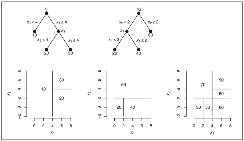
Suppose y_i represents the numeric outcome for individual i, and x_i is a vector of covariates with the regression relationship y_i = g(x_i; T, M) + e_i where i = 1, … , N. Notationally, g(x_i; T, M) is a binary tree function with components T and M that can be described as follows. T denotes the tree structure consisting of two sets of nodes: interior branches and terminal leaves. Each branch is a decision rule that is a binary split based on a single covariate. M = {μ₁, … , μ_b} is made up of the function values of the leaves. Each leaf is a numeric value: the value being the corresponding output of g when the branch rules applied to x_i uniquely determine the branch “climbing” route to a single leaf. Examples of two trees are shown in Figure 1 wherein branches appear as diamonds, and leaves as dots. Trees effectively partition the covariate space into rectangular regions, and these alternative representations are also shown in the figure.

Figure 1.

Two trees (left and center), and their sum (lower right only), fitted with two covariates, x1 and x2. Each tree is represented by branches (diamonds) and leaves (dots) as well as a rectangular partition of the covariate space.

BART employs an ensemble of such trees in an additive fashion, i.e. it is the sum of m trees where m is typically large such as 50, 100 or 200. Figure 1 shows a simple example of adding two trees. Note this sum of trees leads to a finer rectangular partition of the covariate space compared to each individual tree; here the value in each rectangular region is the sum of the leaves in each tree corresponding to that region. The model can be represented as

$$\phantom{\{}\begin{array}{c}{y}_i={\mu }_0+f({\mathit{x}}_i)+e_i\text{where}{e}_i\stackrel{\text{iid}}{\sim }\mathrm{N}(0,{\sigma }^2)\hfill \\ f({\mathit{x}}_i)=\sum _{j=1}^{m}g({\mathit{x}}_i;T_j,M_j)\hfill \end{array}\}$$ (1)

where μ₀ is typically set to $\overline{y}$. To proceed with the Bayesian paradigm, we need priors for the unknown parameters. We specify the prior for the error variance as ${\sigma }^2\stackrel{\text{prior}}{\sim }v\lambda {\chi }^2(v)$; details on specification of the parameters ν and λ are discussed in Chipman et al.¹⁸ And, notationally, we specify the prior for the unknown function, f, as

$$f\stackrel{\text{prior}}{\sim }\mathbf{BART}(m,{\mu }_0,\tau ,\alpha ,\gamma )$$ (2)

and describe it as made up of two components: a prior on the complexity of each tree, T_j, and a prior on its terminal nodes, M_j ∣T_j. Using the Smith-Gelfand generic bracket notation²⁰ as a shorthand for writing a probability density or conditional density, we write $[f]=\prod _j[T_j][M_j\mid T_j]$. Following Chipman et al.,¹⁸ we partition [T_j] into three components: the tree structure, or process by which we build a tree creating branches; the choice of a splitting covariate given a branch; and the choice of cut-point given the covariate for that branch. The probability of a node being a branch vs. a leaf is defined by describing the probabilistic process by which a tree is grown. We start with a tree that is just a single node, or root, and then randomly “grow” it into a branch (with two leaves) by the probability α(1 + d)^−γ where d represents the branch depth, α ∈ (0, 1) and γ ≥ 0. We assume that the choice of a splitting covariate given a branch, and the choice of a cut-point value given a covariate and a branch are both uniform. We then use the prior $[M_j\mid T_j]={\prod }_{\ell =1}^{b_j}[{\mu }_{j\ell }]$ where b_j is the number of leaves for tree j and ${\mu }_{j\ell }\stackrel{\text{prior}}{\sim }\mathrm{N}(0\frac{{\tau }^2}{m})$. Here $\tau =\frac{0.5}{\kappa }$ is parameterized in terms of a tuning parameter κ with default value of κ = 2 (as recommended in Chipman et al.¹⁸ and as used in the BART R package²¹). This gives f(x) ~ N(0, τ²) for any x since f(x) is the sum of m independent Normals. Along with centering of the outcome, these default prior parameters are specified such that each tree is a “weak learner” playing only a small part in the ensemble; more details on this can be found in Chipman et al.¹⁸

For data sets with a large number of covariates, P, Linero¹⁹ proposed replacing the uniform prior for selecting a covariate with a sparse prior. We refer to this alternative as the DART prior (the “D” is a mnemonic reference to the Dirichlet distribution). We represent the probability of variable selection via a sparse Dirichlet prior as $[s_1,\dots ,s_P]\stackrel{\text{prior}}{\sim }$ Dirichlet(θ/P, … , θ/P) rather than the uniform probability 1/P. The prior parameter θ can be fixed or random. Linero¹⁹ recommends that θ is random and specified via $\frac{\theta }{\theta +\rho }\stackrel{\text{prior}}{\sim }$ Beta(a, b) with the following sparse settings: ρ = P, a = 0.5 and b = 1. The distribution of θ, especially the parameters ρ and a, controls the degree of sparsity: a = 1 is not sparse while a = 0.5 is sparse and further sparsity can be achieved by setting ρ < P. This Dirichlet sparse prior helps the BART model naturally adapt to sparsity when P is large; both in terms of improving predictive performance as well as identifying important predictors in the model. Note that alternative variable selection methods exist for BART such as a permutation-based approach due to Bleich and Kapelner²² that is available in the bartMachine R package²³; however, we focus on the optional choice of incorporating the Dirichlet sparse prior into BART in subsequent competing risks models.

To apply the BART model to a binary outcome, we use a probit transformation

$$Pr(y=1\mid \mathit{x})\equiv p(\mathit{x})=\Phi ({\mu }_0+f(\mathit{x}))$$

where Φ is the standard normal cumulative distribution function and f ~ BART(m, μ₀, τ, α, γ). To estimate this model, we use the approach of Albert and Chib²⁴ and augment the model with latent variables z_i

$$\begin{gathered} y_i=I_{z_i\ge 0} \\ {z}_i={\mu }_0+f({\mathit{x}}_i)+e_i \\ f({\mathit{x}}_i)=\sum _{j=1}^{m}g({\mathit{x}}_i;T_j,M_j) \\ f\stackrel{\text{prior}}{\sim }\text{BART}(m,{\mu }_0,\tau ,\alpha ,\gamma ) \end{gathered}$$ (3)

where the indicator function I_z≥0 is one if z ≥ 0, zero otherwise; and $e_i\stackrel{\text{iid}}{\sim }N(0,1)$. The Albert and Chib method provides draws of f from the posterior via Gibbs sampling, i.e. draw z∣f, f ∣z, etc.

The model just described can be readily estimated using existing software for binary BART. It provides inference for the function f(x) through Markov Chain Monte Carlo (MCMC) draws of f from which the corresponding success probabilities, p(x) = Φ(μ₀ + f(x)), are readily obtained. Here μ₀ is typically set to ${\Phi }^{-1}(\overline{y})$. In the binary probit case, we let $\tau =\frac{3}{\kappa }$, so that there is 0.95 prior probability that f(x) is in the interval (−3, 3) giving a reasonable range of values for p(x). Note that Logistic latents, rather than Normal latents, could also be used for the binary outcome setting, and a Logistic implementation is also available in the BART package. However, because we are doing a prediction model and not focusing on parameter estimates like odds ratios, it is unclear whether probit or Logistic is more useful, so we have proceeded with the simpler and more computationally efficient probit framework.

Sparapani et al.¹³ adapted binary probit BART to the survival setting using discrete-time survival analysis.²⁵ We review this in detail, since a similar discrete-time approach is used here for the competing risks setting. Survival data are typically represented as (t_i, δ_i, x_i) where t_i is the event time, δ_i is an indicator distinguishing events (δ = 1) from right-censoring (δ = 0), x_i is a vector of covariates, and i = 1 , … , N indexes subjects. We denote the J distinct event and censoring times by 0 < t₍₁₎ < … < t_(J) < ∞ thus taking t_(j) to be the jth order statistic among distinct observation times and, for convenience, t₍₀₎ = 0. Now consider event indicators y_ij for each subject i at each distinct time t_(j) up to and including the subject’s observation time t_i = t_(ni) with n_i = #{j: t_(j) ≤ t_i} or n_i = arg max_j{t_(j) ≤ t_i}. This means y_ij = 0 if j < n_i and y_ini = δ_i. We then denote by p_ij probability of an event at time t_(j) conditional on no previous event. N.B. p_ij is the discrete hazard function. The likelihood has the form

$$L(p\mid \mathit{y})=\prod _{i=1}^N\prod _{j=1}^{n_i}{p}_{ij}^{y_{ij}}(1-p_{ij}{)}^{1-y_{ij}}$$ (4)

where the product over j is a result of the definition of p_ij’s as conditional probabilities, and not the consequence of an assumption of independence. Since this likelihood has the form of a binary likelihood for y_ij, we can apply the probit BART model where p_ij = Φ(μ₀ + f(t_(j), x_i)). Note the incorporation of t into the BART function f(t, x) allows the conditional probabilities to be time-varying, similar to a nonproportional hazards model.

With the data prepared as described above, the BART model for binary data treats the conditional probability of the event in an interval, given no events in preceding intervals, as a nonparametric function of the time t and the covariates x. Conditioned on the data, the algorithm in the BART package²¹ generates samples, each containing m trees, from the posterior distribution of f. For any t and x then, we can obtain posterior samples of

$$p(t,\mathit{x})=\Phi ({\mu }_0+f(t,\mathit{x}))$$

and the survival function

$$S(t_{(j)}\mid \mathit{x})=Pr(t>t_{(j)}\mid \mathit{x})=\prod _{l=1}^j(1-p(t_{(l)},\mathit{x})),j=1,\dots ,k$$

BART models with multiple covariates do not directly provide a summary of the marginal effect for a single covariate, or a subset of covariates, on the outcome. Marginal effect summaries are generally a challenge for nonparametric regression and/or black-box models. We use Friedman’s partial dependence function²⁶ with BART to summarize the marginal effect due to a subset of the covariates, x_S, by aggregating over the complement covariates, x_C, i.e., x = [x_S, x_C]. The marginal dependence function is defined by fixing x_S while aggregating over the observed settings of the complement covariates in the cohort as follows

$$f_S({\mathit{x}}_S)=N^{-1}\sum _{i=1}^{N}f({\mathit{x}}_S,{\mathit{x}}_{iC})$$ (5)

Consider the marginal survival function S_S(t∣x_S) = N⁻¹∑_iS(t∣x_S, x_iC). Other marginal functions can be obtained in a similar fashion. Marginal estimates can be derived via functions of the posterior samples such as means, quantiles, etc.

3. Competing risks and BART

Competing risks data are typically represented as (t_i, δ_i, ϵ_i, x_i) where ϵ_i ∈ {1, 2} denotes the event cause and, similar to before, t_i is the time to the event or censoring time, δ_i is an indicator distinguishing events (δ = 1) from right-censoring (δ = 0), x_i is a vector of covariates, and i = 1, … , N indexes subjects.

As before, we denote the J distinct event and censoring times by 0 < t₍₁₎ < … < t_(J) < ∞, and let n_i = arg max_j{t_(j) ≤ t_i}. The simplest way of representing the discrete time competing risks model is through a sequence of multinomial events y_ijk = I(t_i = t_(j), ϵ_i = k), i = 1, … , N; j = 1, … n_i; k = 1, 2 along with their corresponding conditional probabilities p_ijk = P(t_i = t_(j), ϵ_i = k∣t_i ≥ t_(j), x_i) that are interpreted as the probability of an event of cause k at time t_(j) given the patient is still at risk (has not yet experienced either cause of event) and given their covariates. Now, by successfully conditioning over time, we can write the likelihood as

$$L(p\mid \mathit{y})=\prod _{i=1}^N\prod _{j=1}^{n_i}{p}_{ij1}^{y_{ij1}}{p}_{ij2}^{y_{ij2}}(1-p_{ij1}-p_{ij2}{)}^{1-y_{ij1}-y_{ij2}}$$ (6)

Remark: the p_ijk are essentially a function of time, t, the patient’s covariates, x_i, and their interactions forming a general class of models which includes proportional cause-specific/subdistribution hazards models as special cases.

Since the likelihood matches that of a set of independent multinomial observations, one could directly apply BART models to the multinomial probabilities.²⁷ However, multinomial BART implementations are not as widely available, and their current approaches require estimation of the same number of BART functions as multinomial categories. We propose two alternative representations of the likelihood that facilitate direct use of the more prevalent binary probit BART implementations. Furthermore, our proposals are more computationally efficient by utilizing fewer BART functions to model the outcomes (two BART functions instead of three for a standard competing risk framework with two competing events).

Next, we present two methods, Method 1 and 2, for estimating this model. The model space for these two computational methods is the same. Yet, for any particular data set, this will lead to two different cumulative incidence function estimates. The differing estimates occur because the BART prior is applied to two different parameterizations of the model. However, since both models are flexible, we anticipate (and have observed) similar results.

3.1. Method 1

In this method, we rewrite the likelihood as

$$\begin{gathered} L(p\mid \mathit{y})=\prod _{i=1}^N\prod _{j=1}^{n_i}{\left(\frac{p_{ij1}}{p_{ij1}+p_{ij2}}\right)}^{y_{ij1}}{\left(\frac{p_{ij2}}{p_{ij1}+p_{ij2}}\right)}^{y_{ij2}}(p_{ij1}+p_{ij2}{)}^{y_{ij1}+y_{ij2}}(1-p_{ij1}-p_{ij2}{)}^{1-y_{ij1}-y_{ij2}} \\ =\prod _{i=1}^N\prod _{j=1}^{n_i}{p}_{ij.}^{y_{ij.}}(1-p_{ij.}{)}^{1-y_{ij.}}\prod _{i:{\delta }_i=1}{}_i^{u_i}(1-{\psi }_i{)}^{1-u_i} \end{gathered}$$ (7)

where p_ij· = p_ij1 + p_ij2, y_ij· = y_ij1 + y_ij2, u_i = I(ϵ_i = 1) and ψ_i = P(ϵ_i = 1∣t_i, δ_i = 1). This likelihood separates into two binary likelihoods, so that we can fit two separate BART probit models for p_ij· and ψ_i, using the corresponding binary observations y_ij· and u_i respectively. Specifically, we assume

$$\begin{gathered} y_{ij.}=I_{z_{ij}\ge 0} \\ {z}_{ij}={\mu }_y+f_y(t_{(j)},{\mathit{x}}_i)+e_{ij} \\ {f}_y\sim \text{BART}(m,{\mu }_y,\tau ,\alpha ,\gamma ) \end{gathered}$$ (8)

for the first model and

$$\begin{gathered} u_i=I_{{\tilde{z}}_i\ge 0} \\ {\tilde{z}}_i={\mu }_u+f_u(t_i,{\mathit{x}}_i)+{\tilde{e}}_i \\ {f}_u\sim \text{BART}(m,{\mu }_u,\tau ,\alpha ,\gamma ) \end{gathered}$$ (9)

for the second model. Conceptually, the first BART model is equivalent to a BART survival model for the time to the first event, while the latter BART model accounts for the probability of the event being of failure cause 1 given that an event occurs.

The algorithms in existing BART software provide for samples from the posterior distribution of f_y and f_u given the data. Similarly, samples from the posterior distribution of p_y(t, x) = Φ(μ_y + f_y(t, x)) and ψ(t, x) = Φ(μ_u + f_u(t, x)). Inference on the event-free survival distribution follows directly from p_y(t, x) as in Sparapani et al.¹³ using the expression

$$S(t_{(j)}\mid \mathit{x})=\prod _{l=1}^j(1-p_y(t_{(l)},\mathit{x})),j=1,\dots ,k$$

Inference on the cumulative incidence for cause 1 can be carried out using the expression

$$F_1(t_{(j)}\mid \mathit{x})=\sum _{l=1}^{j}S(t_{(l-1)}\mid \mathit{x})\psi (t_{(l)},\mathit{x})$$

With these functions in hand, one can easily accomplish inference for other quantities of interest based on the cumulative incidence function, such as conditional quantiles²⁸ defined as Q₁(τ∣x) = inf{t : F_k(t∣x ≥ τ)}. Analogous expressions for the cumulative incidence for the competing causes are also directly available. Note that Method 1 can easily be extended to multiple causes, i.e. cause 1 vs. cause 2 vs. cause 3, etc.

3.2. Method 2

In this method, we define ${\tilde{p}}_{ij2}=p_{ij2}∕(1-p_{ij1})$ as the conditional probability of event 2 at time t_(j) for patient i given that no cause 1 event occurred at that time, and re-express the likelihood as follows

$$\begin{gathered} L(p\mid \mathit{y})=\prod _{i=1}^N\prod _{j=1}^{n_i}{p}_{ij1}^{y_{ij1}}[{\tilde{p}}_{ij2}(1-p_{ij1}){]}^{y_{ij2}}(1-p_{ij1}-{\tilde{p}}_{ij2}(1-p_{ij1}){)}^{1-y_{ij1}-y_{ij2}} \\ =\prod _{i=1}^N\prod _{j=1}^{n_i}{p}_{ij1}^{y_{ij1}}(1-p_{ij1}{)}^{1-y_{ij1}}\prod _{i=1}^N\prod _{j:y_{ij1}=0}{\tilde{p}}_{ij2}^{y_{ij2}}(1-{\tilde{p}}_{ij2}{)}^{1-y_{ij2}} \end{gathered}$$ (10)

This likelihood also separates into two binary likelihoods, so that we can fit separate BART probit models for p_ij1 and ${\tilde{p}}_{ij2}$, using the corresponding binary observations y_ij1 and y_ij2 respectively. Specifically, we assume

$$\begin{gathered} y_{ij1}=I_{z_{ij1}\ge 0} \\ {z}_{ij1}={\mu }_1+f_1(t_{(j)},{\mathit{x}}_i)+e_{ij1} \\ {f}_1\sim \text{BART}(m,{\mu }_1,\tau ,\alpha ,\gamma ) \end{gathered}$$ (11)

for the first model and

$$\begin{gathered} y_{ij2}=I_{z_{ij2}\ge 0} \\ {z}_{ij2}={\mu }_2+f_2(t_{(j)},{\mathit{x}}_i)+e_{ij2} \\ {f}_2\sim \text{BART}(m,{\mu }_2,\tau ,\alpha ,\gamma ) \end{gathered}$$ (12)

for the second model. Conceptually, the first BART function models the conditional probability of a cause 1 event at time t_(j), given the patient is still at risk prior to time t_(j), while the second BART function models the conditional probability of a cause 2 event at time t_(j), given the patient is still at risk prior to time t_(j) and does not experience a cause 1 event. As above, the algorithms in existing BART software provide for samples from the posterior distribution of f₁ and f₂ given the data. Similarly, samples from the posterior distribution of p₁(t, x) = Φ(μ₁ + f₁(t, x)) and p₂(t, x) = Φ(μ₂ + f₂(t, x)) can be obtained. Samples from the event-free survival distribution are obtained from the expression

$$S(t_{(j)}\mid \mathit{x})=\prod _{l=1}^j(1-p_1(t_{(l)},\mathit{x}))(1-p_2(t_{(l)},\mathit{x})),j=1,\dots ,k$$

Samples from the cumulative incidence for cause 1 can be obtained using the expression

$$F_1(t_{(j)}\mid \mathit{x})=\sum _{l=1}^{j}S(t_{(l-1)}\mid \mathit{x})p_1(t_{(l)},\mathit{x})$$

3.3. Data construction

Competing risks data contained in observations (t, δ, ϵ) must be recast as binary outcome data; similarly, the corresponding time variable is recast as a covariate in order to fit the BART models described in both methods above.^29,30 For additional clarification, we give a very simple example of a data set with three observations here

$$(t_1,{\delta }_1,{\delta }_1{ϵ}_1)=(2.5,1,1),(t_2,{\delta }_2,{\delta }_2{ϵ}_2)=(1.5,1,2),(t_3,{\delta }_3,{\delta }_3{ϵ}_3)=(3,0,0)$$

where t₍₁₎ = 1.5, t₍₂₎ = 2.5, t₍₃₎ = 3.

For observation 1, the patient is at risk at time t₍₁₎ = 1.5, but does not experience an event, so that y₁₁₁ = 0, y₁₁₂ = 0, y_11· = 0. This same patient experiences a cause 1 event at time t₍₂₎ = 2.5, so that y₁₂₁ = 1 and y_12· = 1. However, because they experienced a cause 1 event at time t₍₂₎, the patient is no longer at risk of experiencing a cause 2 event using the Method 2 formulation of conditional probabilities, so we do not include y₁₂₂. For observation 1, u₁ = 1 since the patient experienced a cause 1 event at time t₁ = t₍₂₎. For observation 2, since the patient experiences a cause 2 event at time t₍₁₎ = 1.5, we define y₂₁₁ = 0, y₂₁₂ = 1, y_21· = 1, and u₂ = 0. For observation 3, since the patient is censored at t₍₃₎ = 3, all y_3jk = 0 for j = 1, … , 3 and k = 1, 2, · . Also, there is no u₃ defined for this patient since they did not experience any kind of event. A summary of the binary indicators and corresponding time covariates for each binary observation are summarized in Table 1. Besides time, the remaining covariates would contain the individual level covariates, x_i, with rows repeated to match the repetition pattern of the first subscript of y.

Table 1.

Data construction example.

i	j	t(j)	Method 1		Method 2
			yij.	ui	yij1	yij2
1	1	1.5	0		0	0
	2	2.5	1	1	1
2	1	1.5	1	0	0	1
3	1	1.5	0		0	0
	2	2.5	0		0	0
	3	3.0	0		0	0

By construction, the size of the data set is expanded from size N to roughly N² which can be problematic when N is large. This computational burden can be reduced by coarsening the time scale to K grid points where K << N, e.g. coarsening times in days to either weeks or months.

4. Performance of proposed methods

In order to determine the operating characteristics of our new method, we conducted several simulation studies and summarized various prediction performance metrics. We start with a two-sample setting to establish the face validity of the method to handle competing risks data with two groups. We then move on to examine performance in a complex regression setting.

4.1. Two sample setting

With a two-sample scenario, several settings are considered to represent standard modeling approaches to competing risks data: 1) proportional cause-specific hazards data generated from a Cox model; 2) proportional subdistribution hazards data generated from a Fine and Gray model; and 3) nonproportional subdistribution setting based on Weibull distributions. In each case, we simulate data sets with sample sizes of N = 250, 500, 1000 under independent exponential censoring with rate parameters leading to overall censoring proportions of 20% or 50%. Four different parameter settings are considered for each case. A total of 400 replicate data sets were generated in each instance.

4.1.1. Case 1: Proportional cause-specific hazards generated by the Cox model

For x ∈ {0, 1} and failure cause k ∈ {0, 1}, the cause specific hazard is given by λ_k(t, x) = λ_0ke^xβ_k where λ_0k > 0. The cumulative hazard for any cause of failure is given by Λ(t, x) = (λ₀₁e^xβ₁ + λ₀₂e^xβ₂)t, and the cumulative incidence for cause k is given by

$$F_k(t,x)=\frac{{\lambda }_k(t,x)}{{\lambda }_1(t,x)+{\lambda }_2(t,x)}[1-{\mathrm{e}}^{-\Lambda (t,x)}]$$

The limiting cumulative incidence for cause 1 in group x is

$$p_x=F_1(\infty ,x)=\frac{{\lambda }_{01}{\mathrm{e}}^{x{\beta }_1}}{{\lambda }_{01}{\mathrm{e}}^{x{\beta }_1}+{\lambda }_{02}{\mathrm{e}}^{x{\beta }_2}}$$

4.1.2. Case 2: Proportional subdistribution hazards generated by Fine and Gray’s model

Under a proportional subdistribution hazards model,³ the cumulative incidence functions can be directly specified as in Logan and Zhang³¹ as

$$F_1(t,x)=1-[1-p_0(1-{\mathrm{e}}^{-{\gamma }_{0}t}){]}^{{\mathrm{e}}^{x{\beta }_1}}$$ (13)

$$F_2(t,x)=(1-p_0{)}^{{\mathrm{e}}^{x{\beta }_1}}(1-{\mathrm{e}}^{-{\gamma }_{0}t})$$ (14)

4.1.3. Case 3: Nonproportional hazards based on Weibull subdistributions

To simulate this scenario, we describe a data generation process where first the failure cause is generated with probability p₀ for cause 1 regardless of group, and conditional on the failure cause, the failure time is generated from a Weibull distribution with scale parameter γ₀ and shape parameter e^xβ_k. Because the shape parameter is group dependent, this leads to different shapes of the cumulative incidence functions, with the same limiting cumulative incidence. The resulting cumulative incidence functions have the following form

$$F_k(t,x)=p_0^{2-k}(1-p_0{)}^{k-1}(1-e^{-{\gamma }_0{t}^{{}^{e^{x{\beta }_k}}}})$$

A summary of the parameter settings studied are in Table 2 below.

Table 2.

Parameter settings for Cases 1 through 3.

Case	λ01	λ02	β1	β2	p0	p1	γ0	γ1
1	1	1	0	0	0.5	0.5
Proportional	1	1	− log 2	log 2	0.5	0.2		2.5
Cox	2	0.5	0	0	0.8	0.8
	2	0.5	− log 2	log 2	0.8	0.5
2			0		0.5		2
Subdistribution			− log 2		0.5		2
Fine and Gray			0		0.8		2.5
			log 2		0.2		2.5
3			0	0	0.5		2
Nonproportional			− log 3	log 3	0.5		2
Weibull			0	0	0.8		2.5
			− log 3	log 3	0.2		2.5

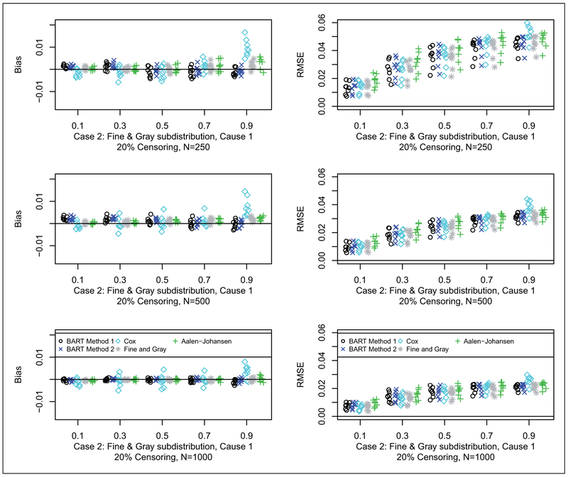
Each simulated data set was analyzed with both BART competing risks models, Cox proportional cause specific hazards models,³² Fine and Gray proportional subdistribution hazards model,³ and the Aalen-Johansen nonparametric estimator.³³ For brevity, we only consider cause 1 which is generally the cause of interest. For each scenario, we examined the prediction performance relative to the true cumulative incidence function in terms of bias and Root Mean Square Error (RMSE), at the following quantiles of the cdf: 10%, 30%, 50%, 70% and 90%. We also compare the 95% interval coverage probability and 95% interval length for the two BART methods. Results are plotted as points against quantile for each case and sample combination; note that there are 16 points (eight shown here and eight in the supplement) for each case and sample combination: two groups as targets for prediction, x = 0, 1; four parameter configurations, a = 1, 2, 3, 4 (shown in Table 2); and two censoring rates, 20% (shown here) and 50% (in the supplement), b = 0.2, 0.5. The bias and RMSE metrics were assessed at the five chosen quantiles, Q, of the event-free survival distribution, e.g. ${\text{bias}}_{Nxab}=H^{-1}{\sum }_h[{\widehat{F}}_{1,abh}(t_Q,x)-F_{1,ab}(t_Q,x)]$ where t_Q is such that Q = F_1,ab(t_Q, x) + F_2,ab(t_Q, x); N is the sample size; and h = 1, … , H are the simulated data sets. Similarly, the 95% interval coverage and length was assessed at the five chosen quantiles, e.g. ${\text{coverage}}_{Nxab}=H^{-1}{\sum }_h\mathrm{I}({\widehat{F}}_{1,abh,0.025}(t_Q,x)\le F_{1,ab}(t_Q,x)\le {\widehat{F}}_{1,abh,0.975}(t_Q,x))$.

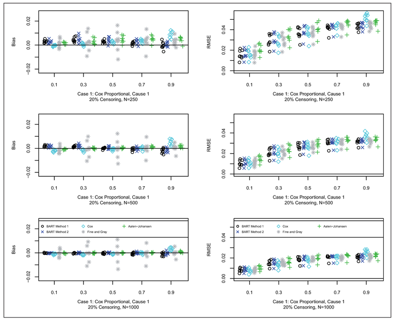
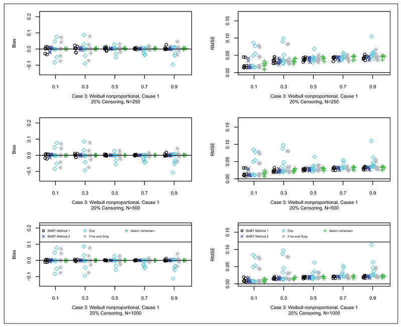
Results for bias and RMSE are shown for Cases 1, 2 and 3 in Figures 2 to 4, respectively (20% censoring shown here, 50% censoring in the supplement). In terms of bias, for Case 1, as anticipated, the Cox model approach generally has the smallest bias. For Case 2, as anticipated, the Fine and Gray method generally has the smallest bias. For Case 3, BART Method 2 generally has the smallest bias followed closely by BART Method 1. In terms of RMSE, for Case 1, generally all of the methods are quite competitive with respect to RMSE. Similarly for Case 2, all of the methods are quite competitive with respect to RMSE. For Case 3, the BART methods along with the Aalen-Johansen estimator generally have smaller RMSE than Cox and Fine and Gray. N.B. in the simulated data sets at the 90% time quantile with 50% censoring rate (coincidentally, approximately 90% quantile of the censoring distribution as well), on average there is only one data point at risk in a sample of size 250; whereas, for the 20% censoring rate, on average there are about 10 data points: therefore, at the 90% quantile with 50% censoring the errors are larger, particularly with BART, since it is so heavily data dependent due to data starvation.

Figure 2.

Bias (left) and RMSE (right) for case 1 with 20% censoring: N = 250 (first row), N = 500 (second row), and N = 1000 (third row). Each simulated data set was analyzed with both BART competing risks models, Cox proportional cause-specific hazards models, Fine and Gray proportional subdistribution hazards model, and the Aalen-Johansen nonparametric estimator. For brevity, we only consider cause 1 which is generally the cause of interest. For each scenario, we examined the prediction performance in terms of bias and Root Mean Square Error (RMSE), at the following quantiles of the cdf: 10%, 30%, 50%, 70% and 90%. Results are plotted as points against quantile for each case and sample combination; note that there are 16 points (eight shown here and eight in the supplement) for each case and sample combination: 2 groups as targets for prediction, x = 0, 1; 4 parameter configurations, a = 1, 2, 3, 4 (shown in Table 2); and 2 censoring rates, 20% (shown here) and 50% (in the supplement), b = 0.2, 0.5. The bias and RMSE metrics were assessed at the five chosen quantiles, Q, e.g. ${\text{bias}}_{Nxab}=H^{-1}{\sum }_h[{\widehat{F}}_{1,abh}(t_Q,x)-F_{1,ab}(t_Q,x)]$ where t_Q is such that Q = F_1,ab(t_Q, x) + F_2,ab(t_Q, x); N is the sample size; and h = 1, … , H are the simulated data sets.

Figure 4.

Bias (left) and RMSE (right) for case 3 with 20% censoring: N = 250 (first row), N = 500 (second row), and N = 1000 (third row). Each simulated data set was analyzed with both BART competing risks models, Cox proportional cause-specific hazards models, Fine and Gray proportional subdistribution hazards model, and the Aalen-Johansen nonparametric estimator. For brevity, we only consider cause 1 which is generally the cause of interest. For each scenario, we examined the prediction performance in terms of bias and Root Mean Square Error (RMSE), at the following quantiles of the cdf: 10%, 30%, 50%, 70% and 90%. Results are plotted as points against quantile for each case and sample combination; note that there are 16 points (eight shown here and eight in the supplement) for each case and sample combination: two groups as targets for prediction, x = 0, 1; four parameter configurations, a = 1, 2, 3, 4 (shown in Table 2); and wo censoring rates, 20% (shown here) and 50% (in the supplement), b = 0.2, 0.5. The bias and RMSE metrics were assessed at the five chosen quantiles, Q, e.g. ${\text{bias}}_{Nxab}=H^{-1}{\sum }_h[{\widehat{F}}_{1,abh}(t_Q,x)-F_{1,ab}(t_Q,x)]$ where t_Q is such that Q = F_1,ab(t_Q, x) + F_2,ab(t_Q, x); N is the sample size; and h = 1, … , H are the simulated data sets.

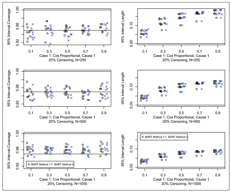
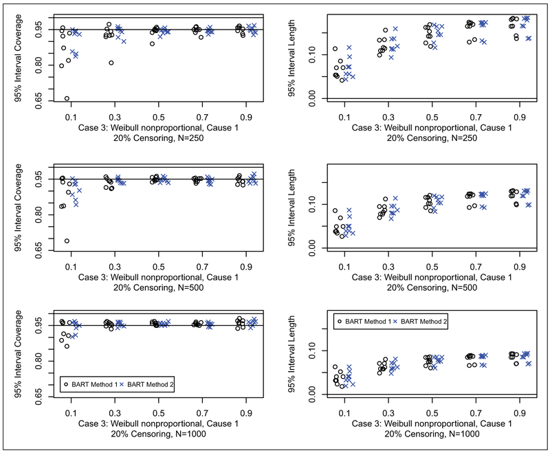
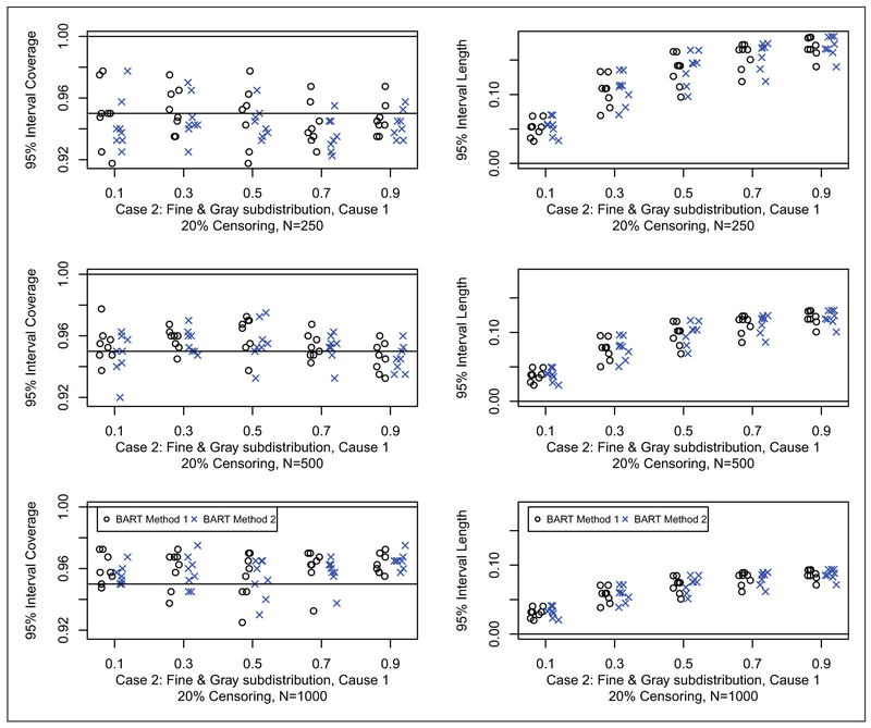
Results for coverage probabilities and interval length of 95% posterior intervals are shown for Cases 1, 2 and 3 in Figures 5 to 7, respectively (20% censoring shown here, 50% censoring in the supplement). For all cases, both of the BART methods have good coverage. There appears to be little difference in the width of the intervals between the two BART competing risk approaches. In summary, the BART methods perform comparable to the best method for each case considered in the two sample setting. This establishes the validity of the BART competing risks methodology as a flexible nonparametric estimator of the cumulative incidence function in the presence of a binary covariate. No noticeable differences in performance were seen between method 1 and method 2; however, method 1 has an advantage in terms of computation time because the second constructed data set used for the second BART function is substantially smaller (as can be clearly seen from u_i in Table 1).

Figure 5.

Coverage (left) and width (right) of 95% posterior intervals for case 1 with 20% censoring: N = 250 (first row), N = 500 (second row), and N = 1000 (third row). Each simulated data set was analyzed with both BART competing risks models. For brevity, we only consider cause 1 which is generally the cause of interest. For each scenario, we compare the 95% interval coverage probability and 95% interval length for the two BART methods. Results are plotted as points against quantile for each case and sample combination; note that there are 16 points (eight shown here and eight in the supplement) for each case and sample combination: two groups as targets for prediction, x = 0, 1; four parameter configurations, a = 1, 2, 3, 4 (shown in Table 2); and two censoring rates, 20% (shown here) and 50% (in the supplement), b = 0.2, 0.5. The 95% interval coverage and length was assessed at the five chosen quantiles, e.g. ${\text{coverage}}_{Nxab}=H^{-1}{\sum }_h\mathrm{I}({\widehat{F}}_{1,abh,0.025}(t_Q,x)\le F_{1,ab}(t_Q,x)\le {\widehat{F}}_{1,abh,0.975}(t_Q,x))$ where t_Q is such that Q = F_1,ab(t_Q, x) + F_2,ab(t_Q, x); N is the sample size; and h = 1, … , H are the simulated data sets.

Figure 7.

Coverage (left) and width (right) of 95% posterior intervals for case 3 with 20% censoring: N = 250 (first row), N = 500 (second row), and N = 1000 (third row). Each simulated data set was analyzed with both BART competing risks models. For brevity, we only consider cause 1 which is generally the cause of interest. For each scenario, we compare the 95% interval coverage probability and 95% interval length for the two BART methods. Results are plotted as points against quantile for each case and sample combination; note that there are 16 points (eight shown here and eight in the supplement) for each case and sample combination: two groups as targets for prediction, x = 0, 1; four parameter configurations, a = 1, 2, 3, 4 (shown in Table 2); and two censoring rates, 20% (shown here) and 50% (in the supplement), b = 0.2, 0.5. The 95% interval coverage and length was assessed at the five chosen quantiles, e.g. ${\text{coverage}}_{Nxab}=H^{-1}{\sum }_h\mathrm{I}({\widehat{F}}_{1,abh,0.025}(t_Q,x)\le F_{1,ab}(t_Q,x)\le {\widehat{F}}_{1,abh,0.975}(t_Q,x))$ where t_Q is such that Q = F_1,ab(t_Q, x) + F_2,ab(t_Q, x); N is the sample size; and h = 1, … , H are the simulated data sets.

4.2. Complex regression setting

While the above simulation establishes BART as a nonparametric estimator of the cumulative incidence function in the presence of a binary predictor, in practice, we are more interested in utilizing these approaches for modeling of competing risks data with more complex regression relationships. In this section, we demonstrate the performance of the proposed methods in a complex regression setting, and benchmark it against Random Survival Forests.^17,34 We generated two simulated data sets for each of the sample sizes; N = 500, 2000, 5000; for one data set we generated a small number of covariates, P = 10, and the other we generated a large number of covariates, P = 1000. This simulation study was carried out five times to ensure reproducibility. We base this setting on the Fine and Gray model³ since it provides a direct analytic expression for the cumulative incidence functions, and we only show the results of cause 1 for brevity. Because we are examining the impact of high dimensional predictors, we compare two variants of BART Method 1 against Random Survival Forests (RSF). The first variant is standard BART which chooses among the variables with a uniform prior. The second variant, which we call DART, substitutes a sparse Dirichlet prior for variable selection.

The basics of this setting are provided in Case 2 above. In the cumulative incidence expression (13), we set p₀ = 0.2 and γ₀ = 2.5, but replace xβ₁ with f(x) (which was inspired by Friedman’s five-dimensional test function³⁵): $f(\mathit{x})=0.5\sin (\pi x_1{x}_{(0.5P+1)})+x_2^2+0.5x_{(0.5P+2)}+0.25x_3^2-1.25$ where

$$x_j\sim \mathrm{U}(-1,1)j=1,\dots ,0.5P\text{and}{x}_{j^{\prime }}\sim \mathrm{U}(\{-1,1\})j^{\prime }=0.5P+1,\dots ,P$$

Note that this prescription provides f(x) ∈ [−1, 1].

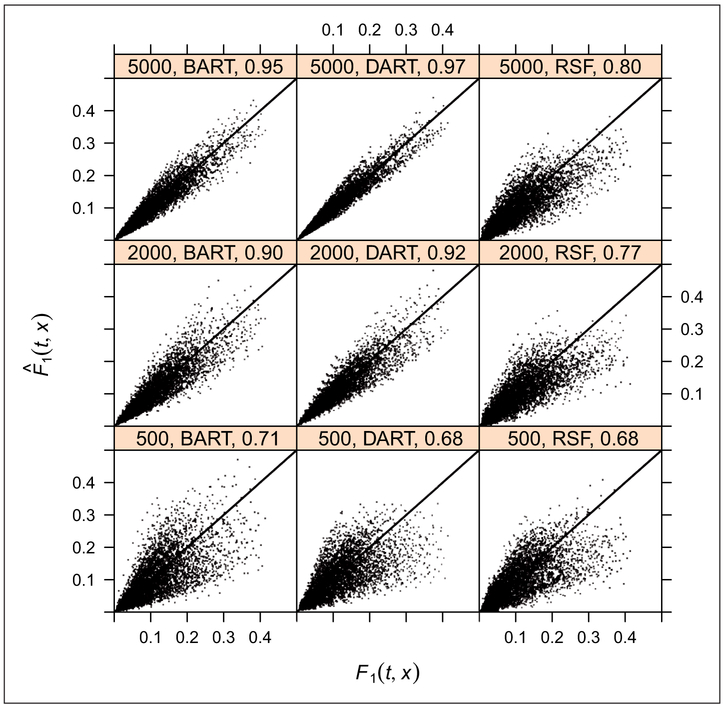
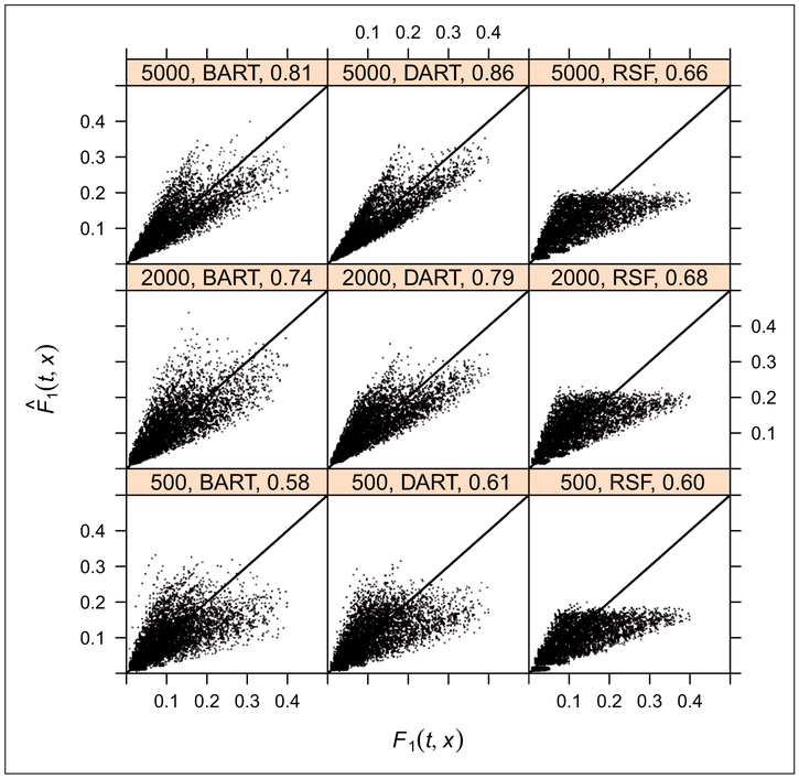
The models are fit to the randomly generated training data and applied to an independent test sample of size 500 in order to plot the predicted cumulative incidence against the known true CIF at the nine deciles of the uncensored true event times. We use Lin’s concordance coefficient, r_C(a, b) ∈ [−1, 1],³⁶ to assess prediction error: a correlation metric which penalizes departures from the diagonal, i.e. r_C(a, b) = +1 only when there is a direct linear relationship on the diagonal between the elements of the vectors a and b; similarly, r_C(a, b) = −1 only when there is an inverse linear relationship on the diagonal. Lin’s r_C is provided to summarize the agreement between the predicted, ${\widehat{F}}_1(t,\mathit{x})$, and true cumulative incidence function, F₁(t, x), for cause 1 at the nine deciles combined.

The results of the first simulation study for P = 10 and P = 1000 are shown in Figures 8 and 9, respectively (the other four simulation studies produced similar results). For P = 10, at N = 500, all three methods have roughly equivalent r_C around 0.7. When we get to N = 2000, DART has a slight advantage over BART and DART/BART have better performance than RSF. Similar results were obtained at N = 5000.

Figure 8.

Predicted vs. true F1(t, x) for BART, DART, and RSF, with P = 10, at sample sizes of N = 500, 2000, 5000. At N = 500, all three methods have roughly equivalent rC around 0.7. At N = 2000, 5000, DART has a slight advantage over BART and DART/BART have better performance than RSF. We demonstrate the performance of the proposed methods in a complex regression setting. We base this setting on the Fine and Gray model since it provides a direct analytic expression for the cumulative incidence functions, and we only show the results of cause 1 for brevity. Because we are examining the impact of high dimensional predictors, we compare two variants of BART Method 1 against Random Survival Forests (RSF). The first variant is standard BART which chooses among the variables with a uniform prior. The second variant, which we call DART, substitutes a sparse Dirichlet prior for variable selection. The basics of this setting are provided in Case 2 above, except that in the cumulative incidence expression (13), we set p₀ = 0.2 and γ₀ = 2.5, but replace xβ₁ with $f(x)=0.5\sin (\pi x_1{x}_{(0.5P+1)})+x_2^2+0.5x_{(0.5P+2)}+0.25x_3^2-1.25$ where x_j~U(−1, 1) j = 1, … , 0.5P and x_j′~U({−1, 1}) j^j = 0.5P + 1, … , P. The models are fit to the randomly generated training data and applied to an independent test sample of size 500 in order to plot the predicted cumulative incidence against the true CIF at the deciles of the uncensored true event times, t_Q. Lin’s concordance coefficient, r_C, is provided to summarize the agreement between the predicted, ${\widehat{F}}_1(t_Q,x)$, and true cumulative incidence function, F₁(t_Q, x), for cause 1.

Figure 9.

Predicted vs. true F1(t, x) for BART, DART, and RSF, with P = 1000, at sample sizes of N = 500, 2000, 5000. At N = 500, all three methods have roughly equivalent rC around 0.6. At N = 2000, 5000, DART has a slight advantage over BART and DART/BART have better performance than RSF. We demonstrate the performance of the proposed methods in a complex regression setting. We base this setting on the Fine and Gray model since it provides a direct analytic expression for the cumulative incidence functions, and we only show the results of cause 1 for brevity. Because we are examining the impact of high dimensional predictors, we compare two variants of BART Method 1 against Random Survival Forests (RSF). The first variant is standard BART which chooses among the variables with a uniform prior. The second variant, which we call DART, substitutes a sparse Dirichlet prior for variable selection. The basics of this setting are provided in Case 2 above, except that in the cumulative incidence expression (13), we set p₀ = 0.2 and γ₀ = 2.5, but replace xβ₁ with $f(x)=0.5\sin (\pi x_1{x}_{(0.5P+1)})+x_2^2+0.5x_{(0.5P+2)}+0.25x_3^2-1.25$ where x_j~U(−1, 1) j = 1, … , 0.5P and $x_j^{\prime }\sim \mathrm{U}(\{1,1\})j^j=0.5P+1,\dots ,P$. The models are fit to the randomly generated training data and applied to an independent test sample of size 500 in order to plot the predicted cumulative incidence against the true CIF at the deciles of the uncensored true event times, t_Q. Lin’s concordance coefficient, r_C, is provided to summarize the agreement between the predicted, ${\widehat{F}}_1(t_Q,x)$, and true cumulative incidence function, F₁(t_Q, x), for cause 1.

For P = 1000, at N = 500, all three methods have roughly equivalent r_C around 0.6. When we get to N = 2000, DART has a slight advantage over BART and DART/BART have better performance than RSF. Similar results were obtained at N = 5000. For RSF, surprisingly, all covariate combinations seem to converge on the same limiting cumulative incidence of roughly 0.2. This may be due to the inability of RSF to adapt to sparsity as reported by Linero¹⁹ without an explicit strategy for variable selection. Since only $\sqrt{P}$ variables are checked at each split, the likelihood of finding and splitting on important variables is low, leading to mostly random splits which would have a similar limiting cumulative incidence. We speculate that this could be mitigated by incorporating variable selection strategies based on variable importance measures directly into the algorithm.

5. Application to hematopoietic stem cell transplantation example

In this section, we apply the proposed BART competing risks method to a retrospective cohort study data set from the Center for International Blood and Marrow Transplant Research (CIBMTR) looking at the outcome of chronic graft-versus-host disease (cGVHD) after a reduced intensity hematopoietic cell transplant (HCT) from an unrelated donor³⁷ between the years 2000 and 2007. Development of cGVHD is the event of interest while death prior to development of cGVHD is the competing event. Patients with missing covariate data were removed to facilitate demonstration of the methods, so the results should be considered as an illustration of the methods rather than a clinical finding. A total of 427 cGVHD events and 324 competing risk events occurred in the 845 patients in the cohort. Thirteen covariates were considered in the analysis, including age, matched ABO blood type, year of transplant, disease/stage, matched human leukocyte antigens (HLA), graft type, Karnofsky Performance Score (KPS), cytomegalovirus (CMV) status of the recipient, conditioning regimen, use of in vivo T-cell depletion, graft-versus-host disease (GVHD) prophylaxis, matched donor-recipient sex and donor age, resulting in a total of 21 predictors in the X matrix. More details on the variables are available in Eapen et al.³⁷ The time scale was coarsened to weeks rather than days to reduce the computational burden.

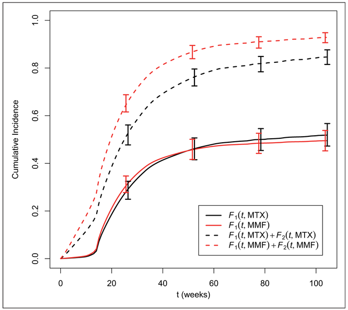
The BART competing risks Method 2 was fit to this data set with 200 trees, and the default settings for the rest of the prior settings, using a burn-in of 100 draws and thinning by a factor of 10, resulting in 2000 draws from the posterior distributions for the cumulative incidence function given covariates. Based on our simulation studies, we expect Method 1 to yield similar results, so we do not show it here. Partial dependence cumulative incidence functions can be obtained as in equation (5) for a particular subset of covariates. These can be interpreted as a marginal or average cumulative incidence function for that covariate level, averaged across the observed distribution of the remaining covariates. In the left panel of Figure 10, we show the stacked partial dependence cumulative incidence functions for each of two GVHD prophylaxis strategies, Methotrexate (MTX) based or Mycophenolate Mofitil (MMF) based. For each strategy, the CIF for cGVHD is shown as the bottom line, while the sum of the CIF for cGVHD and for death prior to cGVHD is shown as the upper line. These indicate that while there is very little difference in the incidence of cGVHD between these strategies overall, there seems to be a higher rate of death without cGVHD in the MMF group.

Figure 10.

Partial Dependence Stacked Cumulative Incidence Functions for two different GVHD prophylaxis strategies: MTX based or MMF based. Bottom line is the CIF for cGVHD, while top line represents the sum of the CIF for cGVHD and for the competing risk of death before cGVHD. 95% credible intervals provided at select time points.

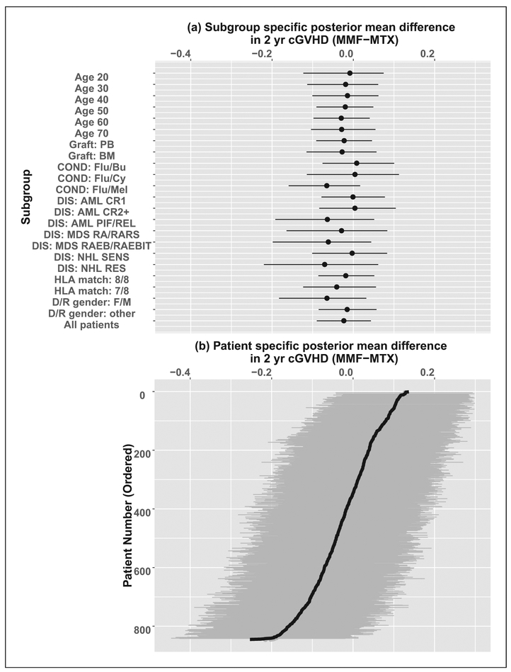
While there appears to be little difference in the CIF of cGVHD between the different GVHD prophylaxis strategies overall, it is also worth examining whether this is consistent across subgroups. We can use the partial dependence functions to examine the difference in CIF of cGVHD by two years between MTX and MMF in various subgroups. These are shown as a forest plot in Figure 11. These are generally consistent with the overall findings, with most subgroups showing posterior mean differences of less than 5% in the two-year CIF of cGVHD, and a few showing differences of up to 7%.

Figure 11.

Plots of the difference in two-year CIF for cGVHD, with 95% posterior interval, by (a) clinically defined subgroup, and (b) individual patient (ordered by mean difference). Subgroups are by age, graft type (PB = Peripheral Blood, BM = Bone Marrow), conditioning regimen (Flu = Fludarabine, Bu = Busulfan, Cy = Cyclophosphamide, Mel = Melphalan), disease/stage (AML = Acute Myelogenous Leukemia, MDS = Myelodysplastic Syndrome, NHL = Non-Hodgkin’s Lymphoma, CR = Complete Remission, PIF = Primary Induction Failure, REL = Relapse, RA = Refractory Anemia, RAR = RA with Ringed Sideroblasts, RAEB = RA with Excess Blasts, RAEBT = RAEB in Transmission), Human Leukocyte (HLA) matching between donor and recipient, and donor/recipient gender. Negative values indicate MMF has lower incidence of cGVHD.

The BART package can also be used to provide predictions of the difference in cumulative incidence between the GVHD prophylaxis regimens for each individual. These are shown in Figure 11(b), and show substantially more variability in the individual predictions compared to the subgroup mean predictions, as expected.

We examined the variable selection probabilities from fitting the DART model to this data set, to identify which variables have the highest posterior probabilities of being selected in the trees. Only five variables had at least a 5% mean posterior probability of being selected; these were, in order, time (48%), use of MMF as GVHD prophylaxis (7%), use of in vivo T-cell depletion (6%), use of Flu/Mel conditioning (6%), and AML patients in Primary Induction Failure or Relapse (6%). The first four of these were all selected in at least one of the trees in at least 90% of the posterior samples, while the last one was selected in 74% of the posterior samples. None of the other variables was selected as consistently in at least one of the trees.

We compared predictive performance of the proposed BART model to RSF on this BMT data using five-fold cross-validation estimates of Brier score and the C statistic from the pec R package.³⁸ C statistics at 1 and 2 years were 0.585 and 0.579 for BART and 0.589 and 0.583 for RSF, while Brier scores at 1 and 2 years were 0.240 and 225 for BART and 0.240 and 0.225 for RSF, indicating very similar predictive performance. Given the modest sample size and number of predictors, this result is consistent with the simulation results indicating similar performance of BART and RSF for smaller N and P, while the main advantage of BART was observed for larger N and P. Furthermore, BART directly provides measures of uncertainty which are not directly available from RSF.

6. Conclusion

In this article, we have proposed a novel approach for flexible modeling of competing risks data using BART. Our new methods have some strengths and weaknesses. We find the following strengths particularly compelling. The model handles a number of complexities in modeling, including nonlinear functions of covariates, interactions, high-dimensional parameter spaces, and nonproportional hazards (cause-specific or subdistribution). It has excellent prediction performance as a nonparametric ensemble prediction model.

Our formulation allows for the use of off-the-shelf BART software based on binary outcomes after restructuring the data as described. Furthermore, we have incorporated the competing risks BART models into our state-of-the-art BART R package²¹ which is publicly available on the Comprehensive R Archive Network (CRAN), https://cran.r-project.org, and distributed under the GNU General Public License.

BART can handle missing data which is often encountered in clinical research studies. For example, the BART package imputes one or more missing covariates by record-level hot-decking imputation³⁹ that is biased towards the null, i.e. non-missing values from another record are randomly selected regardless of the outcome. This simple missing data imputation method is sufficient for data sets with relatively few missing values. When necessary, more advanced missing data imputation approaches are available. The bartMachine R package²³ incorporates missing data indicators into the training data set allowing for splits on the missing indicators; this can improve performance under a pattern mixture model framework. An alternative approach uses sequential BART models to impute the missing covariates.^40,41

There are some weaknesses of our new approach that might not be immediately obvious. For example, these are complex models. While it is not straight forward to directly interpret the models themselves, any targets of inference, such as the overall survival or the cumulative incidence functions (as shown), are estimable including quantification of uncertainty. With a bit of additional effort, one can carry out inference for quantities such as cause-specific and subdistribution hazard ratios (not shown).

The methods proposed in this article can be computationally demanding, due to the need to expand the data at a grid of event times; although Method 1 is less demanding of the two. Nevertheless, we have found that the computation times are competitive with Random Survival Forests when you account for bootstrapping by RSF to obtain uncertainty estimates. For a large number of covariates, P, BART experiences only modest increases in computation time, while RSF suffers from substantial increases. Our approach can be parallelized, since the chains do not share information besides the data itself; simultaneously performing calculations on m chains can lead to substantial improvements in processing time (nearly linear for small m, but due to the burn-in penalty for each chain, diminishing returns as m increases further; see Amdahl’s law of parallel computing⁴²). Of course, there are other computational mitigation strategies like reducing the number of points in the time grid. By construction, the size of the data set is expanded from size N to roughly N² which can be problematic when N is large. This computational burden can be reduced by coarsening the time scale to K grid points where K << N, e.g. coarsening times in days to either weeks or months. We are currently investigating alternative models which do not require expansion of the data on a grid of event times.

Figure 3.

Bias (left) and RMSE (right) for case 2 with 20% censoring: N = 250 (first row), N = 500 (second row), and N = 1000 (third row). Each simulated data set was analyzed with both BART competing risks models, Cox proportional cause-specific hazards models, Fine and Gray proportional subdistribution hazards model, and the Aalen-Johansen nonparametric estimator. For brevity, we only consider cause 1 which is generally the cause of interest. For each scenario, we examined the prediction performance in terms of bias and Root Mean Square Error (RMSE), at the following quantiles of the cdf: 10%, 30%, 50%, 70% and 90%. Results are plotted as points against quantile for each case and sample combination; note that there are 16 points (eight shown here and eight in the supplement) for each case and sample combination: two groups as targets for prediction, x = 0, 1; four parameter configurations, a = 1, 2, 3, 4 (shown in Table 2); and two censoring rates, 20% (shown here) and 50% (in the supplement), b = 0.2, 0.5. The bias and RMSE metrics were assessed at the five chosen quantiles, Q, e.g. ${\text{bias}}_{Nxab}=H^{-1}{\sum }_h[{\widehat{F}}_{1,abh}(t_Q,x)-F_{1,ab}(t_Q,x)]$ where t_Q is such that Q = F_1,ab(t_Q, x) + F_2,ab(t_Q, x); N is the sample size; and h = 1, … , H are the simulated data sets.

Figure 6.

Coverage (left) and width (right) of 95% posterior intervals for case 2 with 20% censoring: N = 250 (first row), N = 500 (second row), and N = 1000 (third row). Each simulated data set was analyzed with both BART competing risks models. For brevity, we only consider cause 1 which is generally the cause of interest. For each scenario, we compare the 95% interval coverage probability and 95% interval length for the two BART methods. Results are plotted as points against quantile for each case and sample combination; note that there are 16 points (eight shown here and eight in the supplement) for each case and sample combination: two groups as targets for prediction, x = 0, 1; four parameter configurations, a = 1, 2, 3, 4 (shown in Table 2); and two censoring rates, 20% (shown here) and 50% (in the supplement), b = 0.2, 0.5. The 95% interval coverage and length was assessed at the five chosen quantiles, e.g. ${\text{coverage}}_{Nxab}=H^{-1}{\sum }_h\mathrm{I}({\widehat{F}}_{1,abh,0.025}(t_Q,x)\le F_{1,ab}(t_Q,x)\le {\widehat{F}}_{1,abh,0.975}(t_Q,x))$ where t_Q is such that Q = F_1,ab(t_Q, x) + F_2,ab(t_Q, x); N is the sample size; and h = 1, … , H are the simulated data sets.

References

- 1.Prentice RL, Kalbfleisch JD, Peterson A Jr, et al. The analysis of failure times in the presence of competing risks. Biometrics 1978; 34: 541–554. [PubMed] [Google Scholar]
- 2.Andersen PK, Borgan O, Gill RD, et al. Statistical models based on counting processes. New York, NY: Springer-Verlag, 1993, pp.512–515. [Google Scholar]
- 3.Fine JP and Gray RJ. A proportional hazards model for the subdistribution of a competing risk. J Am Stat Assoc 1999; 94: 496–509. [Google Scholar]
- 4.Klein JP and Andersen PK. Regression modeling of competing risks data based on pseudovalues of the cumulative incidence function. Biometrics 2005; 61: 223–229. [DOI] [PubMed] [Google Scholar]
- 5.Scheike TH, Zhang MJ and Gerds TA. Predicting cumulative incidence probability by direct binomial regression. Biometrika 2008; 95: 205–220. [Google Scholar]
- 6.Tibshirani R. The lasso method for variable selection in the Cox model. Stat Med 1997; 16: 385–395. [DOI] [PubMed] [Google Scholar]
- 7.Park MY and Hastie T. L1-regularization path algorithm for generalized linear models. J Royal Stat Soc: Ser B (Stat Methodol) 2007; 69: 659–677. [Google Scholar]
- 8.Zhang HH and Lu W. Adaptive lasso for Cox’s proportional hazards model. Biometrika 2007; 94: 691–703. [Google Scholar]
- 9.Ridgeway G. The state of boosting. Comput Sci Stat 1999; 31: 172–181. [Google Scholar]
- 10.Li H and Luan Y. Boosting proportional hazards models using smoothing splines, with applications to high-dimensional microarray data. Bioinformatics 2006; 21: 2403–2409. [DOI] [PubMed] [Google Scholar]
- 11.Ma S and Huang J. Clustering threshold gradient descent regularization: with applications to microarray studies. Bioinformatics 2006; 23: 466–472. [DOI] [PubMed] [Google Scholar]
- 12.Ishwaran H, Kogalur UB, Blackstone EH, et al. Random survival forests. Ann Appl Stat 2008; 2: 841–860. [Google Scholar]
- 13.Sparapani RA, Logan BR, McCulloch RE, et al. Nonparametric survival analysis using Bayesian Additive Regression Trees (BART). Stat Med 2016; 35: 2741–2753. [DOI] [PMC free article] [PubMed] [Google Scholar]
- 14.Van Belle V, Pelckmans K, Van Huffel S, et al. Improved performance on high-dimensional survival data by application of Survival-SVM. Bioinformatics 2010; 27: 87–94. [DOI] [PubMed] [Google Scholar]
- 15.Fu Z, Parikh CR and Zhou B. Penalized variable selection in competing risks regression. Lifetime Data Analys 2017; 23: 353–376. [DOI] [PubMed] [Google Scholar]
- 16.Ahn KW, Banerjee A, Sahr N, et al. Group and within-group variable selection for competing risks data. Lifetime Data Analys 2018; 24: 407–424. [DOI] [PMC free article] [PubMed] [Google Scholar]
- 17.Ishwaran H, Gerds TA, Kogalur UB, et al. Random survival forests for competing risks. Biostatistics 2014; 15: 757–773. [DOI] [PMC free article] [PubMed] [Google Scholar]
- 18.Chipman HA, George EI and McCulloch RE. BART: Bayesian additive regression trees. Ann Appl Stat 2010; 4: 266–298. [Google Scholar]
- 19.Linero A. Bayesian regression trees for high dimensional prediction and variable selection. J Am Stat Assoc 2018; 113: 626–636. [Google Scholar]
- 20.Gelfand AE and Smith AF. Sampling-based approaches to calculating marginal densities. J Am Stat Assoc 1990; 85: 398–409. [Google Scholar]
- 21.McCulloch R, Sparapani R, Gramacy R, et al. BART: Bayesian additive regression trees, https://cran.r-project.org/package=BART (accessed 24 December 2018). [Google Scholar]
- 22.Bleich J, Kapelner A, George EI, et al. Variable selection for BART: an application to gene regulation. Ann Appl Stat 2014; 8: 1750–1781. [Google Scholar]
- 23.Kapelner A and Bleich J. bartMachine: Bayesian additive regression trees, https://cran.r-project.org/package=bartMachine (2014). [Google Scholar]
- 24.Albert J and Chib S. Bayesian analysis of binary and polychotomous response data. J Am Stat Assoc 1993; 88: 669–679. [Google Scholar]
- 25.Fahrmeir L. Discrete survival-time models In: Armitage P and Colton T (eds) Encyclopedia of biostatistics. Chichester: Wiley, 1998, pp.1163–1168. [Google Scholar]
- 26.Friedman JH. Greedy function approximation: a gradient boosting machine. Ann Stat 2001; 29: 1189–1232. [Google Scholar]
- 27.Murray JS. Log-linear Bayesian additive regression trees for categorical and count responses. arXiv preprint 2017; arXiv: 1701.01503. [Google Scholar]
- 28.Peng L and Fine JP. Competing risks quantile regression. J Am Stat Assoc 2009; 104: 1440–1453. [Google Scholar]
- 29.Singer JD and Willett JB. It’s about time: Using discrete-time survival analysis to study duration and the timing of events. J Educ Stat 1993; 18: 155–195. [Google Scholar]
- 30.Allison PD. Survival analysis using the SAS system: a practical guide. Cary, NC: SAS Institute Inc, 1995. [Google Scholar]
- 31.Logan BR and Zhang MJ. The use of group sequential designs with common competing risks tests. Stat Med 2013; 32: 899–913. [DOI] [PMC free article] [PubMed] [Google Scholar]
- 32.Cox DR. Regression models and life-tables (with discussions). Jr Stat Soc B 1972; 34: 187–220. [Google Scholar]
- 33.Aalen OO and Johansen S. An empirical transition matrix for non-homogeneous Markov chains based on censored observations. Scand J Stat 1978; 5: 141–150. [Google Scholar]
- 34.Ishwaran H and Kogalur UB. Random forests for survival, regression and classification (RF-SRC), https://CRAN.R-project.org/package=randomForestSRC (2018). [Google Scholar]
- 35.Friedman JH. Multivariate adaptive regression splines. Ann Stat 1991; 19: 1–67. [DOI] [PubMed] [Google Scholar]
- 36.Lawrence I and Lin K. A concordance correlation coefficient to evaluate reproducibility. Biometrics 1989; 45: 255–268. [PubMed] [Google Scholar]
- 37.Eapen M, Logan BR, Horowitz MM, et al. Bone marrow or peripheral blood for reduced-intensity conditioning unrelated donor transplantation. J Clin Oncol 2015; 33: 364–369. [DOI] [PMC free article] [PubMed] [Google Scholar]
- 38.Gerds T. pec: Prediction error curves for risk prediction models in survival analysis, https://cran.r-project.org/package=pec (2018). [Google Scholar]
- 39.de Waal T, Pannekoek J and Scholtus S. Handbook of statistical data editing and imputation. Hoboken, NJ: John Wiley & Sons, 2011. [Google Scholar]
- 40.Xu D, Daniels MJ and Winterstein AG. Sequential BART for imputation of missing covariates. Biostatistics 2016; 17: 589–602. [DOI] [PMC free article] [PubMed] [Google Scholar]
- 41.Daniels M and Singh A. sbart: Sequential BART for imputation of missing covariates, https://CRAN.R-project.org/package=sbart (2018). [DOI] [PMC free article] [PubMed] [Google Scholar]
- 42.Amdahl G. Validity of the single processor approach to achieving large-scale computing capabilities. In: AFIPS conference proceedings Atlantic City, NJ, USA, 18–20 April 1967, pp.483–485. [Google Scholar]
Associated Data
This section collects any data citations, data availability statements, or supplementary materials included in this article.